Magnetic flux induce dissipation effect on the quantum phase diagram of mesoscopic SQUID array

Abstract

We present the quantum phase diagram of mesoscopic SQUID array. We predict different quantum phases and the phase boundaries along with several special points. We present the results of magnetic flux induced dissipation on these points and also on the phase boundaries. The Josephson couplings at these points are dependant on the system parameter in a more complicated fashion and differ from the Ambegaokar and Baratoff relation. We derive the analytical relation between the dissipation strength and Luttinger liquid parameter of the system. We observe some interesting behaviour at the half-integer magnetic flux quantum and also the importance of co-tunneling effect.

Keywords: Mesoscopic and nanoscale system, Josephson junction arrays and wire networks, SQUID devices
PACS: 74.78.Na, 74.81.Fa, 82.25.Dq.

I 1. Introduction

Josephson junction arrays have attracted considerable interest in the recent years owing to their interesting physical properties like quantum phase transition, quantum critical behaviour and Coulomb blockade etc schon ; fazio . The most universally observed behaviour for the low-dimensional superconducting system is the superconductor-insulator transition in superconducting flim, wires, Josephson junction array in one and two dimensional giving rise to intense experimental and theoretical activity havi1 ; mason ; bezr ; bezr2 ; sondhi ; lar ; suj1 ; suj2 ; geer ; zant ; havi3 ; kuo ; gran ; chen ; refa This superconductor-insulator transition occurs at low temperature ( mili-Kelvin scale) due the variation of one of the parameter of the system such as the normal state resistance of the flim, thickness of the wire, the Josephson coupling of Josephson junction array and the magnetic flux of the mesoscopic SQUID array.
In one dimensional superconducting quantum dot lattice system (mesoscopic SQUID array, Cooperpair box array) one elementary excitation occurs, i.e., the quantum phase slip centers (QPS) suj2 ; kuo ; chen ; refa . Recently the physics of QPS and the related physics has been studied extensively. Quantum phase slip process is a topological excitation, it’s a discrete process in space-time domain of a one dimensional superconducting system. In this process the amplitude of the order parameter destroys temporarily at a particular point that leads the phase of the order parameters to change abruptly (in units of 2 $\pi$). This process occurs at the time of macroscopic quantum tunneling of the system. As we understand from our previous study suj2 and also from the existing literature that the QPS process initiate the superconductor- insulator transition chen ; refa . It is well known after the work of Calderia and Leggett cal the dissipation plays a central role in the macroscopic quantum system. There are several study in the literature based on the Calderia-Leggett formalism to explain the different physical properties of low-dimensional tunneling junction system sch1 ; su1 ; su2 ; schon2 ; kane ; furu ; zai1 . We are mainly motivated from the experimental findings of Chow $et~{}al$ havi3 . They have done some pioneering work to study the effect of magnetic flux on mesoscopic SQUIDs array. They have observed the magnetic flux induced dissipation driven superconductor-insulator quantum phase transition and the evidence of qunatum critical point. The other interesting part of this study the length scale dependent superconductor-insulator transition and the magnertic flux induced superconductivity.
The goal of this paper is to provide a detailed analysis of the appearance of different quantum phases and phase boundaries in the presence and absence of dissipation for a mesoscopic SQUID array at $T=0$. We assume the presence of ohomic dissipation motivated by the experiment in Ref. (havi3 ) and we study the consequence of it in the different quantum phases and phase boundaries and also on the special points like the particle-hole symmetric point, charge degeneracy point, and multicritical points. We also derive the relation between the dissipation strength and Luttinger liquid parameter of the system. We are able to find out the relation between the Josephson coupling and the other interaction parameters of the system through the analysis of Luttinger liquid parameter of the system , we will notice that this analytical relation is more complicated and differs from the Ambegaokar-Baratoff ambe relation. To the best of our knowledge, this is the first derivation in the literature. The plan of the manuscript is as follows. In section 2A, we introduce the basic concept of the appearence of quantum phase slip centers and the source of dissipation for one dimensional superconducting quantum dot lattice. In section 2B, we derive the relation between the dissipation strength and the Luttinger liquid parameter of the system. In section 3, We present the analysis of quantum phases and phase boundaries, in the presence and absence of magnetic flux induced dissipation. Section IV, is devoted for summary and conclusions.

Figure 1: A. Schematic diagram of one dimensional array of small capacitance dc SQUIDs. Each plaque is a SQUID with two Josephson junctions marked by the cross. Circle with plus sign represent the applied magnetic flux $\Phi$. B. Equivalent representation of system A, where the dots are connected through tunnel junctions and the Josephson couplings of this system is tunable due to presence of magnetic flux $\Phi$.

II 2. Basic Aspects of Quantum Phase Slip Centers and Analytical Derivations of Dissipative Strengths in Terms of Luttinger liquid parameter

II.1 2A. Basic Aspects of Quantum Phase Slip Centers:

It is well known to us that the Josephson coupling of the SQUID is modulated by a facror, $E_{J1}=E_{J}|cos(\frac{\pi{\phi}}{{\phi}_{0}})|$, where $\phi$ is the magnetic flux and ${\phi}_{0}=\frac{hc}{2e}$ is the magnetic flux quantum. Therefore we can consider the the mesoscopic SQUIDs array as a superconducting quantum dot (SQD) lattice with modulated Josephson junction suj1 ; suj2 . Fig. 1 shows the equivalance between the mesoscopic SQUIDs array and SQD lattice with modulated Josephson junctions. Here we prove the appearance of QPS in SQD array with modulated Josephson coupling through an analysis of a minimal model. We consider two SQDs are separated by a Josephson junction. These two SQDs are any arbitrary SQDs of the array. Appearance of QPS is an intrinsic phenomenon (at any junction at any instant) of the system. The Hamiltonian of the system is

$$H~{}=~{}\sum_{i}~{}\frac{{n_{i}}^{2}}{2C}~{}-~{}{E_{J}}|cos(\frac{\pi\Phi}{{\Phi}_{0}})|\sum_{i}cos(~{}{\theta}_{i+1}~{}-~{}{\theta}_{i})$$ (1)

where $n_{i}$ and ${\theta}_{i}$ are respectively the Cooper pair density and the superconducting phase of the i’th dot and $C$ is the capacitance of the junction. The first term of the Hamiltonian present the Coulomb charging energies between the dots and the second term is nothing but the Josephson phase only term with modulated coupling, due to the presence of magnetic flux. We will see that this model is sufficient to capture the appearance of QPS in SQD systems. Hence this Hamiltonian has sufficient merit to capture the low temperature dissipation physics of SQD array. In the continuum limit, the partition function of the system is given by, $Z=\int D\theta(x,\tau)~{}e^{-~{}{S_{Q}}(x,\tau)},$ where $S_{Q}=\int d\tau\int dx\frac{E_{J}}{2}~{}[{({\partial}_{\tau}\theta(x,\tau))}^{2}+{({\partial}_{x}\theta(x,\tau))}^{2}]$. This action is quadratic in scalar-field $\theta(x,\tau)$, where $\theta(x,\tau)$ is a steady and differentiable field, so one may think that no phase transition can occur for this case. This situation changes drastically in the presence of topological excitations for which $\theta(x,\tau)$ is singular at the center of the topological excitations. So for this type of system, we express the $\theta(x,\tau)$ into two components: $\theta(x,\tau)={{\theta}_{0}}(x,\tau)+{{\theta}_{1}}(x,\tau)$, where ${{\theta}_{0}}(x,\tau)$ is the contribution from attractive interaction of the system and ${{\theta}_{1}}(x,\tau)$ is the singular part from topological excitations. We consider at any arbitrary time $\tau$, a topological excitation with center at $X(\tau)~{}=~{}({x_{0}}(\tau),{{\tau}_{0}}(\tau))$ . The angle is measured from the center of topological excitations between the spatial coordinate and the x-axis ${{\theta}_{1}}(x,\tau)~{}=~{}tan^{-1}(~{}\frac{{\tau}_{0}-\tau}{x_{0}-x})$ . The derivative of the angle is ${\nabla}_{x}{{\theta}_{1}}(x-X(\tau))~{}=~{}\frac{1}{{|x-X(\tau)|}^{2}}[-({\tau}_{0}-\tau),(x-x_{0})]$ which has a singularity at the center of the topological excitation. Finally we get an interesting result when we integrate along an arbitrary curve encircling the topological excitations. $\int_{C1}dx{\nabla}_{x}{{\theta}_{1}}(x-X(\tau))~{}=~{}2\pi.$ So we conclude from our analysis that when a topological excitation is present in the SQD array, the phase difference ,$\theta$, across the junction of quantum dots jumps by an integer multiple of $2\pi$. This topological excitation is nothing but the QPS in the $(x,\tau)$ plane. According to the phase voltage Josephson relation , $V_{J}~{}=~{}\frac{-1}{2e}\frac{d\theta}{dt}$ ($t$ is the time), a voltage drop occurs during this phase slip, which is the source of dissipation.

II.2 2B. Analytical Derivations of Dissipative Strengths in Terms of Luttinger Liquid Parameters

Here we derive analytical expression of magnetic flux induced dissipative strength (${\alpha}$) in terms of the interactions of the system. At first we derive the dissipative action/partition function of a quantum impurity system. In our study, we consider the backscattering process from a quantum impurity to compare the effective action with the superconducting tunnel junction system. We will see that the analytical structure of this dissipative action is identical with the mesoscopic SQUIDs array. In a different context, the authors of Ref. caza have predicted the dissipation driven quantum phase transition to occur. They have also considered the presence of backscattering events originated in the LL under the effect of dynamically screened Coulomb interaction.
Here we consider that the impurity is present at the origin where the fermions scatter from the left to the right and vice versa. The Hamiltonian describing this process is

$${H_{1}}={V_{0}}({R^{\dagger}}(0){L}(0)+h.c)={V_{0}}\int dx{\delta}(x)cos{\theta}(x).$$

The total Hamiltonian of the system is

$$H={H_{0}}~{}+~{}{V_{0}}\int dx{\delta}(x)cos{\theta}(x,\tau)$$ (2)

$${H_{0}}=\frac{1}{2\pi}\int{uK{({{\partial}_{x}}{\theta}(x,\tau))}^{2}~{}+~{}\frac{u}{K}{({{\partial}_{x}}{\phi}(x,\tau))}^{2}},$$ (3)

The corresponding Lagrangian of the system is

$${L} = \frac{1}{2\pi K}\int{\frac{1}{u}{({{\partial}_{\tau}}{\phi}(x,\tau))}^{2}~{}+~{}{u}{({\partial}{\phi}(x,\tau))}^{2}}$$ (4)

$$+{V_{0}}\int dx\delta(x)cos(\theta(x,\tau))={L_{0}}+{L_{1}}$$

where ${L_{0}}$ and ${L_{1}}$ are the non-interacting and the interacting part of the Lagrangian and $K$ is the Luttinger liquid parameter of the system. The only non-linear term in this Lagrangian is expressed by the field $\theta(x=0)$. We would like to express the action of the system as an effective action by integrating the field $\theta(x\neq 0)$. Therefore one may consider $\theta(x\neq 0)$ as a heat bath, which yields the source of dissipation in the system. The constraint condition for the integration is ${\theta}(\tau)={\theta}(x=0,\tau)$. We can write the partition function of the quantum impurity system. $Z=\int D\theta(x,\tau)D\theta(\tau)\delta(\theta(\tau)-{\theta}(0,\tau))e^{-\int_{0}^{\beta}Ld{\tau}}$ Now we use the standard trick of introducing the Lagrange multiplier with auxiliary field $\lambda(\tau)$.

$$Z = \int{D\theta(\tau)}e^{-\int_{0}^{\beta}{L_{1}}d{\tau}}\int D{\lambda(\tau)}e^{-i{\lambda(\tau)}{\theta}(\tau)}$$ (5)

$$\int{D\theta(x,\tau)}e^{\int_{0}^{\beta}(-{L_{0}}+i{\lambda}({\tau}){\theta}(0,\tau)){d\tau}}$$

The Fourier transform of the first term of Eq.(3) is ${L_{0}}~{}=~{}\sum_{q}\sum_{i{\omega}_{n}}\frac{{{\omega}_{n}}^{2}~{}+~{}{v}^{2}{q}^{2}}{2\pi Kv}{\theta}(q,i{{\omega}_{n}}){\theta}(-q,-i{{\omega}_{n}})$. At first we would like to calculate the integral: $\int_{0}^{\beta}d{\tau}[{L_{0}}-i{\lambda(\tau)}{\theta(0,\tau)}]$, we can write this term as

$$\sum_{q}\sum_{i{\omega}_{n}}\frac{{{\omega}_{n}}^{2}~{}+~{}{v}^{2}{q}^{2}}{2\pi Kv}{\theta}(q,i{{\omega}_{n}}){\theta}(-q,-i{{\omega}_{n}})$$

$$-\frac{1}{2\sqrt{L}}({\lambda}(i{\omega}_{n}){\theta}(-q,-i{{\omega}_{n}})+{\lambda}(-i{\omega}_{n}){\theta}(q,i{{\omega}_{n}}).$$ (6)

This integral appears in the integral $\theta(x,\tau)$. This integral is quadratic in $\theta$. Now we would like to perform the Gaussian integration by completing the square. We can write the result as $\frac{-1}{2L}\sum_{i{{\omega}_{n}},q}\frac{\pi Kv}{{{\omega}_{n}}^{2}~{}+~{}{v}^{2}{q}^{2}}$. In the infinite length limit one can write,
$\frac{1}{2L}\sum_{q}\frac{\pi Kv}{{{\omega}_{n}}^{2}~{}+~{}{v}^{2}{q}^{2}}~{}=~{}\int\frac{dq}{2\pi}\frac{\pi Kv}{{{\omega}_{n}}^{2}~{}+~{}{v}^{2}{q}^{2}}=\frac{\pi K}{4{{\omega}_{n}}}$.
Now we would like to append this result of integration in the second integral of $Z$, i.e., the integral over ${\lambda}$. One can write the integrand as

$$\sum_{i{{\omega}_{n}}}(-\frac{\pi K}{4{{\omega}_{n}}}{\lambda}(i{\omega}_{n}){\lambda}(-i{\omega}_{n})+\frac{i}{2}({\lambda}(i{\omega}_{n}){\theta}(-q,-i{{\omega}_{n}})$$

$$+{\lambda}(-i{\omega}_{n}){\theta}(q,i{{\omega}_{n}}).$$ (7)

This integral is again the quadratic integral of $\lambda$, therefore, the Gaussian integral can be performed by completing the square. We perform the integration and finally obtain $\sum_{i{{\omega}_{n}}}\frac{{\omega}_{n}}{\pi K}\theta(i{\omega}_{n})\theta(-i{\omega}_{n})$. From this analytical expression, we obtain the effect of bath on ${\theta}(\tau)$. Appearance of the factor ${{\omega}_{n}}$ signifies the dissipation. Therefore, the effective action reduces to

$$S~{}=~{}\sum_{i{{\omega}_{n}}}\frac{{\omega}_{n}}{\pi K}\theta(i{\omega}_{n})\theta(-i{\omega}_{n})+\int d{\tau}{V_{0}}cos{\theta}(\tau)$$ (8)

The above action implies that a single particle moves in the potential ${V_{0}}cos{\theta}(\tau)$ subject to dissipation with friction constant , $\frac{1}{\pi K}$.

Now we calculate the dissipative action of mesoscopic SQUIDs array. Here, we calculate the effective partition function of our system. Our starting point is the Calderia-Legget cal formalism. Following this reference we write the action as

$$S_{1}~{}=~{}S_{0}~{}+~{}\frac{{\alpha}}{4\pi T}~{}\sum_{m}{{\omega}_{m}}{|{\theta}_{m}|}^{2}.$$ (9)

$S_{0}$ is the action for non-dissipative part and $S_{1}$ is the standard action for the system with tilted wash-board potential sch1 ; su1 ; schon to describe the dissipative physics for low dimensional superconducting tunnel junctions, ${\alpha}$ is the dissipative strength of the system,

$${\alpha}~{}=~{}\frac{R_{Q}}{R_{s}}cos|\frac{\pi\phi}{{\phi}_{0}}|$$ (10)

(the extra cosine factor which we consider in ${\alpha}$ is entirely new which probes the effect of an external magnetic flux and is also consistent physically), ${\omega}_{m}~{}=~{}\frac{2\pi}{\beta}m$ is the Matsubara frequency and $R_{Q}$ ($=6.45k\Omega$) is the quantum resistance, $R_{s}$ is the tunnel junction resistance, $\beta$ is the inverse temperature. In one of our previous work, we have explained few experimental findings by using the above expression of ${\alpha}$. In the strong potential, tunneling between the minima of the potential is very small. In the imaginary time path integral formalism, tunneling effect in the strong coupling limit can be described in terms of instanton physics. In this formalism, it is convenient to characterize the profile of $\theta$ in terms of its time derivative,

$$\frac{d\theta{(\tau)}}{d{\tau}}~{}=~{}\sum_{i}e_{i}h(\tau-{\tau}_{i}),$$ (11)

where $h(\tau-{\tau}_{i})$ is the time derivative at time $\tau$ of one instanton configuration. ${\tau}_{i}$ is the location of the i-th instanton, $e_{i}=1$ and $-1$ is the topological charge of instanton and anti-instanton respectively. Integrating the function over $h$ from $-\infty$ to $\infty$, we get $\int_{-\infty}^{\infty}d\tau h(\tau)={\theta}(\infty)-{\theta}({-\infty})=2\pi.$ It is well known that the instanton (anti-instanton) is almost universally constant except for a very small region of time variation. In the QPS process the amplitude of the superconducting order parameter is zero only in a very small region of space as a function of time and the phase changes by $\pm 2\pi$. So our system reduces to a neutral system consisting of equal number of instanton and anti-instanton. One can find the expression for ${\theta}(\omega)$ after the Fourier transform applied to both the sides of Eq. 11 which yields ${\theta}(\omega)=\frac{i}{\omega}\sum_{i}e_{i}h(i\omega)e^{i{\omega}{\tau}_{1}}$ . Now we substitute this expression for ${\theta}(\omega)$ in the second term of Eq. 9 and finally we get this term as $\sum_{ij}~{}F({\tau}_{i}-{\tau}_{j}){e_{i}}{e_{j}}$, where $F({\tau}_{i}-{\tau}_{j})=\frac{\pi\alpha}{\beta}\sum_{m}~{}\frac{1}{{|{\omega}_{m}}|}e^{i{\omega}({\tau}_{i}-{\tau}_{j})}$ $\simeq ln({\tau}_{i}-{\tau}_{j})$. We obtain this expression for very small values of ${\omega}$ ( $\rightarrow 0$). So $F({\tau}_{i}-{\tau}_{j})$ effectively represents the Coulomb interaction between the instanton and anti-instanton. This term is the main source of dissipation of SQUID array system. Following the standard prescription of imaginary time path integral formalism, we can write the partition function of the system as suj2 ; lar ; gia1 ; kane ; zai1 ; furu .

$$Z = \sum_{n=0}^{\infty}\frac{1}{n!}{z}^{n}\sum_{e_{i}}\int_{0}^{\beta}d{{\tau}_{n}}\int_{0}^{{\tau}_{n-1}}d{\tau}_{n-1}...$$ (12)

$$\int_{0}^{{\tau}_{2}}d{{\tau}_{1}}e^{-F({\tau}_{i}-{\tau}_{j}){e_{i}}{e_{j}}}.$$

We would like to express the partition function in terms of integration over auxiliary field, $q{(\tau)}$. After some extensive analytical calculations, we get

$$Z=\int Dq(\tau)e^{(-\sum_{i{\omega}_{n}}\frac{|{{\omega}_{n}}|}{4\pi{\alpha}}q(i{\omega}_{n})q(-i{\omega}_{n})){+(2z\int_{0}^{\beta}d{\tau}cosq(\tau))}}.$$ (13)

Thus by comparing the first term of the action of Eq. (8) and the first term of exponential of Eq. (13), we conclude that the dissipative strength $\alpha$ and the Luttinger liquid parameter of the system are related by the relation, $K=4{\alpha}$.

Figure 2: Quantum phase diagram ($E_{J}$ vs. $V_{g}$) of the SQD array. We have depicted the different phases of the model Hamiltonians by: A. Mott insulating phase, B. Charge-density wave (CDW); C. First kind of Repulsive Luttinger liquid (RL1); D. Second kind of Repulsive Luttinger liquid (RL2); E. Superconductivity. Q and P2 are the multi-critical points (please see the text). $K$ is 1 at the phase boundary between Luttinger liquid (RL2) and superconductivity and also at the phase boundary between Mott phase and superconductivity. $K=1/4$ at the phase boundary between RL1 and CDW state. $K=2$ and $1/2$ at the $P1$ and $Q$ point respectively. $Q$ and $P1$ are the special points, $Q$ is the charge degeneracy point and $P1$ is the particle-hole symmetric point.

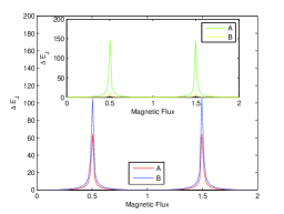
Figure 3: Shift of the Josephson coupling ($\Delta E_{J}$) due to the magnetic flux induced dissipation effect with magnetic flux (measured with respect to magnetic flux quantum, ${{\phi}_{0}}=\frac{hc}{2e}$). The red line is for the shifting of the Josephson coupling for the phase boundary between the RL2 and the superconducting phase. Blue line is for the shift of the phase boundary between the CDW and RL1 phase. Inset shows the shift of the Josephson coupling for the particle-hole symmetric point (green line) and the Charge degeneracy point (yellow line) in the figure.

Figure 4: Dissipative quantum phase diagram ($E_{J}$ vs. $V_{g}$) of the SQD array. We have depicted the different phases of the model Hamiltonians by: A. Mott insulating phase, B. Charge-density wave (CDW); C. First kind of Repulsive Luttinger liquid (RL1); D. Second kind of Repulsive Luttinger liquid (RL2); E. Superconductivity. Q and P2 are the multi-critical points (please see the text). $K$ is 1 at the phase boundary between Luttinger liquid (RL2) and superconductivity and also at the phase boundary between Mott phase and superconductivity. $K=1/4$ at the phase boundary between RL1 and CDW state. $K=2$ and $1/2$ at the $P1$ and $Q$ point respectively. $Q$ and $P1$ are the special points, $Q$ is the charge degeneracy point and $P1$ is the particle-hole symmetric point. We notice that due to the dissipation, phase boundaries and special points are shifted w.r.t Josephson coupling, please see the text for detail explanation.

III 3. Quantum Field Theoretical Study of Model Hamiltonian of The System and Explicit Derivation of Dissipative Strength

In the previous section and also from our previous study suj2 , we have shown explicitly that the mesoscopic SQUIDs array is equivalent to the array of superconducting quantum dots (SQD) array with modulated Josephson coupling. We first write the model Hamiltonian of SQD with nearest neighbor (NN) Josephson coupling Hamiltonian ($H_{J1}$) and also with the presence of the on-site ($H_{EC0}$) and NN charging energy ($H_{EC1}$) between SQD as,

$$H~{}=~{}H_{J1}~{}+~{}H_{EC0}~{}+~{}H_{EC1}.$$ (14)

We would like to recast our model Hamiltonian in the magnetic flux induced Coulomb blocked regime (${E_{C0}}>>{E_{J}}$). In this regime, one can recast the Hamiltonian in spin operators. It is also observed from the experiments that the quantum critical point exists for larger values of the magnetic field, when the magnetic field induced Coulomb blockade phase is more prominent than the $E_{J}$ induced SC phase. Thus our theoretical model is consistent with the experimental findings. During this mapping process we follow Ref. (lar ; suj1 ; suj2 ), so that.

$$H_{J1}~{}=~{}-2~{}E_{J1}\sum_{i}({S_{i}}^{\dagger}{S_{i+1}}^{-}+h.c)$$

, ${E_{J1}}={E_{J}}|cos(\frac{\pi\Phi}{{\Phi}_{0}})|$,

$$H_{EC0}~{}=~{}\frac{E_{C0}}{2}\sum_{i}{({S_{i}}^{Z}-h)}^{2}.$$

are the Hamiltonian $H_{EC0}$ accounts for the influence of gate voltage ($eN\sim V_{g}$), where $eN$ is the average dot charge induced by the gate voltage. When the ratio $\frac{E_{J1}}{E_{C0}}\rightarrow 0$, the SQD array is in the insulating state having a gap of the width $\sim{E_{C0}}$, since it costs an energy $\sim E_{C0}$ to change the number of pairs at any dot. The exceptions are the discrete points at $N~{}=~{}(2n+1)$, where a dot with charge $2ne$ and $2(n+1)e$ has the same energy because the gate charge compensates the charges of extra Cooper pair in the dot. On this degeneracy point, a small amount of Josephson coupling leads the system to the superconducting state. Here $h=\frac{N-2n-1}{2}$ allows the tuning of the system around the degeneracy point by means of gate voltage. $H_{EC1}~{}=~{}4E_{Z1}\sum_{i}{S_{i}}^{Z}~{}{S_{i+1}}^{Z}$ . At the Coulomb blocked regime, the higher order expansion leads to the virtual state with energies exceeding $E_{C0}$. In this second order process, the effective Hamiltonian reduces to the subspace of charges $0$ and $2$, and takes the form lar ; suj1 ; suj2 ,

$$H_{C}~{}=~{}-\frac{3{E_{J1}}^{2}}{4E_{C0}}\sum_{i}{{S_{i}}^{Z}}{{S_{i+1}}^{Z}}~{}-~{}\frac{{E_{J1}}^{2}}{E_{C0}}\sum_{i}({S_{i+2}}^{\dagger}{S_{i}}^{-}+h.c).$$ (15)

With this corrections $H_{EC1}$ become

$$H_{EC1}~{}\simeq~{}(4E_{Z1}~{}-~{}\frac{3{E_{J1}}^{2}}{4E_{C0}})~{}\sum_{i}{{S_{i}}^{Z}}{{S_{i+1}}^{Z}}.$$

In this analytical expression, we only consider the nearest -neighbor contribution of the interaction. There is no evidence of next-nearest-neighbour interaction for mesoscopic SQUID array system havi3 . One can express spin chain systems to as spinless fermions systems through the application of Jordan-Wigner transformation. In Jordan-Wigner transformation the relation between the spin and the electron creation and annihilation operators are $S^{z}(x)=\psi^{\dagger}(x)\psi(x)-1/2$, $S^{-}(x)={\psi(x)}~{}\exp[i\pi\sum_{j=-\infty}^{x-1}n_{j}]$, where $S^{+}={(S^{-})}^{+},n(x)={\psi^{\dagger}}(x){\psi(x)}$ is the fermion number at the site $x$. We have transformed all Hamiltonians in spinless fermions as follows: $H_{J1}~{}=~{}-2~{}E_{J1}\sum_{i}({{\psi}_{i}}^{\dagger}{{\psi}_{i+1}}^{-}+h.c)$, $H_{EC0}~{}=~{}2h{E_{C0}}\sum_{i}({{\psi}_{i}}^{\dagger}{{\psi}_{i}}-1/2).$ $H_{EC1}~{}\simeq~{}(4E_{Z1}~{}-~{}\frac{3{E_{J1}}^{2}}{4E_{C0}})~{}\sum_{i}({{\psi}_{i}}^{\dagger}{{\psi}_{i}}-1/2)({{\psi}_{i+1}}^{\dagger}{{\psi}_{i+1}}-1/2).$

In order to study the continuum field theory of these Hamiltonians, we recast the spinless fermions operators in terms of field operators by a relation gia2 .

$${\psi}(x)~{}=~{}~{}[e^{ik_{F}x}~{}{\psi}_{R}(x)~{}+~{}e^{-ik_{F}x}~{}{\psi}_{L}(x)]$$ (16)

where ${\psi}_{R}(x)$ and ${\psi}_{L}(x)$ describe the second-quantized fields of right- and the left-moving fermions respectively. We would like to express the fermionic fields in terms of bosonic field by the relation

$${{\psi}_{r}}(x)~{}=~{}~{}\frac{U_{r}}{\sqrt{2\pi\alpha}}~{}~{}e^{-i~{}(r\phi(x)~{}-~{}\theta(x))},$$ (17)

where $r$ denotes the chirality of the fermionic fields, right (1) or left movers (-1). The operators $U_{r}$ preserve the anti-commutivity of fermionic fields. $\phi$ field corresponds to the quantum fluctuations (bosonic) of spin and $\theta$ is the dual field of $\phi$. They are related by the relations ${\phi}_{R}~{}=~{}~{}\theta~{}-~{}\phi$ and ${\phi}_{L}~{}=~{}~{}\theta~{}+~{}\phi$. The Hamiltonians without ($H_{1}$) and with co-tunneling ($H_{2}$) effect are the following

$$H_{1} = {H_{0}}+\frac{4E_{Z1}}{{(2\pi\alpha)}^{2}}\int~{}dx:cos(4\sqrt{K}\phi(x)):$$ (18)

$$+\frac{E_{C0}}{\pi\alpha}\int({{\partial}_{x}}\phi(x))~{}dx$$

$$H_{2} = {H_{0}}+\frac{(4E_{Z1}-\frac{3{E_{J1}}^{2}}{4E_{C0}})}{{(2\pi\alpha)}^{2}}\int~{}dx:cos(4\sqrt{K}\phi(x)):$$ (19)

$$+\frac{E_{C0}}{\pi\alpha}\int({{\partial}_{x}}\phi(x))~{}dx$$

Where, $H_{0}$ is the non-interacting part of the Hamiltonian. The Luttinger liquid parameters of the Hamiltonian $H_{1}$ and $H_{2}$ are $K_{1}$ and $K_{2}$ are respectively.

$${K_{1}}~{}=~{}\frac{\pi}{\pi~{}+~{}2sin^{-1}{\Delta}_{1}}$$ (20)

$${K}_{2}~{}=~{}\frac{\pi}{\pi~{}+~{}2sin^{-1}{\Delta}_{2}}$$ (21)

${{\Delta}_{1}}=\frac{2E_{Z1}}{E_{J1}}$ ${{\Delta}_{2}}=\frac{2E_{Z1}}{E_{J1}}~{}-~{}\frac{3{E_{J1}}}{8E_{C0}}$. We calculate the dissipation strength by calculating K for both cases and then we use the relation $K=4{\alpha}$. Therefore the dissipative strength in absence (${{\alpha}_{1}}$) and presence (${{\alpha}_{2}}$) of co-tunneling effect are

$${{\alpha}_{1}}~{}=~{}\frac{1}{4}\frac{\pi}{\pi~{}+~{}2sin^{-1}{\Delta}_{1}}$$ (22)

$${{\alpha}_{2}}~{}=~{}\frac{1}{4}\frac{\pi}{\pi~{}+~{}2sin^{-1}{\Delta}_{2}}$$ (23)

This is the first analytical derivation of flux induced dissipation strength in terms of the interactions of the system. In the derivation of $K_{2}$ and ${\alpha}_{2}$, we only consider the nearest- neighbour hopping consideration when we consider the effect co-tunneling. We consider these two processes to emphasis the importance of co-tunneling effect for this system. Before we proceed further for the analysis of the Hamiltonian , $H_{1}$ and $H_{2}$, we want to explain in detail for the different values of $K$ at the different points (like P1, Q and P2) of phase diagram and also at the phase boundaries. The physical analysis of the phases and clear distinction of the phase boundaries will depend on the values of the K. Point Q is the charge degeneracy point for the low Cooper-pair density ($n_{i}=1/2$). The value of $K$ will be evaluated from the relevance of sine-Gordon terms. At the point Q, system is in the second order commensurability, sine-Gordon coupling terms ,Eq. 18 and Eq. 19, will become relevant for $K=1/2$, which is depicted in the Fig.1. Point P1 is the particle hole symmetric point, i.e., there is one particle in each site. At this point system is in the first order commensurability, i.e., the sine-Gordon coupling term is $cos(2\sqrt{K}\phi(x))$. So this term will become relevant for K=2, which is depicted in the Fig.1. We are understanding from Eq. 18 and Eq. 19 that the applied gate voltage acts as a chemical potential. So the proper tuning of gate voltage will drive the system from the insulating state to the other quantum phases of the system. We are now interested in finding the value of K at the phase boundaries, hence analysis is the following: We follow the Luther-Emery luth trick during the analysis. One can write the sine-Gordon Hamiltonian for arbitrary commensurability as

$$H_{3}~{}=~{}H_{0}~{}+~{}\lambda\int~{}dx~{}cos(2n\sqrt{K}\phi(x)),$$ (24)

where $n$ is the commensurability and $\lambda$ is the coupling strength. $H_{0}$ is the free part of the Hamiltonian. We know that for the spinless fermions, ${{\psi}_{R}}^{\dagger}{{\psi}_{L}}~{}+~{}{{\psi}_{L}}^{\dagger}{{\psi}_{R}}~{}=~{}\frac{1}{{2\pi a}^{2}}\int dxcos(2\sqrt{K}\phi(x))$, which is similar to the analytical expression of sine-Gordon coupling term but with the wrong coefficient inside the cosine. One can set ${\tilde{\phi}(x)}~{}=~{}2\sqrt{\tilde{K}}\phi(x)$ then the Eq. 24 become

$$H_{4}~{}=~{}H_{0}+\lambda\int~{}dxcos(2{\tilde{\phi}(x)}).$$ (25)

$K$ and $\tilde{K}$ are related by the relation, $K~{}=~{}\frac{\tilde{K}}{n^{2}}$.

At the phase boundary, $\tilde{K}~{}=1$ that implies $K=1/n^{2}$. So for the first and second order commensurability the value of $K$ at the phase boundary are 1 and 1/4 respectively which is depicted in Fig. 1. The point to be noticed that if we start from an initial model with $K~{}=~{}1/n^{2}$, i.e., in general a strongly interacting model, the resulting spin-less fermions model corresponds in the boson language to $K=1$ which means that it is non-interacting. For this particular value of $K$ the spin-less fermions whose bosonized form is Eq. 25 are just free particle with backscattering. This special value of $K$ is known as the Luther-Emery luth line, the importance of the Luther-Emery solution is to provide a solution for the massive phase on the whole line $K=1/n^{2}$ for arbitrary $\lambda$.
Here we do the analysis for Hamiltonian $H_{1}$. In the limit $\Delta~{}=~{}{\Delta}_{1}$, for $E_{J}<2E_{Z1}$ and relatively small field, the anti-ferromagnetic Ising interaction dominate the physics of anisotropic Heisenberg chain. When the field is large, i.e., the applied gate voltage is large, the chain state is in the ferromagnetic state. In the language of interacting bosons, The Neel phase is the commensurate charge density wave phase with period 2, i.e., there is only one boson in every two sites. In Fig. 1 this phase region is described by region B. The ferromagnetic state is the Mott insulating state, this is the phase A of our quantum phase diagram (Fig. 1). $H_{1}$ is the Heisenberg XXZ model Hamiltonian in a magnetic field. The emergence of two Luttinger liquid phases for the following reasons: RL1 and RL2 respectively occur due to commensurate-incommensurate transition and the criticality of Heisenberg XY model. For the intermediate values of the field, system is either in the first kind of repulsive Luttinger liquid (RL1) phase for $K<1/2$ or in the second kind of repulsive Luttinger liquid (RL2) phase for $K>1/2$. The physical significance of RL1 phase is that the coupling term is relevant but the applied magnetic field, i.e., the applied gate voltage on the dot, breaks the gapped phase whereas in the RL2 phase non of the coupling term is relevant due to the larger values of $K$ ($>1/2$). The phase regions are described by C and D respectively for the RL1 and RL2 in Fig.2. These phase regions in Fig. 2, are all most same for two different limits, $\Delta={\Delta}_{1}$ and $\Delta={\Delta}_{2}$. So we predict the existence of two RL from two different sources. In previous studies this clarification was absent and they had reported only one RL lar . The value of $K=1$ at the phase boundary between the MI and SC phase and also between the RL2 and SC phase. From the analysis of $K$ at the phase boundary we obtain $E_{Z1}=0$, according to our theory and also from the experimental findings this condition is unphysical. So the interaction space of Hamiltonian $H_{1}$ is not sufficient to produce the whole phase diagram of Fig. 2. It indicates that we shall have to consider more extended interaction space to get the correct phase diagram. If we consider the co-tunneling effect in this Hamiltonian system, i.e., the Hamiltonian $H_{2}$. The phase boundary analysis at the MI and SC phase and also for the RL2 and SC phase implies that we get the condition $E_{J1}~{}=~{}\sqrt{\frac{16E_{Z1}E_{C0}}{3}}$, which is consistent physically. Now we discuss the effect of magnetic field induced dissipation on the quantum phase diagram of superconducting quantum dot lattice. We have already proven in the previous section the analytical relation between the LL parameter ($K$) and the dissipation strength in presence of magnetic flux. Here we use the analytical expression for $K$ to study the effect of magnetic flux on the quantum phases and quantum phase boundaries. Therefore the modified quantum phase diagram in presence of magnetic flux include the magnetic flux induce dissipation effect. In the previous paragraph we emphasis the importance of co-tunneling effect. Therefore we consider the Eq.(21) and Eq.(23) when we consider the shift of the Josephson couplings due to the presence of magnetic flux induced dissipation. It is very clear from Eq. 21 and Eq. 23 that the analytical relation of the Josephson coupling with the system interactions parameters at different phase boundaries and different points are more complicated than the Ambegaokar and Baratoff relation ambe . The analytical expression for the Josephson couplings at the different phase boundaries and special points are the following:
Particle-Hole symmetric point ($K=2$),

$$E_{J}~{}=~{}0.9428{E_{C0}}(\sqrt{1+\frac{6E_{Z1}}{E_{C0}}}+1)$$ (26)

Charge-Degeneracy point $(K=1/2)$,

$$E_{J}~{}=~{}{0.75E_{C0}}(\sqrt{1+\frac{3E_{Z1}}{E_{C0}}}-1)$$ (27)

Phase boundary between the RL2 and SC phase $(K=1)$,

$$E_{J}~{}=~{}{4}(\sqrt{\frac{E_{Z1}E_{C0}}{3}})$$ (28)

Phase boundary between CDW state RL1 phase $(K=1/4)$,

$$\Delta E_{J}~{}=~{}{0.75E_{C0}}(\sqrt{1+\frac{3E_{Z1}}{E_{C0}}}+1).$$ (29)

Our main intension is to study the effect of magnetic flux on the particle hole symmetric point ($K=2$ ), charge degeneracy point ($K=1$), multicritical point and also for the phase boundaries between the different quantum phases.
The analytical expressions for the shift of Josephson couplings ($\Delta E_{J}$) due to the presence of magnetic flux are the following:
Particle-Hole symmetric point ($\alpha=1/2$),

$$\Delta E_{J}~{}=~{}0.9428{E_{C0}}(\sqrt{1+\frac{6E_{Z1}}{E_{C0}}}+1)(1/|cos(\frac{\pi\phi}{{\phi}_{0}})|-1)$$ (30)

Charge-Degeneracy point $(\alpha=1/8)$,

$$\Delta E_{J}~{}=~{}{0.75E_{C0}}(\sqrt{1+\frac{3E_{Z1}}{E_{C0}}}-1)(1/|cos(\frac{\pi\phi}{{\phi}_{0}})|-1)$$ (31)

Phase boundary between the RL2 and SC phase $(\alpha=1/4)$,

$$\Delta E_{J}~{}=~{}{4}(\sqrt{\frac{E_{Z1}E_{C0}}{3}})(1/|cos(\frac{\pi\phi}{{\phi}_{0}})|-1)$$ (32)

Phase boundary between CDW state RL1 phase $(\alpha=1/16)$,

$$\Delta E_{J}~{}=~{}{0.75E_{C0}}(\sqrt{1+\frac{3E_{Z1}}{E_{C0}}}+1)(1/|cos(\frac{\pi\phi}{{\phi}_{0}})|-1)$$ (33)

In Fig. 3, we present our results of deviation of Josephson coupling as a function of magnetic flux. We observe that this deviation is maximum at the half-integers values of magnetic flux quantum. It reveals from our study that the effect of magnetic flux induce dissipation for the half-integer values of magnetic flux quantum is slightly prominant for the special points compare to the qunatum phase boundaries. Inset shows the shift of Josephson coupling for the particle-hole symmetric point and the charge degeneracy point. It is also clear from the inset that the magnetic flux induce dissipation is more prominant for the particle-hole symmetric point compare to the charge degeneracy point.
It is very clear from the analytical expression from Eq. 30 to Eq. 33 and also from the Fig.3 from our study that there is no appreciable changes in the quantum phase diagram for small magnetic flux in the system. As the applied magnetic fluxes changes from $0.4{\phi}_{0}$ to $0.6{\phi}_{0}$, quantum phase diagram shows some appreciable change and it is robust for the half-integer magnetic flux quantum.
In Fig. 4, we present the magnetic flux induce dissipative quantum phase diagram of our system. This schematic phase diagram is for values of magnetic flux which appreciably effect the phase boundaries and special points as we have discussed in the previous paragraph. We present the phase boundaries and special points in terms of the dissipative strength of the system. We observe from our study that magnetic flux induce dissipation favour the insulating phase and the gapless LL phase over the superconducting phase of the system which is consistent with the experimental findings [13].

IV summary and conclusions

We have studied the quantum phase diagram of mesoscopic SQUID array in absence and presence of magnetic flux. The magnetic flux induced dissipation modified quantum phase diagram of our system. We have derived an analytical relation between the Luttinger liquid parameter and dissipation strength. We have also noticed that magnetic flux induced dissipation effect is not same for all values of magnetic flux quantum. We have also observed that the magnetic flux induce dissipation favours the insulating phase of the system over the Luttinger liquid and superconducting phase of the system.
Acknowledgement: The author would like to acknowledge Dr. N. Sundaram for reading the manuscript critically.

References

- (1) G. Schon and A. D. Zaikin, Physics Reports 198, 237 (1990)
- (2) R. Fazio and H. van der Zant, Physics Reports 355, 235 (2001).
- (3) D. B. Haviland, Y. Liu, and A. M. Goldman, Phys. Rev. Lett. 62, 2180 (1989).
- (4) N. Mason and A. Kapitulink, Phys. Rev. Lett 82, 5341 (1999); N. Mason and A. Kapitulnik, Phys. Rev. B 65, 220505 (2002).
- (5) A. Bezryadin, C. N. Lau and M. Tinkham, Nature 404, 971 (2002).
- (6) A. Bezryadin, J. Phys Condens Matter 20, 043202 (2008).
- (7) S. L. Sondhi , Rev. Mod. Phys. 69, 315 (1997).
- (8) L. I. Glazmann , Phys. Rev. Lett. 39, (1997) 3786.
- (9) S. Sarkar, Phys. Rev. B 75, 014528 (2007); Euro. Phys. Lett, 71 (2005) 980.
- (10) S. Sarkar, Eur. Phys. J. B 67, 559 (2009).
- (11) L. J. Geerligs , Phys. Rev. Lett. 63, 326 (1989).
- (12) H. S. J. van der Zant , Euro. Phys. Lett. 119, 541 (1992).
- (13) E. Chow , Phys. Rev. Lett. 81, 204 (1998).
- (14) W. Kuo , Phys. Rev. Lett. 87, 186804 (2001).
- (15) E. Granto , Phys. Rev. Lett. 65, 1267 (1990).
- (16) C. D. Chen , Phys. Rev. B 51, 15645 (1995).
- (17) G. Refael, E. Demler, Y. Oreg and D. S. Fisher, Phys. Rev. B 75, 014522 (2007).
- (18) A. M. Lobos and T. Giamarchi, Phys. Rev. B 84, 024523 (2011).
- (19) A. O. Calderia, A. J. Leggett, Phys. Rev. Lett 46, 211 (1981).
- (20) A. Schmid, Phys. Rev. Lett. 51, 1506 (1983).
- (21) S. Chakravarty , Phys. Rev. B 37, 3238 (1988).
- (22) P. Goswami and S. Chakravarty, Phys. Rev. B 73, 094516 (2006).
- (23) S. Schon and A. D. Zaikin, Phys. Reports 198, 237 (1990).
- (24) C. Kane and M. P. A Fisher, Phys. Rev. B 46, 15233 (1992).
- (25) A. Furusaki and N. Nagaosa, Phys. Rev. B 47, 4631 (1993) ; ibid Phys. Rev. B 47, 3827 (1993).
- (26) D. S. Golubev and A. D. Zaikin, Phys. Rev. B, 64 014504 (2001); A. D. Zaikin , Phys. Rev. Lett., 78 1552 (1997).
- (27) V. Ambegaokar and A. Baratoff, Phys. Rev. Lett 10, 486 (1963).
- (28) M. A. Cazalilla, F. Solus and F. Guinea, Phys. Rev. Lett 97, 076401 (2006).
- (29) A. Luther and V. J. Emery, Phys. Rev. Lett 33, 589 (1974).
- (30) T. Giamarchi, in Quantum Physics in One Dimension (Claredon Press, Oxford 2004).