Stability and chaos of hierarchical three black hole configurations

Abstract

We study the stability and chaos of three compact objects using post-Newtonian (PN) equations of motion derived from the Arnowitt-Deser-Misner-Hamiltonian formulation. We include terms up to 2.5 PN order in the orbital part and the leading order in spin corrections. We performed numerical simulations of a hierarchical configuration of three compact bodies in which a binary system is perturbed by a third, lighter body initially positioned far away from the binary. The relative importance of the different PN orders is examined. The basin boundary method and the computation of Lyapunov exponent were employed to analyze the stability and chaotic properties of the system. The 1 PN terms produced a small but noticeable change in the stability regions of the parameters considered. The inclusion of spin or gravitational radiation does not produced a significant change with respect to the inclusion of the 1 PN terms.

I Introduction

The dynamics of compact objects play an important role in the evolution of galaxies and other stellar systems. Post-Newtonian (PN) techniques are a useful tool for modeling the dynamics of multiple compact objects. In astrophysical models, the gravitational radiation is included via an effective force which considers 1 PN and 2.5 PN corrections, and in some cases stellar dynamical friction. Hierarchical three black hole configurations interacting in a galactic core have been the focus of recent studies by several authors. For example, intermediate-mass black holes with different mass ratios are considered in GulMilHam03 ; GulMilHam04 ; GulMilHam05a ; simulations of dynamical evolution of triple equal-mass supermassive black holes in a galactic nuclei were performed in IwaFunMak06 ; HofLoe07 . Other astrophysical applications of multiple black hole simulations include three-body kicks Hofloe06 ; GuaPorSip05 and binary-binary encounters (see e.g. Mik83 ; Mik84 ; MilHam02 ; Hei01 ; ValMik91 ). In the context of the final parsec problem MilMer03 ; ValMikHei94 , three-body interactions are considered as a mechanism that can drive a binary black holes system to a separation below one parsec.

Since the 1990s there has been an increasing effort to detect and study compact objects. The most likely source of gravitational waves are binary compact objects. Recently, it was shown that the probability of more than two black holes to interact in the strongly relativistic regime is, not surprisingly, very small AmaDew10 . For practical purposes, the creation of gravitational waveform templates for gravitational wave detectors is naturally focused on binary systems. Binary systems can produced complicate waveforms when taking into account spinning black holes and eccentric orbits, e.g. LevCon10 . On the other hand, triple systems consisting of a binary black hole and a star (e.g., a white dwarf) are potential sources of electromagnetic counterparts associated with the mergers SetMut10 ; SetMut11 ; StoLoe10 ; CheSesMad11 .

The chaotic behavior of triple systems is well known in the Newtonian case (see ValKar06 and references therein). For binaries, it is known that chaos appears when using certain post-Newtonian approximations for spinning binary systems (see Lev00 ; CorLev03 ; BarLev03 ; Lev06 ; GopKni05 ; Han08 ; SchRas01 ). In the present work, we studied three-body systems with PN methods, where the main technical novelty is the inclusion of the 2.5 PN terms in the orbital dynamics and leading order of spin-orbit and spin-spin terms DamJarSch07a ; SteHerSch08 ; HarSte11 .

Recently, similar PN techniques were applied to the general relativistic three-body problem. Periodic solutions were studied using the 1 PN and 2 PN approximations in Moo93 ; TatTakHid07 ; LouNak08 . Examples of three compact bodies in a collinear configuration were considered in YamAsa10 ; YamAsa10a , and Lagrange’s equilateral triangular solution was studied including 1 PN effects in IchYamAsa10 . In JSch10 , the stability of the Lagrangian points in a black hole binary system was studied in the test particle limit, where the gravitational radiation effects were modeled by a drag force. The waveform characterization of hierarchical non-spinning three-body configurations using up to 2.5 PN terms was presented in GalBru11 .

Close interaction and merger of black holes require numerical relativistic simulations. The first complete simulations, using general-relativistic numerical evolutions of three black holes, were presented in CamLouZlo07f ; LouZlo07a . These recent simulations showed that three compact object dynamics display a qualitatively different behavior than Newtonian dynamics. In GalBruCao10a , the sensitivity of fully relativistic evolutions of three and four black holes to changes in the initial data was examined, where the examples for three black holes are some of the simpler cases already discussed in CamLouZlo07f ; LouZlo07a . The apparent horizon and the event horizon of multiple black holes have been studied in Die03a ; JarLou10 ; PonLouZlo10 . Although fully general-relativistic simulations are available, they are constrained by the number of orbits and separations between black holes.

The paper is organized as follows: in Sec. II, we summarize the equation of motion up to 2.5 post-Newtonian approximation for three spinning bodies. This is followed by a discussion of the chaos indicators that we used to characterize the triple system. In Sec. III.1, we describe the numerical techniques used to solve the equation of motion, and we present some results for test cases. The perturbation of a binary system by a third object is presented in Sec. III.2, where we performed numerical experiments in order to study the stability and chaos of the triple system. The conclusions are presented in Sec. IV.

I.1 Notation and units

We employed the following notation: $\vec{x}=(x_{i})$ denotes a point in the three-dimensional Euclidean space $\mathbb{R}^{3}$ and letters $a,b,\dots$ are the particle labels. We defined $\vec{r}_{a}:=\vec{x}-\vec{x}_{a}$, $r_{a}:=|\vec{r}_{a}|$, $\hat{n}_{a}:=\vec{r}_{a}/r_{a}$; for $a\neq b$, $\vec{r}_{ab}:=\vec{x}_{a}-\vec{x}_{b}$, $r_{ab}:=|\vec{r}_{ab}|$ and $\hat{n}_{ab}:=\vec{r}_{ab}/r_{ab}$; here, $|\cdot|$ denotes the length of a vector. The mass parameter of the $a$-th particle is denoted by $m_{a}$ with $M=\sum_{a}m_{a}$. Summation runs from 1 to 3. The linear momentum vector is denoted by $\vec{p}_{a}$. A dot over a symbol, $\dot{\vec{x}}$, means the total time derivative, and the partial differentiation with respect to $x^{i}$ is denoted by $\partial_{i}$.

In order to simplify the calculations, it is useful to define dimensionless variables (see e.g.  Szi06 ). We used as basis quantities for the Newtonian and post-Newtonian calculation the gravitational constant $G$, the speed of light $c$ and the total mass of the system $M$. Using derived constants for time $\tau=MG/c^{3}$, length $\mathit{l}=MG/c^{2}$, linear momentum $\mathcal{P}=Mc$, spin $\mathcal{S}=M^{2}G/c$ and energy $\mathcal{E}=Mc^{2}$, we construct dimensionless variables. The physical variables are related to the dimensionless variables by means of scaling. Denoting with capital letters the physical variables with the standard dimensions and with lowercase the dimensionless variables. We defined for a particle $a$ its position $\vec{x}_{a}:=\vec{X}_{a}/\mathit{l}$, linear momentum $\vec{p}_{a}:=\vec{P}_{a}/\mathcal{P}$ and mass $m_{a}=M_{a}/M$ (notice that $m_{a}<1$, $\forall a$).

II Evolution method

II.1 Equations of motion

In the ADM post-Newtonian approach, it is possible to split the orbital and spin contribution to the Hamiltonian (see e.g. Bla06a ; Mag07a )

$$H(\vec{x}_{a},\vec{p}_{a},\vec{s}_{a})=H(\vec{x}_{a},\vec{p}_{a})_{\mathrm{Orb}}+H(\vec{x}_{a},\vec{p}_{a},\vec{s}_{a})_{\mathrm{Spin}},$$ (1)

where each component forms a series with coefficients which are inverse powers of the speed of light. We included terms up to 2.5 PN contributions where the orbital part for three bodies is given by Sch87 ; LouNak08 ; GalBru11

$$H_{\mathrm{Orb}}=H^{(0)}_{\mathrm{N}}+H^{(1)}_{\mathrm{PN}}+H^{(2)}_{\mathrm{PN}}+H^{(2.5)}_{\mathrm{PN}}.$$ (2)

Here each term of the Hamiltonian is labeled by a superscript $n$ that denotes the PN order (powers of $c^{-2n}$) and a subscript which distinguished between the Newtonian terms and the PN components. The spin contribution forms a power series where the leading order is given by DamJarSch99 ; DamJarSch00b ; DamJarSch00c ; DamJarSch01 (see HarSte11 for the next-to-leading order terms)

$$H_{\mathrm{Spin}}=H^{\mathrm{LO}}_{\mathrm{SO}}+H^{\mathrm{LO}}_{\mathrm{SS}}+H^{\mathrm{LO}}_{\mathrm{S}^{2}}.$$ (3)

In this case, the superscripts denote the leading order terms ($\mathrm{LO}$) while the subscript distinguishes the kind of interaction: spin-orbit ($\mathrm{SO}$), spin(a)-spin(b) ($\mathrm{SS}$) or spin(a)-spin(a) ($\mathrm{S}^{2}$). We specified the initial spin of the particles by using a dimensionless parameter $\chi_{a}\in[0,1]$ and the two spherical angles $\theta_{a}$ and $\phi_{a}$. The initial spin of the particles is given by

$$\vec{s}_{a}(0)=\chi_{a}m^{2}_{a}(\cos\phi_{a}\sin\theta_{a}\hat{x}+\sin\phi_{a}\sin\theta_{a}\hat{y}+\cos\theta_{a}\hat{z}),$$ (4)

where $\hat{x}$, $\hat{y}$ and $\hat{z}$ are the unitary basis vectors in Cartesian coordinates. Using the Hamiltonian (1), the equations of motion are

$$\dot{x}^{i}_{a} = \frac{\partial H}{\partial p^{i}_{a}},$$ (5)

$$-\dot{p}^{i}_{a} = \frac{\partial H}{\partial x^{i}_{a}},$$ (6)

$$\dot{s}^{i}_{a} = \frac{\partial H}{\partial s^{j}_{a}}s_{a}^{k}\epsilon_{ijk}.$$ (7)

The first term in (2) is the Hamiltonian for $n$-particles interacting under Newtonian gravity

$$H^{(0)}_{N}=\frac{1}{2}\sum^{n}_{a}\frac{\vec{p}_{a}^{\;2}}{m_{a}}-\frac{1}{2}\sum^{n}_{a,b\neq a}\frac{m_{a}m_{b}}{r_{ab}}.$$ (8)

The explicit form of the PN terms in (2) and the equation of motion for three compact objects can be found in GalBru11 (see also Sch87 ; LouNak08 ). The spinning part terms (3) for $n$ compact objects are given in HarSte11 .

We will refer as Newtonian, 1 PN, 2 PN and 2.5 PN to the equations of motion derived from $H^{(0)}_{\mathrm{N}}$, $H^{(0)}_{\mathrm{N}}+H^{(1)}_{\mathrm{PN}}$, $H^{(0)}_{\mathrm{N}}+H^{(1)}_{\mathrm{PN}}+H^{(2)}_{\mathrm{PN}}$ and $H^{(0)}_{\mathrm{N}}+H^{(1)}_{\mathrm{PN}}+H^{(2)}_{\mathrm{PN}}+H^{(2.5)}_{\mathrm{PN}}$, respectively. We denoted as radiative Newtonian and radiative 1 PN the equations of motion derived from $H^{(0)}_{\mathrm{N}}+H^{(2.5)}_{\mathrm{PN}}$ and $H^{(0)}_{\mathrm{N}}+H^{(1)}_{\mathrm{PN}}+H^{(2.5)}_{\mathrm{PN}}$, respectively.

II.2 Chaos indicators

There are a number of methods for diagnosing chaos in a dynamical system: the Poincaré surface (for system with less than 3 degrees of freedom), the Kolmogorov-Sinai entropy, the characteristic Lyapunov exponent and the fractal basin boundary method, among others (see e.g.  EckRue85 ; WuXie08 ; McDGreOtt85 ). For our analysis, we employed the fractal basin boundary method and the Lyapunov exponent. In this section, we describe the implementation of both methods.

The basin boundary method and the Lyapunov exponents are able to characterize different types of chaos. The basin boundary characterizes the sensitive dependence on initial conditions for nearby orbits with different attractors on the phase-space. However, it does not provide information about the orbit itself. Alternatively, the Lyapunov indicator characterizes the regularity or chaos of an orbit in a way that is independent from the attractor.

II.2.1 Fractal basin boundary

A dynamical system usually exhibits a transient behavior followed by an asymptotic regime. The time-asymptotic behavior defines attracting sets in the phase-space which are called attractors. The attractor can be periodic, quasi-periodic or chaotic. The closure of the set of initial conditions, which has a particular attractor, is called basin of attraction. Basin boundaries for a typical dynamical system can be either smooth or fractal McDGreOtt85 ; FarOttYor83 . A system with fractal basin boundaries is sensitive to initial uncertainty. Given $\epsilon>0$, we call the initial condition point $P^{*}$ unsafe if there is another initial condition point $P$ inside a neighborhood of size $\epsilon$ centered at $P^{*}$ which converges to a different attractor. The fraction $f$ of unsafe points is related to $\epsilon$ by

$$f(\epsilon)\sim\epsilon^{D-\mathrm{d}_{f}},$$ (9)

where $D$ is the dimension of the phase-space and $\mathrm{d}_{f}$ is the dimension of the basin boundary (see McDGreOtt85 ; PeiJurSau93 for a detailed discussion). It is useful to define an uncertainty exponent $\alpha=D-\mathrm{d}_{f}$, which satisfies the relation $0<\alpha\leq 1$. The value of $\alpha$ quantifies the presence of chaos in a basin boundary, $\alpha\approx 1$ for regular boundaries and $\alpha\approx 0$ for a chaotic region.

There are many ways of measuring the dimension of a fractal FarOttYor83 ; Fal90 . We employed the box-dimension which is defined as

$$\mathrm{d}_{\mathrm{box}}:=\lim_{\delta\rightarrow 0}\frac{\ln(N_{\delta}(A))}{\ln(1/\delta)},$$ (10)

where $A$ is a nonempty bounded set in the $\mathrm{d}_{E}$-dimensional Euclidean space and $N_{\delta}(A)$ is the smallest number of sets in a $\delta$-cover of $A$. A $\delta$-cover of $A$ is a collection of sets of diameter $\delta$ whose union contains $A$. For a physical or numerical experiment, the fractal basin boundary has finite resolution. A graphical representation of the basin boundary is given by an image formed by pixels of size $l_{\mathrm{res}}$. In order to estimate the dimension of the basin boundary, we compute the quotient $\ln(N_{\delta_{n}}(A))/\ln(1/\delta_{n})$ for a set of $\delta_{n}\geq l_{\mathrm{res}}$. The typical behavior of the resulting data is well approximated by a straight line. A linear regression method is used to fit a linear function to the resulting data (where $\delta_{n}=nl_{\mathrm{res}}$ and $n\in\{1,2,\dots,12\}$). Therefore, the value of the fitted function for $\delta=0$ gives an estimate value of the dimension. We tested the method by computing the dimension of non-fractal one-dimensional sets (i.e., a regular basin boundary) and Sierpinski’s gasket and carpet.

II.2.2 Lyapunov exponent

Lyapunov exponents are another way for characterizing chaos in a dynamical system (see e.g. EckRue85 ). For an autonomous $n$-dimensional system

$$\dot{\vec{X}}=\vec{F}(\vec{X}),$$ (11)

a given reference solution $\vec{X}_{*}$ and a nearby solution $\vec{X}=\vec{X}_{*}+\delta\vec{X}$. While the evolution of the difference $\delta\vec{X}$ is given by the linearized equation

$$\delta\dot{\vec{X}}=\mathbf{J}(\vec{X}_{*})\cdot\delta\vec{X},$$ (12)

where $\mathbf{J}(\vec{X}_{*})_{i,j}:=\partial_{j}F_{i}(\vec{X}_{*})$ is the Jacobian matrix of $\vec{F}$ evaluated at the reference solution $\vec{X}_{*}$. The solution of (12) is given by Arn78

$$\delta\vec{X}(t)=\mathbf{\mathrm{e}}^{\mathbf{J}t}\cdot\delta\vec{X}(0).$$ (13)

The Lyapunov exponents are defined by the eigenvalues $\Lambda_{i}(t)$ of the distortion matrix $\mathbf{\Lambda}:=\mathbf{\mathrm{e}}^{(\mathbf{J}+\mathbf{J}^{T})t}$

$$\lambda_{i}:=\lim_{t\rightarrow\infty}\frac{1}{2t}\ln\Lambda_{i}(t).$$ (14)

Sensitive dependence on initial conditions exists when $\lambda_{i}>0$. Therefore, in order to distinguish between regular and chaotic orbits, it is sufficient to compute the principal Lyapunov exponent $\lambda_{p}:=\max(\lambda_{i})$. Calculating $\lambda_{p}$ directly is computationally expensive. However, by using the evolution of the difference, $\delta\vec{X}$, it is possible to obtain an estimation of $\lambda_{p}$

$$\lambda^{*}_{p}:=\lim_{t\rightarrow\infty}\lim_{\delta X(0)\rightarrow 0}\lambda^{*}_{p}(t,\delta X(0)),\\$$ (15)

where,

$$\lambda^{*}_{p}(t,\delta X(0)):=\frac{1}{t}\ln\left(\frac{\delta X(t)}{\delta X(0)}\right),$$ (16)

and $\delta X(t)=|\delta\vec{X}|$. We will refer as a Lyapunov indicator to $\lambda^{*}_{p}$ in order to distinguish it from the principal Lyapunov exponent and the Lyapunov function, $\lambda^{*}_{p}(t,\delta X(0))$. The norm, $|\delta\vec{X}|$, plays an important role in the computation of the Lyapunov indicator. Particularly, in the case of general relativity, additional gauge effects can affect the estimation of the Lyapunov indicator CorLev03 ; WuXie08 ; WuHua03 . Results from literature were applied to general relativistic dynamic of test particles and to binary systems in the center of mass frame. Additionally, the estimation of $\lambda_{p}$ is often computed using the two-particle method instead of the evolution of the difference (see e.g. WuHuaZha06 ). However, we did not noticed significant differences in the computation of $\lambda^{*}_{p}$ given the gauge effects. We present the results in terms of the Cartesian length of $\delta\vec{X}$.

In practice, the Lyapunov indicator is computed approximating the limits, using a sufficient small $\delta\vec{X}(0)$ and sufficient large integration time. In our simulations, we used $|\delta\vec{X}(0)|=10^{-9}$. The integration time depends on the system (see Sec. III). The evolution is performed by solving numerically the system of equations (5)-(7), therefore $\vec{X}=(\vec{x}_{a},\vec{p}_{a},\vec{s}_{a})^{\mathrm{T}}$ is a vector with 27 components. The right hand side of (11) is the vector

$$\vec{F}=\left(\frac{\partial H}{\partial p^{i}_{a}},-\frac{\partial H}{\partial x^{i}_{a}},\frac{\partial H}{\partial s^{j}_{a}}s_{a}^{k}\epsilon_{ijk}\right),$$ (17)

and the equation of motion for the difference $\delta\vec{X}=(\delta\vec{x}_{a},\delta\vec{p}_{a},\delta\vec{s}_{a})$ is

$$\delta\dot{x}^{i}_{a} = \delta\vec{X}\cdot\nabla\frac{\partial H}{\partial p^{i}_{a}},$$ (18)

$$-\delta\dot{p}^{i}_{a} = \delta\vec{X}\cdot\nabla\frac{\partial H}{\partial x^{i}_{a}},$$ (19)

$$\delta\dot{s}^{i}_{a} = \delta\vec{X}\cdot\nabla\frac{\partial H}{\partial s^{j}_{a}}s_{a}^{k}\epsilon_{ijk},$$ (20)

where we define the auxiliary operator

$$\delta\vec{X}\cdot\nabla:=\sum^{3}_{b=1}\sum^{3}_{j=1}\left(\delta x^{j}_{b}\frac{\partial}{\partial x^{j}_{b}}+\delta p^{j}_{b}\frac{\partial}{\partial p^{j}_{b}}+\delta s^{j}_{b}\frac{\partial}{\partial s^{j}_{b}}\right).$$ (21)

III Simulations and results

III.1 Numerical methods

We solved the equations of motion numerically using the GNU Scientific Library (GSL) GalDavThe09 and the Olliptic code infrastructure GalBruCao10a . We generated the right hand side (RHS) of the equations of motion (5)-(7) with Mathematica 7.0 Wol08 .

The simulations were done using the embedded Runge-Kutta Prince-Dormand (8,9) method provided by the GSL. We used a scaled adaptive step-size control (see GalDavThe09 for details). In our simulations, the error control for the dynamical variables $(\vec{x}_{a},\vec{p}_{a},\vec{s}_{a})$ was set to $10^{-11}$ and to $10^{-6}$ for the variation variables $(\delta\vec{x}_{a},\delta\vec{p}_{a},\delta\vec{s}_{a})$. We used as an indicator of accuracy the estimate of the local error provided by the GSL routines and the conservation of the Hamiltonian for the simulations which do not included the radiation term.

For our stability analysis, we solved the system of equations (5)-(7) and (17)-(19) simultaneously. In order to perform the simulations in an efficient way, we adapted the number of variables depending on the problem. The parameters to consider are the number of bodies $nb$, the magnitude of the spin $\vec{s}_{a}$ and whether we are solving a planar or non-planar problem. As we mentioned before, the RHS of Eqs. (5)-(7) were generated by a Mathematica script. For the Newtonian case and 1 PN cases, it is convenient to compute the analytical expression for the RHS of Eqs. (18)-(20). The analytical expression for the 2 PN and the spinning cases produces large computational source files. The source file for the 2 PN is of 25 megabytes while the inclusion of the spin generates files over a hundred megabytes. The compilation and optimization of large files is not practical, since compilers run out of memory even in the 16 GB of RAM server that we tried. Therefore, for the 2 PN order and the spinning case we computed the RHS of Eqs. (18)-(20) numerically. In order to estimate the errors in the numerical computation of the Jacobian, we compared the results obtained for the Newtonian and 1 PN cases employing both methods (see Sec. III.1.1). The system (18)-(20) is the Jacobian matrix of (17). The problem reduces to the computation of

$$J_{i,j}=\frac{\partial F_{i}(\vec{X}_{*})}{\partial X^{j}}.$$ (22)

A simple 2nd, 4th and even 6th order finite difference method with a fix step size $h$ does not produce accurate solutions. The main issue is the nature of the components, for example, the position variables require a different optimal step-size than the momentum or the spin variables. We implemented an adaptive method based on the GSL differentiation routine. The method produces a solution with an estimated error below $10^{-8}$ (see Sec. III.1.1).

An important issue in the numerical integration of a three-body system arises when two of the bodies are very close to each other. In the case of adaptive step size methods, it is necessary to reduce the step size in order to resolve properly the orbits in the close interaction phase. A usual approach to deal with this problem is to perform a regularization of the equations of motion, see e.g., Bur67 ; Heg74 ; MikAar89 ; MikAar93 ; MikAar96 and references therein. However, in our simulations, we included a different criteria. Regardless of the equation of motion employed, we monitored the absolute value of each conservative part of the Hamiltonian (1) relative to the sum of the absolute values

$$H^{\%}_{i}:=100\left(\frac{|H_{i}|}{|H^{(0)}_{\mathrm{N}}|+|H^{(1)}_{\mathrm{PN}}|+|H^{(2)}_{\mathrm{PN}}|+L_{1}(H_{\mathrm{Spin}})}\right).$$ (23)

The simulations stop when the contribution of the first post-Newtonian correction is larger than 10%. We will refer to $H_{1}^{\%}>10\%$ as strong interaction. Empirical results showed that, for a similar configuration, the resulted waveform exhibits a growth characteristic of the merger phase GalBru11 . The dynamics after a strong interaction may lead to the merger of two of the bodies or to the escape of the lighter body. In order to determine safely whether there is a merger or not, it is necessary to employ full numerical relativistic simulation.

Additionally, we considered the Newtonian escape energy of each body in respect of the other two components

$$E^{a}_{\mathrm{esc}}:=\frac{1}{2}\mu_{a}\left(\frac{\vec{p}_{a}}{m_{a}}-\frac{\vec{p}^{\;*}_{a}}{m^{*}_{a}}\right)^{2}-\frac{\mu_{a}}{|\vec{x}_{a}-\vec{x}^{*}_{a}|},$$ (24)

where $\mu_{a}:=m_{a}m^{*}_{a}$, $m^{*}_{a}:=\sum_{b\neq a}m_{b}$, $\vec{x}^{*}_{a}:=(m^{*}_{a})^{-1}\sum_{b\neq a}m_{b}\vec{x_{b}}$ and $\vec{p}^{\;*}_{a}:=\sum_{b\neq a}\vec{p_{b}}$. The simulation stops when $E^{a}_{esc}>0$ for one of the bodies and the size of the system $S:=\sum_{a}|\vec{x}_{a}|$ is 100 times the initial size. During a close encounter of two of the bodies it is common to have a positive value of $E^{a}_{\mathrm{esc}}$ for a short time. However, imposing the second condition we exclude those cases. We performed several tests to estimate the numerical errors. Here we summarize the results of these tests.

III.1.1 Numerical tests

Our first test was done with Lagrange’s triangle solution using Newtonian equations of motion. In Lagrange’s solution each body is sitting in one corner of an equilateral triangle (see e.g. GolPooSaf01 ). We set the sides of such triangle to $r_{12}=r_{23}=r_{31}=100$, the mass ratio to 1:10:100, and the eccentricity to zero. Then each body follows a circular orbit (with different radii) around the center of mass. This configuration is unstable and after 14 periods one of the bodies escapes from the system. The unstable property is reflected in the Lyapunov indicator $\lambda^{*}_{p}$. Fig. 1 (a) shows $\log_{10}(\lambda^{*}_{p})$ computed using two methods for the prescription of the RHS of Eqs. (17)-(19). The first method is the analytic expression (labeled $J_{a}$) and the second, the numerical solution (labeled $J_{n}$). The two methods produce solutions that cannot be distinguishable within the plot. The maximum relative difference is $4\times 10^{-6}$. The Lyapunov indicator exhibits the characteristic behavior of a chaotic system. After $t=10^{4}$, $\lambda^{*}_{p}(t)$ oscillates around a constant value. Fig. 1 (b)  shows the relative variation of the Hamiltonian

$$\Delta H:=\frac{H(0)-H(t)}{H(0)},$$ (25)

for the same solution. The conservation of the Hamiltonian has a similar behavior either using $J_{a}$ or $J_{n}$. The Hamiltonian exhibits a variation of around $10^{-12}$ before the evolution stops.

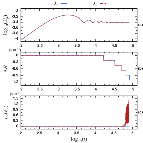
Figure 1: Newtonian Lagrange’s triangle solution. The upper panel (a)  shows the evolution of the Lyapunov indicator $\lambda^{*}_{p}(t,\delta X(0))$, the middle panel (b)  shows the conservation of the Hamiltonian $\Delta H$ and the lower panel (c)  shows the $L_{2}$ norm of the estimated errors. In every panel, the solid line denotes the solution obtained using the analytical Jacobian and the dashed line, the result provided by the numerical computation of the Jacobian (see Sec. III.1).

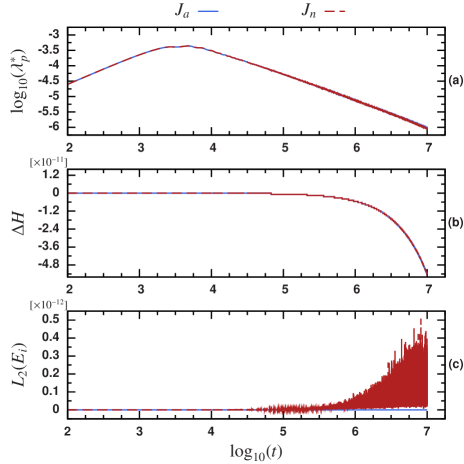
Figure 2: 1 PN Hénon Criss-cross solution. The upper panel (a) shows the evolution of the Lyapunov indicator $\lambda^{*}_{p}(t,\delta X(0))$, the middle panel (b)  shows the conservation of the Hamiltonian $\Delta H$ and the lower panel (c)  shows the $L_{2}$ norm of the estimated errors. In every panel, the solid line denotes the solution obtained using the analytical Jacobian and the dashed line, the result provided by the numerical computation of the Jacobian.

Fig. 1 (c)  illustrates the $L_{2}$ norm of the estimated errors for Lagrange’s triangle solution. By looking at the errors, the difference between the solution produced by $J_{n}$ and $J_{a}$ becomes clear. The numerical solution generates errors which are two orders of magnitude larger than the analytical Jacobian. However, even when using $J_{a}$, the accuracy is good, with errors below $1.5\times 10^{-8}$.

A second test was done for a stable system. Using the 1 PN equations of motion, we computed the Lyapunov indicator $\lambda^{*}_{p}$, the relative variation of the Hamiltonian $\Delta H$ and the $L_{2}$ norm of the estimated errors for the Hénon’s criss-cross solution Hen76 ; Moo93 ; Nau01 . We used initial parameters given by

$$\begin{array}[]{ll}\vec{x}_{1}(0)=1.07590\lambda^{2}\hat{x},&\vec{p}_{1}(0)=3^{-3/2}\cdot 0.19509\lambda^{-1}\hat{y},\\ \vec{x}_{2}(0)=-0.07095\lambda^{2}\hat{x},&\vec{p}_{2}(0)=-3^{-3/2}\cdot 1.23187\lambda^{-1}\hat{y},\\ \vec{x}_{3}(0)=-1.00496\lambda^{2}\hat{x},&\vec{p}_{3}(0)=3^{-3/2}\cdot 1.03678\lambda^{-1}\hat{y},\end{array}$$

where $\hat{x}$, $\hat{y}$ and $\hat{z}$ are the unitary basis vectors in Cartesian coordinates, and $\lambda$ is a scaling factor (for our simulation $\lambda=10$). Notice that for this test we used the parameters given in MooNau08 with the scaling factor $\lambda$, and doing a change of variables from initial velocity to initial momentum. Therefore, we are not including post-Newtonian corrections to the initial parameters. As in the previous case, $\lambda^{*}_{p}$ does not show significant differences when computed using $J_{a}$ or $J_{n}$ (see Fig. 2). The value of $\lambda^{*}_{p}$ decreases monotonically almost like a straight line; this is the characteristic behavior of a regular solution. The maximum relative difference in $\lambda^{*}_{p}$ using $J_{a}$ and $J_{n}$ is $8\times 10^{-6}$. The Hamiltonian is conserved with a maximum variation of $5\times 10^{-11}$. The $L_{2}$ norm of the estimated errors shows noisy errors using $J_{n}$ while $J_{a}$ exhibits a flat trend.

A third test was done with a known chaotic binary system. We used a chaotic eccentric configuration with mass ratio 3:2 and initial parameters:

$$\begin{array}[]{l}\vec{r}_{12}(0)=50\hat{x}\\ \vec{p}_{1}(0)=-\vec{p}_{2}(0)=0.0061644\hat{y}+0.003616\hat{z},\\ \vec{s}_{1}(0)=-0.43765200\hat{x}-0.11469240\hat{y}+0.29478960\hat{z},\\ \vec{s}_{2}(0)=-0.02443680\hat{x}+0.10324000\hat{y}-0.01104320\hat{z}.\end{array}$$ (26)

A similar system, with a different unit convention, was studied in HarBuo05 (Sec. IV-C1). Following HarBuo05 , we solved the equation of motion using up to 2 PN correction for the orbital part and leading order in the spin. As was emphasized in HarBuo05 , in this configuration, the two compact bodies are rather close to each other. In order to obtain an accurate physical description, it is necessary to include, for the orbital part, corrections higher than 2 PN and, for the spinning part, higher than the leading order. The 1 PN contribution to the Hamiltonian (22) during a close encounter of the bodies can reach 50%. At this point it is important to recall one of the conclusions of HarBuo05 . When using up to 2 PN Hamiltonian with leading order spin contributions, there is no evidence of chaotic systems for configurations which are physically valid to the PN order considered. Therefore, for comparison, this test was performed without using the stopping criteria $H_{1}^{\%}>10\%$.

The result of the third test is presented in Fig. 3. The system was evolved using the parameters given in (26), and for reference, a non-chaotic orbit with the same initial condition but with $\vec{s}_{1}(0)=\vec{0}$ was used. Fig. 3-(a) shows the Lyapunov indicator for the chaotic configuration (solid line) and the arithmetic mean computed for $t>10^{6}$. The estimated value of the Lyapunov indicator is $\langle\lambda_{p}^{*}\rangle=10^{-5}$ (dotted line) with a standard deviation of $1.3\times 10^{-6}$, corresponding to a relative variation of $13\%$. In contrast, the regular solution shows that $\lambda_{p}^{*}$ decreases almost monotonically after $t=10^{4}$. In both simulations, the Hamiltonian is numerically conserved below $10^{-8}$ (see Fig. 3-(b)), and the estimated errors are of order $10^{-6}$ for the chaotic solution and $10^{-10}$ for the regular solution. The main source for the errors, in the case of the chaotic solution, is the numerical calculation of the Jacobian matrix.

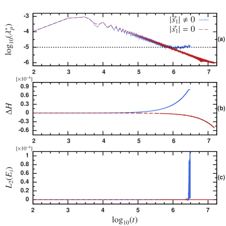
Figure 3: Spinning binaries with an eccentric orbit. Lyapunov function $\lambda^{*}_{p}(t,\delta X(0))$ (a), conservation of the Hamiltonian $\Delta H$ (b) and the $L_{2}$ norm of the estimated errors, for the system with initial parameters given by (26) (solid line) and the same configuration except for $\vec{s}_{1}(0)=\vec{0}$ (dashed line).

We performed, additional tests already presented in Sec. III-A of GalBru11 . A direct comparison with the results in GalBru11 does not showed significant differences in the results. For conciseness, we do not display the results of the tests.

III.2 Stability of hierarchical systems

Here, we consider the strong perturbation of a binary compact object system due to a third smaller compact object. As a basic configuration, we studied a Jacobian system with mass ratio 10:20:1. The inner binary system had initial apo-apsis ( i.e. maximum separation of a Keplerian orbit) $r_{b}(0)=130$ and eccentricity $e_{b}(0)=0$. Although there are methods in post-Newtonian dynamics to specify the initial parameters of a binary system with a given eccentricity (see e.g. HarBuo05 ; WalBruMue09 ; HusHanGon07 ; TicBruCam02 ; BerIyeWil06 ; PfeBroKid07 ), in this study the inner binary is strongly-perturbed by a third body. Therefore, it is necessary to account for additional effects. For simplicity, we set the initial parameters considering only the Newtonian dynamics of a non-perturbed binary, where the eccentricity refers to the Newtonian case. In this approach, we view the third compact body and the center of mass of the inner binary as a new binary (we will refer to it as the external binary). The bodies start from a configuration where the initial radial vector $\vec{r}_{12}$ is perpendicular to initial vector position $\vec{x}_{3}$ of the external body (see Fig. 4). We denote the inclination angle between the osculating orbital planes $\Pi_{\mathrm{in}}$ and $\Pi_{\mathrm{ext}}$ by $\iota$ (see Fig. 4). To be more specific, the initial position and momentum of each body is given by

$$\begin{array}[]{l}\vec{x}_{1}=\frac{m_{2}}{m_{b}}r_{b}\hat{x}-m_{3}r_{3}(\hat{y}\cos i+\hat{z}\sin i),\\ \vec{x}_{2}=\frac{m_{1}}{m_{b}}r_{b}\hat{x}-m_{3}r_{3}(\hat{y}\cos i+\hat{z}\sin i),\\ \vec{x}_{3}=m_{b}r_{3}(\hat{y}\cos i+\hat{z}\sin i),\\ \vec{p}_{1}=-p_{b}\hat{y}-\frac{m_{1}}{m_{b}}p_{3}\hat{x},\\ \vec{p}_{2}=p_{b}\hat{y}-\frac{m_{1}}{m_{b}}p_{3}\hat{x},\\ \vec{p}_{3}=p_{3}\hat{x},\end{array}$$ (27)

where $m_{b}:=m_{1}+m_{2}$, $p_{b}=m_{1}m_{2}\sqrt{(1-e_{b})/(m_{b}r_{b})}$ and $p_{3}=m_{b}m_{3}\sqrt{(1-e_{3})/r_{3}}$. Notice that we set the momentum in terms of the eccentricity and the apo-apsis. Therefore, a higher eccentricity given to the external binary implies a stronger perturbation of the inner binary.

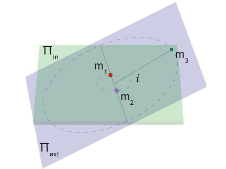
Figure 4: Hierarchical system (see GalBru11 ). Initial configuration of the inner and external binaries. The initial momentum of the third body is given by considering the external binary as a Newtonian binary. Shown are the osculating orbital planes $\Pi_{\mathrm{in}}$ and $\Pi_{\mathrm{ext}}$ for inner and external binary orbits. The two planes are inclined by an angle $\iota$.

The main goal of this study was to characterize the stability and chaos of a hierarchical system as function of the initial apo-apsis $r_{3}$, the eccentricity $e_{3}$ for the external binary and the inclination angle $\iota$ between the osculating orbital planes. We explored the influence of the post-Newtonian corrections.

III.2.1 Final state survey

An analysis of the asymptotic behavior of the system as function of three parameters $r_{3}$, $e_{3}$ and $\iota$ was performed. For a given osculating angle $\iota$, we produced a map which is a subset of the space of configurations $(r_{3},e_{3})$. We define three possible outcomes which characterize the asymptotic behavior of the system: the escape of one of the bodies, a strong interaction $H_{1}^{\%}>10\%$ and a system which remains stable up to $t_{f}=2\times 10^{7}$. We assign a color to each outcome in the map of initial configurations $(r_{3},e_{3})$: dark gray (color online) for an escape, white for a strong interaction and black for a stable configuration. Strictly speaking, the result is not a basin boundary map since the outcomes are not attractors in the phase space and the parameters $(r_{3},e_{3})$ are not coordinates of the phase space. However, Eqs. (27) gives the link between $(r_{3},e_{3})$ and the coordinates of the phase space. On the other hand, a system where one of the bodies escapes will be attracted to a hyper-plane in the phase space with one of the spatial coordinates at infinity; a strong interaction may become an escape or the merger of two of the bodies. A merger can be represented by a hyper-plane where two of the bodies share the same values of position and momentum. For a stable system, it is hard to define a single attractor because it can exhibit a different asymptotic behavior for $t>t_{f}$. For simplicity, we refer to the boundary between the various color in the map as basin boundary since it can capture some of the features of a basin boundary.

The choice of $t_{f}=2\times 10^{7}$ is motivated by the dynamics of a similar Jacobian system presented in GalBru11 . Including up to 2.5 PN terms, the inner binary arrives to the merger phase after $t_{\mathrm{mgr}}\approx 2.7\times 10^{7}$. The assumption is that if a conservative system remains stable until that time, then the corresponding radiative system will remain stable until the merger of the inner binary. We selected a shorter time (i.e., $t_{f}<t_{\mathrm{mgr}}$) due to computational costs. However, a set of numerical experiments for different values of $t_{f}$ suggest that a non-stable orbit is manifest before $t_{f}$.

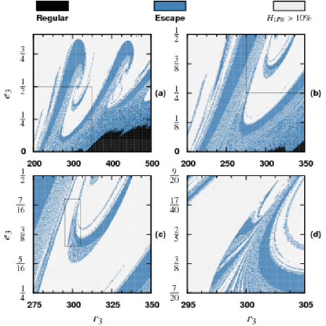
Figure 5: Fractal basin boundary (Newtonian). Result of the asymptotic behavior of initial conditions for the parameters $r_{3},e_{3}$ and $i=0$ for region $R_{0}$ (a), $R_{1}$ (b), $R_{2}$ (c) and $R_{3}$ (d). The black points denote stable orbits, dark gray points (blue color online) are escapes of the lighter body and white points denote a strong interaction of two of the bodies.

We explored the parameter space $r_{3},e_{3}$ using 4 regions defined by

$$\begin{array}[]{lll}R_{0}:[200,500]\times[0,1],&\Delta r_{3}=1,&\Delta e_{3}=0.0025;\\ R_{1}:[200,350]\times[0,0.5],&\Delta r_{3}=0.5,&\Delta e_{3}=0.00125;\\ R_{2}:[275,350]\times[0.25,0.5],&\Delta r_{3}=0.25,&\Delta e_{3}=0.000625;\\ R_{3}:[295,305]\times[0.35,0.45],&\Delta r_{3}=0.05,&\Delta e_{3}=0.00025.\end{array}$$

The domain of each region is the Cartesian product and its resolution is denoted by $\Delta r_{3},\Delta e_{3}$. Each map was done computing $300\times 400$ orbits except for region $R_{3}$ that contains $200\times 400$ orbits. Fig. 5 shows the result for a Newtonian simulation and osculating angle $i=0$. Notice that $R_{3}\subset R_{2}\subset R_{1}\subset R_{0}$, i.e. each $R_{i}$ is a magnification of the region $R_{i-1}$ (in the figure, the sub-regions are indicated by rectangles). Fig. 5 shows the characteristic behavior of a fractal set; every magnification reveals a more complex structure from which it is possible to distinguish some degree of self-similarity. Table 1 summarizes the quantitative results for the basin boundary. Notice that the box-dimension reflects the fact that the sets are not perfectly self-similar. We choose $R_{1}$ and $R_{2}$ to perform additional simulations.

Table 1: Newtonian orbits. Here $\mathrm{d}_{\mathrm{box}}$ is the box dimension of the basin boundaries presented in Fig. 5, the columns ‘Regular’, ‘Escape’ and ‘$H_{1\mathrm{PN}}>10\%$’ denote the percentage of simulation that have the corresponding final state.

Region	$\mathrm{d}_{\mathrm{box}}$	Regular	Escape	$H_{1\mathrm{PN}}>10\%$
$R_{0}$	$1.76\pm 0.015$	8.2%	32.4%	59.4%
$R_{1}$	$1.84\pm 0.013$	1.0%	41.3%	57.7%
$R_{2}$	$1.77\pm 0.015$	0.0%	24.7%	75.3%
$R_{3}$	$1.74\pm 0.007$	0.0%	27.2%	72.8%

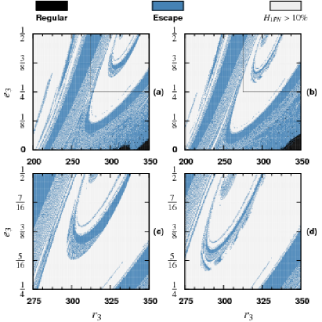
Figure 6: Fractal basin boundary (Newtonian and 1 PN). Comparison of regions $R_{1}$ and $R_{2}$ for Newtonian and 1 PN orbits. Panels (a)  and (b)  show $R_{1}$ for Newtonian and 1 PN respectively. Similarly, panels (c) and (d) show $R_{2}$ for Newtonian and 1 PN, respectively.

A comparison using Newtonian and 1 PN orbits for regions $R_{1}$ and $R_{2}$ is presented in Fig. 6. There is a clear difference in the set of stable orbits. In the Newtonian case, there are two disjoint sets where the 1 PN system exhibits a single set (compare the black point in panels (a)  and (b)  of Fig. 6). The magnification $R_{2}$ shows differences in the escape and strong interaction zones. The 1 PN case exhibits slightly different substructures (see panels (c) and (d) of Fig. 6). Our comparison includes a set of simulations for leading order spinning 1 PN particles. We employed maximally spinning particles $\chi_{a}=1$ and $\theta_{a}=0,\phi_{a}=0$ except by $\theta_{1}=\pi/2,\theta_{2}=2\pi/2$ (see Eq. (4)). Therefore, the initial spin of the particles (configuration-a) is given by

$$\begin{array}[]{l}\vec{s}_{1}=m_{1}^{2}\hat{x},\\ \vec{s}_{2}=-m_{2}^{2}\hat{x},\\ \vec{s}_{3}=m_{3}^{2}\hat{z},\end{array}$$ (28)

Opposite to the non-spinning case, the orbits for our configuration of spinning particles are not coplanar. However, the change in the final states is negligible, the resulting map is almost indistinguishable to the 1 PN case (for brevity, we do not display the basin boundaries which are similar to panels (b) and (d) of Fig. 6). The quantitative analysis of the six basin boundaries under comparison is displayed in Table 2. The difference on the substructures between the Newtonian case and the 1 PN case is reflected by the box-dimension (smaller value for the 1 PN case). In the region $R_{1}$, there is a small change in the distribution of ‘Regular’, ‘Escape’ and strong interactions between Newtonian and 1 PN. Nevertheless, in region $R_{2}$ there are noticeable differences in the percentages of ‘Escape’ and strong interactions. The similarity between the spinning and the non-spinning 1 PN case appears for the dimension and the distribution of the three outcomes (with minor differences in the percentages).

Table 2: Comparison of Newtonian, 1 PN, radiative 1 PN and leading order spinning 1 PN orbits. Here column $\mathrm{PN}$ takes value 0 for Newtonian, 0+1 for 1 PN and 0+1+2.5 for radiative 1 PN. The column $\mathrm{Sp}$ takes value 0 for non-spinning particles and 1 for the spinning ones. The meaning of the remaining columns is similar to Table 1. See the text for details about the parameters of the spinning case (Fig. 6 and 7 shows the non-spinning cases).

	$\mathrm{PN}$	$\mathrm{Sp}$	$\mathrm{d}_{\mathrm{box}}$	Regular	Escape	$H_{1\mathrm{PN}}>10\%$
$R_{1}$	0	0	$1.84\pm 0.013$	1.0%	41.3%	57.7%
	0+1	0	$1.81\pm 0.014$	1.4%	40.3%	58.3%
	0+1	1	$1.81\pm 0.014$	1.2%	40.7%	58.1%
	0+1+2.5	0	$1.81\pm 0.014$	1.7%	40.0%	58.3%
$R_{2}$	0	0	$1.77\pm 0.015$	0.0%	24.7%	75.3%
	0+1	0	$1.74\pm 0.015$	0.0%	18.0%	82.0%
	0+1	1	$1.74\pm 0.015$	0.0%	18.1%	81.9%

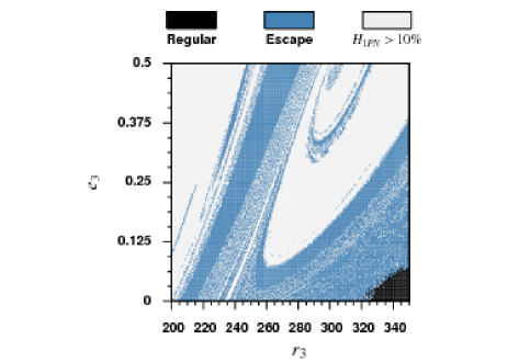
Figure 7: Basin boundary of region $R_{1}$. The dynamic includes (0+1+2.5) PN terms.

In order to investigate the influence of the gravitational radiation, we performed an evolution which contains the 2.5 PN terms. The inclusion of PN terms is computationally expensive. Therefore, we used a radiative 1 PN Hamiltonian (i.e., we include the Newtonian, 1 PN and 2.5 PN terms in (2)). For similar configurations, the difference in the dynamics between the full 2.5 PN system and the radiative 1 PN is relatively small GalBru11 . Fig. 7 shows the fractal basin boundary and Table 2 the corresponding quantitative measures. The radiative term does not seem to produce a significant change in respect of the inclusion of 1 PN terms (compare Fig. 7 with Fig. 6-(b)). Particularly, the box-dimension of the boundary is the same, and there is only a small difference in the distribution of the percentages of escape and strong interactions.

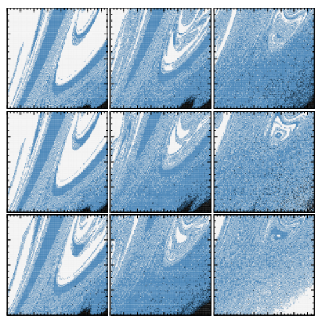
Figure 8: Fractal basin boundary of region $R_{1}$ as function of the osculating angle $\iota$ (Newtonian). The meaning of the color is the same as in previous plots (see e.g. Fig. 6). From the top to the bottom and from the left to the right $\iota$ takes the values $0,\pi/16,\pi/8,3\pi/16,\pi/4,5\pi/16,3\pi/8,7\pi/16,\pi/2$.

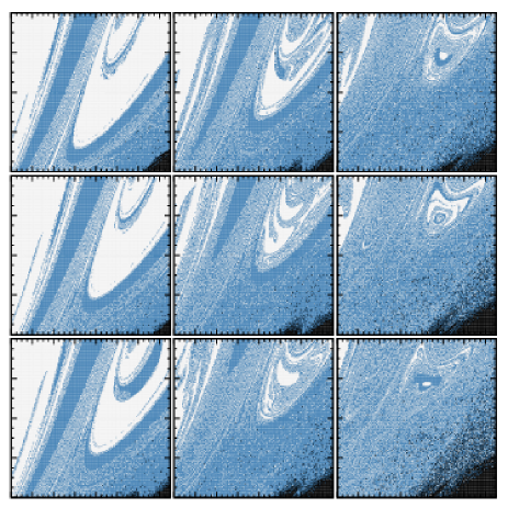
Figure 9: Fractal basin boundary of region $R_{1}$ as function of the osculating angle $\iota$ (1 PN). The meaning of the color is the same as in previous plots (see e.g. Fig. 6). From the top to the bottom and from the left to the right $\iota$ takes the values $0,\pi/16,\pi/8,3\pi/16,\pi/4,5\pi/16,3\pi/8,7\pi/16,\pi/2$.

The osculating angle $\iota$ has a strong influence in the region of the initial parameters $R_{1}$. For the Newtonian case, we produced a set of eight additional maps for region $R_{1}$ where the osculating angle takes the values $\iota=n\pi/16$, $n\in\{1,2,\dots,8\}$. The results, including the case $\iota=0$, are presented in Fig. 8. An analogous set of simulations was produced using the 1 PN equation of motion. Fig. 9 shows the corresponding basin boundaries. Table 3 shows the quantitative results for both sets. Notice that for $i>\pi/4$ the percentage of stable points considerably increases for the 1 PN case in respect of the Newtonian. The box-dimension in both cases has a growing-oscillatory behavior. Fig. 10 shows the results for the uncertainty exponent $\alpha$. A relatively simple function $\alpha_{\mathrm{fit}}(\iota)=a_{i}\iota+b_{i}+c_{i}\sin\varphi_{i}\iota$ fits the data. The fit parameters are

$$\begin{array}[]{ll}a_{\mathrm{N}}=-0.059\pm 0.0088,&a_{1\mathrm{PN}}=-0.097\pm 0.0065,\\ b_{\mathrm{N}}=0.144\pm 0.0079,&b_{1\mathrm{PN}}=0.183\pm 0.0059,\\ c_{\mathrm{N}}=0.026\pm 0.0062,&c_{1\mathrm{PN}}=0.018\pm 0.0047,\\ \varphi_{\mathrm{N}}=7.1\pm 0.27,&\varphi_{1\mathrm{PN}}=6.3\pm 0.27.\end{array}$$ (29)

The slope of the linear part of the 1 PN is 1.6 times larger than the Newtonian one. However, the oscillatory part is nearly 0.7 times the 1 PN value for the Newtonian case. This result shows that the chaotic properties of this hierarchical configuration increases in both cases, reaching the maximum at $\iota=\pi/2$. From the basin boundary figures, we can notice an increasing number of unsafe points. There is an evident difference for $\iota=\pi/2$ between the Newtonian and 1 PN basin boundary (comparing the bottom-right panel of Figs. 8 and 9). We analyze this particular case in the next section.

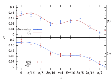
Figure 10: Uncertainty exponent $\alpha$ as function of the osculating angle $\iota$ for the region $R_{1}$. The upper panel (a) shows the result for the Newtonian case, the solid line is the fitting function $\alpha^{\mathrm{N}}_{\mathrm{fit}}(\iota)=a_{\mathrm{N}}\iota+b_{\mathrm{N}}+c_{\mathrm{N}}\sin\varphi_{\mathrm{N}}\iota$. The lower panel (b) shows the corresponding result for the 1 PN simulations, where the solid line is $\alpha^{\mathrm{PN}}_{\mathrm{fit}}(\iota)=a_{\mathrm{PN}}\iota+b_{\mathrm{PN}}+c_{\mathrm{PN}}\sin\varphi_{\mathrm{PN}}\iota$. The fitting parameters are given in Eq. (29).

Table 3: Measures of the basin boundaries of Figs. 8 and 9. The osculating angle is denoted by $\iota$. The meaning of the remaining columns is similar to Table 2.

	Newtonian				1 PN
$\iota$	$\mathrm{d}_{\mathrm{box}}$	Regular	Escape	$H_{1\mathrm{PN}}>10\%$	$\mathrm{d}_{\mathrm{box}}$	Regular	Escape	$H_{1\mathrm{PN}}>10\%$
0	$1.84\pm 0.013$	1.0%	41.3%	57.7%	$1.81\pm 0.014$	1.4%	40.3%	58.3%
$\pi/16$	$1.85\pm 0.013$	1.0%	43.0%	56.0%	$1.82\pm 0.014$	0.7%	41.6%	57.7%
$\pi/8$	$1.88\pm 0.013$	1.1%	49.2%	49.7%	$1.84\pm 0.013$	0.9%	48.2%	50.9%
$3\pi/16$	$1.92\pm 0.012$	1.9%	62.3%	35.8%	$1.90\pm 0.012$	1.5%	58.0%	40.5%
$\pi/4$	$1.91\pm 0.012$	2.7%	67.9%	29.4%	$1.91\pm 0.012$	2.2%	64.2%	33.6%
$5\pi/16$	$1.90\pm 0.012$	2.7%	74.3%	23.0%	$1.91\pm 0.012$	3.2%	67.9%	28.9%
$3\pi/8$	$1.89\pm 0.013$	2.2%	77.5%	20.3%	$1.92\pm 0.012$	4.3%	70.8%	24.9%
$7\pi/16$	$1.94\pm 0.012$	1.5%	73.9%	24.6%	$1.94\pm 0.012$	6.1%	69.3%	24.6%
$\pi/2$	$1.98\pm 0.011$	0.1%	57.1%	42.8%	$1.97\pm 0.011$	9.3%	67.4%	23.3%

III.2.2 Analysis of orbits

We used the basin boundaries as a guide for a detailed study of specific orbits. Given the region $R_{1}$, an osculating angle $\iota$, two different basin boundaries $\Omega(r_{3},e_{3})$ and $\Omega^{*}(r_{3},e_{3})$, it is possible to produce a new map $D$ that shows the differences between $\Omega(r_{3},e_{3})$ and $\Omega^{*}(r_{3},e_{3})$. We constructed the map as follows; $D(r_{3},e_{3})$ takes value 1 if $\Omega(r_{3},e_{3})=\Omega^{*}(r^{*}_{3},e^{*}_{3})$ in a neighborhood of $(r_{3},e_{3})$ of size at least $6\mathrm{d}r_{3}\times 6\mathrm{d}e_{3}$, i.e., for $r^{*}_{3}=r_{3}+i\mathrm{d}r_{3}$, $e^{*}_{3}=e_{3}+i\mathrm{d}e_{3}$ and $i\in\{-3,-2,\dots,3\}$. If the previous condition is not satisfied, then the $D(r_{3},e_{3})$ is set to 0. $D(r_{3},e_{3})$ provides a way for identifying zones where the two basin boundaries differed in a relatively large region. From the analysis of this map and the basin boundaries, we explored several initial parameters where we compared the orbits for different configurations of the PN equations of motion. In the following, we describe 5 representative comparisons.

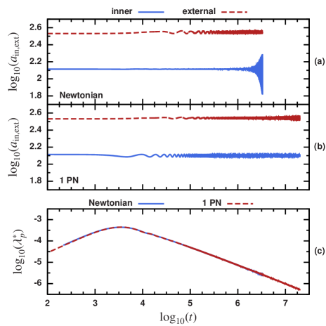
Figure 11: Semi-major axis and Lyapunov function for initial parameters $\iota=\pi/2,r_{3}=340,e_{3}=0$. The upper panel (a) shows the semi-major axis $a$ of the inner and external binaries as function of time for the Newtonian case. The middle panel (b) is similar to (a) but for the 1 PN case. The lower panel (c)  shows the evolution of the Lyapunov indicator for both cases. Notice that the quantities are given in $log_{10}$ scales.

For the region $R_{1}$ and $\iota=\pi/2$ there is a clear difference between the Newtonian and 1 PN evolution (i.e., the difference between the bottom-right panel of Figs. 8 and 9). The bottom-right zone of parameters leads to a different outcome. In the Newtonian case, the simulation with parameters $e_{3}<(r_{3}-310)/320$ ends when $H_{1\mathrm{PN}}>10\%$. However, for the same set of parameters the 1 PN case remains stable. For the Newtonian case, there is a fast growth on the eccentricity of the inner binary induced by the external body (see Fig. 11-(a)). This effect is produced by a resonance between the orbital dynamic of the inner and external binary (see Mar08 for a detailed description). For the 1 PN case the orbits remain stable during the simulation (see Fig. 11-(b)). In both cases, the evolution of the Lyapunov indicator does not showed evidence of exponential growth behavior (see Fig. 11-(c)). Notice that in the Newtonian case, the strong interaction is between the components of the inner binary. The behavior of the Lyapunov function suggests that the strong interaction between the heavy components of the system does not follow chaotic trajectories.

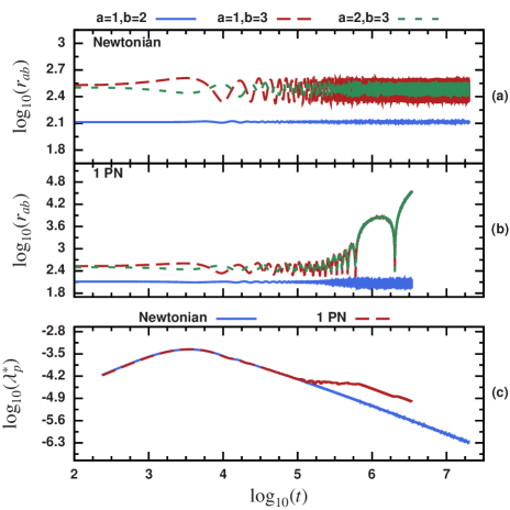
Figure 12: Relative separation and Lyapunov function for initial parameters $\iota=0,r_{3}=320,e_{3}=0$. The upper panel (a) shows the relative separation $r_{ab}$ between particles as function of time for the Newtonian case. The middle panel (b) is similar to (a)  but for the 1 PN case. The lower panel (c)  shows the evolution of the Lyapunov indicator for both cases.

For the region $R_{1}$ and $\iota=0$, there is a significant difference between the Newtonian and the 1 PN basin boundaries for stable orbits (i.e., the black dots in panels (a)  and (b)  of Fig. 6). The Newtonian configuration remains stable without noticeable instability. On the other hand, the coupling between the orbits in the 1 PN case results in the escape of the third body (see panels (a)  and (b) of Fig. 12). The Lyapunov function shows for 1 PN dynamics the characteristic behavior of escape orbits. During a close encounter between the lighter body and one of the heavy components of the inner binary, the difference vector has an exponential growth which is followed by a regular behavior. The regular behavior is expected for an uncoupled binary-single body system (see the kink in the Lyapunov function of Fig. 12-(c)). The exponential growth for the difference vector is an indication of sensitivity to initial conditions. In general, the resulting escape orbit is chaotic; a small change in the initial condition produces a significant change in the escape direction.

A comparison between 1 PN and 2 PN dynamics showed that almost identical orbits are produced by an evolution where the lighter body has a quick encounter with the inner binary which is followed by an escape or a strong interaction. Fig. 13 displays a comparison between the Newtonian, 1 PN and 2 PN evolutions for 11 nearby configurations. The initial parameters are $\iota=0$ and $e_{3}=0.1$ with $r_{3}\in\{269.95,269.96,\dots,270.05\}$. The relative change in the initial separation $r_{3}$ between the configurations is $\sim~{}0.004\%$. The Newtonian evolution (Fig. 13-(a)), exhibits a chaotic behavior. Every simulation ends with the escape of the lighter body. There are significant differences in the trajectories. On the other hand, the 1 PN and 2 PN evolutions (panels (b) and (c) of Fig. 13) produce a quick escape which are similar for each initial condition. The maximum final difference between the orbits is $1.3\%$ for the 1 PN case and $1.5\%$ for the 2 PN simulations. Moreover, the final difference between the 1 PN and 2 PN reference evolution $r_{3}=270$ is $6\%$.

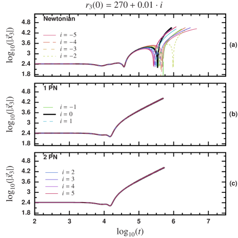
Figure 13: Evolution of the coordinate position $|\vec{x}_{3}|$ for 11 nearby configurations. Initial parameters $\iota=0,e_{3}=0.1$ and $r_{3}\in\{269.95,269.96,\dots,270.05\}$. The upper panel (a) shows Newtonian case, the middle panel (b) shows the 1 PN evolution and the lower panel (c)  the 2 PN case.

However, for successive encounters the evolution is significantly different. Fig. 14 shows the resulted orbits for initial parameters $\iota=0,r_{3}=240,e_{3}=0$. For these initial parameters, the resulting outcome is the escape of the lighter body. Nevertheless, in the 1 PN evolution there is an ejection of the lighter body before the final escape. In contrast, the ejection is not present in the 2 PN orbit (compare panels (a)  and (b) of Fig. 14). There is a significant difference in the evolution of the Lyapunov function. For the 1 PN case, there is a double kink which corresponds to the close encounters before and after the ejection. Nevertheless, the 2 PN evolution presents a single long kink (see Fig. 14-(c)).

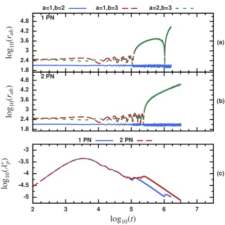
Figure 14: Relative separation and Lyapunov function for initial parameters $\iota=0,r_{3}=280,e_{3}=0$. The upper panel (a) shows the relative separation $r_{ab}$ between particles as function of time for the 1 PN case. The middle panel (b)  is similar to (a)  but for the 2 PN case. The lower panel (c)  shows the evolution of the Lyapunov indicator for both cases.

Fig. 15 shows a comparison between the Newtonian, 1 PN and 2 PN evolutions for 11 nearby configurations. The initial parameters are $\iota=0$ and $e_{3}=0$ with $r_{3}\in\{279.95,279.96,\dots,280.05\}$. Similarly to the case presented in Fig. 13, the relative change in the initial separation $r_{3}$ between the configurations is $\sim 0.004\%$. The set of configurations includes the solution presented in Fig. 14 $r_{3}=280$. The evolutions exhibit sensitive dependence on initial conditions. In the three cases, Newtonian, 1 PN and 2 PN, relatively nearby initial parameters produce a significant change in the orbits. Moreover, the inclusion of PN corrections produced a noticeable change in the trajectories.

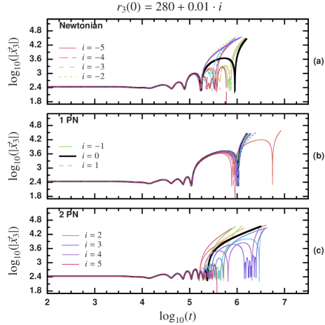
Figure 15: Evolution of the coordinate position $|\vec{x}_{3}|$ for 11 nearby configurations. Initial parameters $\iota=0,e_{3}=0$ and $r_{3}\in\{279.95,279.96,\dots,280.05\}$. The upper panel (a) shows Newtonian case, the middle panel (b) shows the 1 PN evolution and the lower panel (c) the 2 PN case. The bold-black line is the reference solution presented in Fig. 14.

For the parameters that we have studied, the inclusion of spin correction has a small influence in the final outcome. However, like in the 2 PN case, for some of the initial parameters, the evolution is completely different. For the initial parameters $\iota=0,r_{3}=320$ and $e_{3}=0.39$, the 1 PN orbit ends with the strong interaction between particles 1 and 3 (see Fig. 16-(a)). In contrast, the spinning leading order 1 PN for the spin configuration-a (28) results with the escape of particle 3 (see Fig. 16-(b)). For the escaping orbit, the evolution produces a Lyapunov function which after $t=10^{5}$ decreases linearly. The spinning case shows initially the same trend. However, the strong interaction produces a short kink at the end of the evolution (see Fig. 16-(c)).

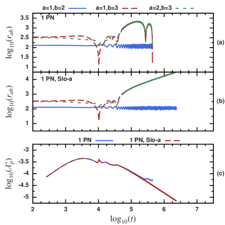
Figure 16: Relative separation and Lyapunov function for initial parameters $\iota=0,r_{3}=320,e_{3}=0.39$. The upper panel (a) shows the relative separation $r_{ab}$ between particles as function of time for the 1 PN case. The middle panel (b) is similar to (a)  but for the leading order spinning 1 PN configuration-a (initial spin given by (28)). The lower panel (c)  shows the evolution of the Lyapunov indicator for both cases.

We explored a different set of spin parameters. Here we present one of the results of configuration-b given by

$$\begin{array}[]{l}\vec{s}_{1}=m_{1}^{2}\hat{x},\\ \vec{s}_{2}=m_{2}^{2}\hat{x},\\ \vec{s}_{3}=m_{3}^{2}\hat{y}.\end{array}$$ (30)

Fig. 17 shows the result for the initial parameters $\iota=\pi/4,r_{3}=242,e_{3}=0.2$ for the 1 PN and spinning leading order 1 PN cases. In this evolution, the non-spinning case results in the escape of particle 3. For the spinning particles, the result is the strong interaction between particles 1 and 3. The Lyapunov function shows the characteristic exponential growth of the difference vector during the close interaction.

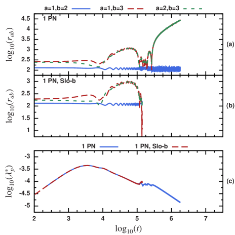
Figure 17: Relative separation and Lyapunov function for initial parameters $\iota=\pi/4,r_{3}=242,e_{3}=0.2$. The upper panel (a) shows the relative separation $r_{ab}$ between particles as function of time for the 1 PN case. The middle panel (b) is similar to (a)  but for the spinning leading order 1 PN configuration-b (initial spin given by (30)). The lower panel (c)  shows the evolution of the Lyapunov indicator for both cases.

Table 4: Evolution of the eccentricity of the inner binary $e_{b}$. Here we refer to the orbits in terms of the figure given in the column ‘Fig.’, $e_{b}(0)$ is the initial eccentricity of the inner binary and $e_{b}(t_{f})$, the final eccentricity computed before the corresponding simulation finish. $\langle e_{b}\rangle$ and $\sigma(e_{b})$ are the arithmetic mean and standard deviation of $e_{b}$ respectively. The column ‘FS’ refers to the final state of the evolution.

#	Fig.	$e_{b}(0)$	$e_{b}(t_{f})$	$\langle e_{b}\rangle$	$\sigma(e_{b})$	FS
1	11-(a)	0.004	0.493	0.112	0.1453	$H_{1\mathrm{PN}}>10\%$
2	11-(b)	0.040	0.040	0.039	0.0003	Regular
3	12-(a)	0.021	0.030	0.025	0.0047	Regular
4	12-(b)	0.036	0.281	0.252	0.0556	Escape
5	14-(a)	0.042	0.140	0.117	0.0225	Escape
6	14-(b)	0.062	0.104	0.104	0.0074	Escape
7	16-(a)	0.030	0.155	0.185	0.0332	$H_{1\mathrm{PN}}>10\%$
8	16-(b)	0.137	0.184	0.184	0.0049	Escape
9	17-(a)	0.095	0.237	0.225	0.0343	Escape
10	17-(b)	0.024	0.004	0.071	0.0299	$H_{1\mathrm{PN}}>10\%$

Table 4 shows the evolution of the eccentricity of the inner binary $e_{b}$. The eccentricity is computed by calculating numerically the value of the apo-apsis and peri-apsis of the inner binary i.e., computing a sequence of local maxima and minima of $r_{12}$. The eccentricity is given by

$$e_{b}=\frac{r_{\mathrm{ap}}-r_{\mathrm{per}}}{r_{\mathrm{ap}}+r_{\mathrm{per}}}.$$ (31)

Notice that the initial value of $e_{b}$ in every case is relatively small but not zero due to the perturbation of the third body. However, the final value of the eccentricity depends on the final state of the evolution. For regular orbits, the change is relatively small (see the standard deviation of rows 2 and 3 in Table 4). On the other hand, the final eccentricity of the escaping orbits is relatively large during the whole evolution (compare the final eccentricity and the arithmetic mean of the corresponding rows). The orbit with resonance exhibits the largest increment in eccentricity. The final value before the evolution stops is close to 0.5. For PN evolutions, we did not find evolutions with this kind of resonance. However, a different set of parameters may lead to similar behavior. For a strong interaction between two of the bodies, the resulting final eccentricity is not meaningful since there are two possible outcomes in the full evolution scenario. One possibility is an ejection or escape of the lighter body leading to a increment in the eccentricity of the inner binary similar to the cases presented. The other possibility is a successive merger of the three bodies.

IV Discussion

We performed a numerical study of stability and chaos of a hierarchical three compact object configuration. The configuration is composed by a binary system which is perturbed by a third, lighter body positioned initially far away from the binary. For a given inner binary, we explored the influence of the third body taking as free parameters the angle of the osculating orbital planes, the initial apo-apsis and eccentricity of the third body. Using the basin boundary method, a total of 2,960,000 simulations were analyzed. From the total, 47.3% corresponded to Newtonian evolutions, 40.54% to (0+1) PN simulations, 4.05% to (0+1+2.5) PN evolutions and 8.11% are simulations of spinning particles including leading order in spin and 1 PN terms in the orbital part.

A total of twenty-five basin boundary maps were produced. The basin boundaries exhibit the characteristics of fractal sets: some degree of self-similarity and an increasing complexity under magnification. Fractal basin boundaries are an indicator of chaos in dynamical systems. By measuring the fractal dimension of the basin boundaries it is possible to determine the uncertainty exponent $\alpha$. The property of the exponent is that for $\alpha\approx 0$ the dynamical system is chaotic and for $\alpha=1$ the system is regular. The values of $\alpha$ for the fractal basin boundaries considered here are between 0.02 and 0.26. The 1 PN set of data produces an exponent slightly larger than the Newtonian case (the maximum difference is 1.6%). On the other hand, the osculating angle $\iota$ has a strong influence in the uncertainty exponent. The exponent decreases as a linear oscillatory function in the range $[0,\pi/2]$. The difference between the planar case ($\iota=0$) and the case where the third body starts from a direction perpendicular to the orbital plane of the inner binary ($\iota=\pi/2$) is 7.1% for the Newtonian simulations and 8.1% for the 1 PN case.

In addition to the uncertainty exponent, we quantified the percentage of stable orbits, escapes and strong interactions. The configurations selected contain between 0% and 9.3% of stable orbits. The distribution of escapes are between 40.3% and 77.6%. The strong interactions oscillate between 20.3% and 82%. A remarkable case was found at $\iota=\pi/2$ where the Newtonian simulation presents a resonance which drops the number of stable orbits to 0.1%. Opposite to the Newtonian case, a dynamic including 1 PN or higher corrections eliminates the resonance. The number of stable orbits increases to 9.3%. The presence of resonances in the three-body problem is fundamental for understanding the chaotic properties of the system, see e.g. Mar08 ; ValKar06 ; SetMut11 and references therein.

By looking at specific orbits, it is possible to notice some of the different couplings between the inner and external binaries. For most of the orbits, the 1 PN terms have the strongest effect on the dynamics. The inclusion of the spinning particles or 2 PN corrections produces small differences in the orbits when the lighter body has a quick encounter with the inner binary which is followed by an escape or a strong interaction. In that cases the orbits are essentially identical. However, the coupling of the orbits for some of the configurations can produce a significant change in the final outcome. We presented five representative examples.

The spin can produce a significant change in the orbits producing precession of the orbital planes. However, the change on the dynamics is not strong enough to modify the final outcome. On the other hand, gravitational radiation, in general, produces a small change in the energy to be significant in the short time scale of the evolution. Similarly to the spinning case, gravitational radiation has a small effect in the asymptotic behavior.

Considering the scenario of a binary system in a galactic core or a region with high density of compact objects, we expect to have the following results. Between a 40% and 70% probability that the lighter body escapes the system depending on the relative orbital planes. The remanent binary may result in eccentricities between 0.1 and 0.2. Between 23% and 58% of the bodies may lead to a merger with one of the components of the inner binary; contributing to the growth of the compact objects. The probability of finding a body in a stable orbit is between 1% and 10%, producing a perturbation which leads to small eccentricities of the inner binary of around 0.03. Nevertheless, the combined effect of many bodies of comparable size can significantly change the results.

More general statements about the chaotic behavior of three compact bodies are possible but require an extensive parameter study. Other configurations include, for example, a characterization of the stability and chaos based on the mass ratios, inner binary separation, magnitude and direction of the spin or initial eccentricity of the inner binary. We consider this a topic for future study.

- (1) K. Gultekin, M. C. Miller, and D. P. Hamilton, AIP Conf. Proc. 686, 135 (2003), arXiv:astro-ph/0306204
- (2) K. Gultekin, M. C. Miller, and D. P. Hamilton, The Astrophysical Journal 616, 221 (2004), arXiv:astro-ph/0402532
- (3) K. Gultekin, M. C. Miller, and D. P. Hamilton, The Astrophysical Journal 640, 156 (2006), arXiv:astro-ph/0509885
- (4) M. Iwasawa, Y. Funato, and J. Makino, The Astrophysical Journal 651, 1059 (2006), arXiv:astro-ph/0511391
- (5) L. Hoffman and A. Loeb, Mon. Not. R. Astron. Soc. 377, 957 (2007), arXiv:astro-ph/0612517
- (6) L. Hoffman and A. Loeb, The Astrophysical Journal 638, L75 (2006), arXiv:astro-ph/0511242
- (7) A. Gualandris, S. Portegies Zwart, and M. S. Sipior, Mon. Not. R. Astron. Soc. 363, 223 (Oct. 2005), arXiv:astro-ph/0507365
- (8) S. Mikkola, Mon. Not. R. Astron. Soc. 203, 1107 (Jun. 1983), http://adsabs.harvard.edu/abs/1983MNRAS.203.1107M
- (9) S. Mikkola, Mon. Not. R. Astron. Soc. 207, 115 (Mar. 1984), http://adsabs.harvard.edu/abs/1984MNRAS.207..115M
- (10) M. C. Miller and D. P. Hamilton, The Astrophysical Journal 576, 894 (2002), arXiv:astro-ph/0202298
- (11) P. Heinämäki, A&A 371, 795 (Jun. 2001)
- (12) M. Valtonen and S. Mikkola, Annu. Rev. Astron. Astrophys. 29, 9 (1991)
- (13) M. Milosavljević and D. Merritt, AIP Conference Proceedings 686, 201 (2003), http://link.aip.org/link/?APC/686/201/1
- (14) M. J. Valtonen, S. Mikkola, P. Heinamaki, and H. Valtonen, Astrophys. J. Suppl. 95, 69 (Nov. 1994)
- (15) P. Amaro-Seoane and M. Dewi Freitag, ArXiv e-prints(2010), arXiv:1009.1870 [astro-ph.CO]
- (16) J. Levin and H. Contreras, ArXiv e-prints(Sep. 2010), arXiv:1009.2533 [gr-qc]
- (17) N. Seto and T. Muto, Phys. Rev. D 81, 103004 (May 2010)
- (18) N. Seto and T. Muto, ArXiv e-prints(2011), arXiv:1105.1845 [astro-ph.CO]
- (19) N. Stone and A. Loeb, ArXiv e-prints(2010), arXiv:1004.4833 [astro-ph.CO]%%CITATION = 1004.4833;%%
- (20) X. Chen, A. Sesana, P. Madau, and F. K. Liu, Astrophys. J 729, 13 (2011), http://stacks.iop.org/0004-637X/729/i=1/a=13
- (21) M. J. Valtonen and H. Karttunen, The three-body problem (Cambridge University Press, New York, 2006) ISBN 0-521-85224-2 (hardcover)
- (22) J. Levin, Phys. Rev. Lett. 84, 3515 (Apr 2000), http://link.aps.org/doi/10.1103/PhysRevLett.84.3515
- (23) N. J. Cornish and J. Levin, Phys. Rev. D 68, 024004 (Jul. 2003)
- (24) J. D. Barrow and J. Levin(Mar. 2003), arXiv:nlin/0303070 [nlin.CD]
- (25) J. Levin, Phys. Rev. D 74, 124027 (Dec. 2006), arXiv:gr-qc/0612003
- (26) A. Gopakumar and C. Königsdörffer, Phys. Rev. D 72, 121501 (Dec. 2005), arXiv:gr-qc/0511009
- (27) W. Han, Gen. Rel. Grav. 40, 1831 (Sep. 2008), arXiv:1006.2229 [gr-qc]
- (28) J. D. Schnittman and F. A. Rasio, Phys. Rev. Lett 87, 121101 (Sep. 2001), arXiv:gr-qc/0107082
- (29) T. Damour, P. Jaranowski, and G. Schäfer, Phys. Rev. D 77, 064032 (2008), arXiv:0711.1048 [gr-qc]
- (30) J. Steinhoff, S. Hergt, and G. Schäfer, Phys. Rev. D 77, 081501 (Apr 2008), arXiv:0712.1716 [gr-qc]
- (31) J. Hartung and J. Steinhoff, Phys. Rev. D 83, 044008 (Feb 2011), arXiv:1011.1179 [gr-qc]
- (32) C. Moore, Phys. Rev. Lett. 70, 3675 (Jun 1993)
- (33) T. Imai, T. Chiba, and H. Asada, Phys. Rev. Lett. 98, 201102 (May 2007)
- (34) C. O. Lousto and H. Nakano, Class. Quantum Grav. 25, 195019 (2008), arXiv:0710.5542 [gr-qc]
- (35) K. Yamada and H. Asada, Phys. Rev. D 82, 104019 (Nov 2010), arXiv:1010.2284 [gr-qc]
- (36) K. Yamada and H. Asada, ArXiv e-prints(2010), arXiv:1011.2007 [gr-qc]
- (37) T. Ichita, K. Yamada, and H. Asada, ArXiv e-prints(2010), arXiv:1011.3886 [gr-qc]
- (38) J. D. Schnittman, ArXiv e-prints(2010), arXiv:1006.0182 [astro-ph.HE]
- (39) P. Galaviz and B. Brügmann, Phys. Rev. D 83, 084013 (Apr 2011)
- (40) M. Campanelli, C. O. Lousto, and Y. Zlochower, Phys. Rev. D77, 101501(R) (2008), arXiv:0710.0879 [gr-qc]
- (41) C. O. Lousto and Y. Zlochower, Phys. Rev. D77, 024034 (2008), arXiv:0711.1165 [gr-qc]
- (42) P. Galaviz, B. Brügmann, and Z. Cao, Phys. Rev. D 82, 024005 (Jul 2010), arXiv:1004.1353 [gr-qc]
- (43) P. Diener, Class. Quantum Grav. 20, 4901 (2003), arXiv:gr-qc/0305039
- (44) G. Jaramillo and C. O. Lousto, ArXiv e-prints(2010), arXiv:1008.2001 [gr-qc]
- (45) M. Ponce, C. Lousto, and Y. Zlochower, ArXiv e-prints(2010), arXiv:1008.2761 [gr-qc]
- (46) T. Szirtes, Applied Dimensional Analysis and Modeling, 2nd ed. (Butterworth-Heinemann, 2006)
- (47) L. Blanchet, Living Reviews in Relativity 9 (2006), http://www.livingreviews.org/lrr-2006-4
- (48) M. Maggiore, Gravitational Waves. Vol. 1: Theory and Experiments (Oxford University Press, Oxford, 2007) ISBN ISBN-13: 978-0-19-857074-5
- (49) G. Schäfer, Physics Letters A 123, 336 (1987)
- (50) T. Damour, P. Jaranowski, and G. Schäfer, Phys. Rev. D 62, 044024 (2000), gr-qc/9912092
- (51) T. Damour, P. Jaranowski, and G. Schäfer, Phys. Rev. D 62, 084011 (2000), gr-qc/0005034
- (52) T. Damour, P. Jaranowski, and G. Schäfer, Phys. Rev. D62, 021501 (2000), erratum-ibid. 63, 029903, (2000), gr-qc/0003051
- (53) T. Damour, P. Jaranowski, and G. Schäfer, Phys. Lett. B 513, 147 (2001), gr-qc/0105038
- (54) J. P. Eckmann and D. Ruelle, Rev. Mod. Phys. 57, 617 (Jul 1985)
- (55) X. Wu and Y. Xie, Phys. Rev. D 77, 103012 (May 2008)
- (56) S. W. McDonald, C. Grebogi, E. Ott, and J. A. Yorke, Physica D: Nonlinear Phenomena 17, 125 (1985), ISSN 0167-2789, http://www.sciencedirect.com/science/article/B6TVK-46DFBV6-1/2/ff15e6e9%d5c9db35931760b4e178ba4b
- (57) J. Farmer, E. Ott, and J. A. Yorke, Physica D: Nonlinear Phenomena 7, 153 (1983), ISSN 0167-2789, http://www.sciencedirect.com/science/article/pii/0167278983901252
- (58) H.-O. Peitgen, H. Jürgens, and D. Saupe, Chaos and Fractals (Springer, 1993)
- (59) K. Falconer, Fractal Geometry: Mathematical Foundations and Applications, 1st ed. (John Wiley & Sons, 1990)
- (60) V. I. Arnold, Ordinary Differential Equations (The MIT Press, Cambridge, Ma., 1978) ISBN 0262510189
- (61) X. Wu and T.-Y. Huang, Physics Letters A 313, 77 (2003), ISSN 0375-9601, http://www.sciencedirect.com/science/article/pii/S0375960103007205
- (62) X. Wu, T.-Y. Huang, and H. Zhang, Phys. Rev. D 74, 083001 (Oct 2006)
- (63) M. Galassi, J. Davies, J. Theiler, B. Gough, G. Jungman, P. Alken, M. Booth, and F. Rossi, GNU Scientific Library Reference Manual, 3rd ed. (Network Theory Ltd., 2009) ISBN 0954612078
- (64) Wolfram Research, Inc., Mathematica, version 7.0 ed. (Wolfram Research, Inc., 2008)
- (65) C. A. Burdet, Zeitschrift Angewandte Mathematik und Physik 18, 434 (May 1967)
- (66) D. C. Heggie, Celestial Mechanics and Dynamical Astronomy 10, 217 (Oct. 1974)
- (67) S. Mikkola and S. J. Aarseth, Celestial Mechanics and Dynamical Astronomy 47, 375 (Dec. 1989)
- (68) S. Mikkola and S. J. Aarseth, Celestial Mechanics and Dynamical Astronomy 57, 439 (Nov. 1993)
- (69) S. Mikkola and S. J. Aarseth, Celestial Mechanics and Dynamical Astronomy 64, 197 (Sep. 1996)
- (70) H. Goldstein, C. P. Poole, and J. Safko, Classical Mechanics (Addison Wesley, 2001) ISBN 0-201-65702-3
- (71) M. Hénon, Celestial Mechanics and Dynamical Astronomy 13, 267 (1976)
- (72) M. Nauenberg, Physics Letters A 292, 93 (Dec. 2001), arXiv:nlin/0112003v2
- (73) C. Moore and M. Nauenberg, ArXiv e-prints(2008), arXiv:math/0511219v2
- (74) M. D. Hartl and A. Buonanno, Phys. Rev. D 71, 024027 (Jan 2005)
- (75) B. Walther, B. Brügmann, and D. Müller, Phys. Rev. D79, 124040 (2009), arXiv:arXiv: 0901.0993 [gr-qc] [gr-qc]
- (76) S. Husa, M. Hannam, J. A. González, U. Sperhake, and B. Brügmann, Phys. Rev. D77, 044037 (2008), arXiv:arXiv:0706.0904v1 [gr-qc] [gr-qc]
- (77) W. Tichy, B. Brügmann, M. Campanelli, and P. Diener, Phys. Rev. D 67, 064008 (2003), gr-qc/0207011
- (78) E. Berti, S. Iyer, and C. M. Will, Phys. Rev. D 74, 061503 (2006), gr-qc/0607047
- (79) H. P. Pfeiffer, D. A. Brown, L. E. Kidder, L. Lindblom, G. Lovelace, and M. Scheel, Class. Quant. Grav. 24, S59 (2007), arXiv:gr-qc/0702106
- (80) R. Mardling, in The Cambridge N-Body Lectures, Lecture Notes in Physics, Vol. 760, edited by S. Aarseth, C. Tout, and R. Mardling (Springer Berlin / Heidelberg, 2008) pp. 59–96, 10.1007/978-1-4020-8431-7_3, http://dx.doi.org/10.1007/978-1-4020-8431-7_3