Chaos: a bridge from microscopic uncertainty
to macroscopic randomness

Abstract It is traditionally believed that the macroscopic randomness has nothing to do with the micro-level uncertainty. Besides, the sensitive dependence on initial condition (SDIC) of Lorenz chaos has never been considered together with the so-called continuum-assumption of fluid (on which Lorenz equations are based), from physical and statistic viewpoints. A very fine numerical technique [6] with negligible truncation and round-off errors, called here the “clean numerical simulation” (CNS), is applied to investigate the propagation of the micro-level unavoidable uncertain fluctuation (caused by the continuum-assumption of fluid) of initial conditions for Lorenz equation with chaotic solutions. Our statistic analysis based on CNS computation of $10,000$ samples shows that, due to the SDIC, the uncertainty of the micro-level statistic fluctuation of initial conditions transfers into the macroscopic randomness of chaos. This suggests that chaos might be a bridge from micro-level uncertainty to macroscopic randomness, and thus would be an origin of macroscopic randomness. We reveal in this article that, due to the SDIC of chaos and the inherent uncertainty of initial data, accurate long-term prediction of chaotic solution is not only impossible in mathematics but also has no physical meanings. This might provide us a new, different viewpoint to deepen and enrich our understandings about the SDIC of chaos.

Key Words Chaos, propagation of uncertainty, fine numerical simulation, multiple scales

1 Introduction: A paradox arising from Lorenz chaos

Nowadays, it is a common belief [2, 3, 5, 12, 14, 13, 16] of scientific society that some “deterministic” dynamic systems have chaotic behaviors: their solutions are exponentially sensitive to initial conditions so that accurate long-term prediction of chaotic solution is impossible. Here, the deterministic means that the evolution of solutions is fully determined by initial conditions without random or uncertain elements involved. Such kind of behaviors is called “deterministic chaos” [5], because “the deterministic nature of these systems does not make them predictable” [16].

Such kind of non-periodic solutions was first pointed out by Poincaré [9] in 1880s for the famous three-body problem. In 1962 Saltzman [11] found “oscillatory, overstable cellular motions” and “consequently an alternating value of the heat transport about a time-mean value” for a free convection flow with very large Rayleigh number. It is a pity that Saltzman [11] paid main attentions on the stable solutions for Rayleigh number smaller than 10. Fortunately, this “oscillatory, overstable” non-periodic solutions of the free convection flow was further studied in details by Lorenz [7] in 1963 for the weather prediction, governed by the so-called Lorenz equation

$$\dot{x} = \sigma\left(y-x\right),$$ (1)

$$\dot{y} = R\;x-y-x\;z,$$ (2)

$$\dot{z} = x\;y+b\;z,$$ (3)

where $\sigma,R$ and $b$ are physical parameters, the dot denotes the differentiation with respect to the time. Although the Lorenz equation is much simpler than those used by Saltzman [11], its solution also becomes “oscillatory, overstable” for large Rayleigh number. Especially, using a digit computer and data in 6-digit precision, Lorenz [7] found that small changes in initial conditions leaded to great difference in long-term prediction, called today the “butterfly effect”. Based on the “butterfly effect”, Lorenz [7] made a correct conclusion that long-term weather prediction is impossible, although the Lorenz equation is only a very simple approximation model of the exact Navier-Stokes equations.

All numerical methods have the so-called truncation and round-off error, more or less. Due to the so-called “butterfly effect”, all traditional numerical simulations of chaos are mixed with such kind of “numerical noise”. Unfortunately, as pointed out by Lorenz [8] in 2006, different traditional numerical schemes may lead to not only the uncertainty in prediction but also fundamentally different regimes of the solution. Thus, the traditional numerical simulations of chaos are not “clean” so that some of our understandings about chaos based on these impure numerical results might be questionable.

In order to gain reliable chaotic solutions in a long enough time interval, Liao [6] developed a fine numerical technique with extremely high precision, called here the “clean numerical simulation” (CNS). Using the computer algebra system Mathematica with the 400th-order Taylor expansion for continuous functions and data in accuracy of 800-digit precision, Liao [6] gained, for the first time, “clean” numerical results of chaotic solution of Lorenz equation (in a special case $\sigma=10,R=28,b=-8/3$) in a long time interval $0\leq t\leq 1000$ Lorenz time unit (LTU) with negligible truncation and round-off error. It was found by Liao [6] that, to gain a reliable “clean” chaotic solution of Lorenz equation in $0\leq t\leq T_{c}$, the initial conditions must be at least in the accuracy of $10^{-2T_{c}/5}$. Thus, when $T_{c}=1000$ LTU, the initial condition must be in the accuracy of 400-digit precision at least. Currently, Liao’s “clean” chaotic solution [6] of Lorenz equation is confirmed by Wang et al [15], who used parallel computation with the multiple precision (MP) library: they gained reliable chaotic solution up to 2500 LTU by means of the 1000th-order Taylor expansion and data in 2100-digit precision, and their result agrees well with Liao’s one [6] in $0\leq t\leq 1000$ LTU. Their excellent work verified the validity of the “clean numerical simulation” (CNS) proposed by Liao [6]. These reliable “clean” chaotic solutions and especially the CNS provide us a powerful tool to investigate the essence of SDIC and the “butterfly effect” from the physical and statistic points of view, as shown below.

Since Lorenz [7] introduced the concept of SDIC of chaos, its meanings has been discussed and investigated in many articles and books, mostly from the viewpoints of mathematics, logic and philosophy, but hardly from physical viewpoints. This might be mainly because most models of chaos are too simple to accurately describe the complicated physical phenomena. So, to deepen our understandings about the SDIC of chaos, it is valuable to study it from the physical viewpoints.

Lorenz equation [7] was originally derived from the Navier-Stokes (N-S) equation describing phenomena of fluid motions. The N-S equations are based on such an assumption that the fluid is a continuum, which is infinitely divisible and not composed of particles such as atoms and molecules. Let us consider the uniform laminar flow of air with the velocity 1 (m/s) at the temperature $T=0\;^{\circ}$C and the standard pressure. In this case, there are about $2.687\times 10^{25}$ molecules in a cube of fluid. This is a hugh number so that the continuum-assumption of fluid is mostly satisfied in practice. Assume that all molecules of a cube of fluid have the same velocity, except one which has a tiny velocity fluctuation $10^{-4}$ m/s. Then, the averaged velocity fluctuation of a cube of fluid reads $3.722\times 10^{-30}$ m/s. Such micro-level velocity fluctuation of fluid should be neglected under the continuum-assumption. In other words, in the frame of the continuum-assumption, it has no physical meanings to consider the observable influence of such a tiny velocity fluctuation, from physical point of view!

However, Liao’s CNS computation [6] in the accuracy of 800-digit precision indicates that, mathematically, to gain reliable chaotic solution in $0\leq T\leq 1000$ LTU, the fluctuation of initial conditions must be less than 400-digit precision at least. Note that the number $10^{-400}$ is much smaller than $3.722\times 10^{-30}$ that is a minimum of the averaged velocity fluctuation of fluid! Thus, as mentioned above, from physical point of view, such a tiny velocity fluctuation (in the level of $10^{-400}$) has no physical meanings at all under the continuum-assumption that is a base of Lorenz equation! Therefore, a paradox arises: according to the continuum-assumption, the tiny velocity fluctuation in the level of $10^{-30}$ should have no observable influence on the chaotic solution of Lorenz equation; on the other hand, the SDIC and “butterfly effect” indicate that the influence of a tiny velocity fluctuation even in the level of $10^{-400}$ must be considered! This is certainly a paradox in logic!

In history, many paradoxes first revealed the restrictions of some well-established theories and then greatly promoted their developments. What is the essence of this paradox from the viewpoint of physics? What can we learn from it?

2 From micro-level uncertainty to macroscopic randomness

Without loss of generality, let us consider the Lorenz equation with chaotic solution in case of $R=28,b=-8/3$ and $\sigma=10$. Assume that the observable values of initial condition

$$x_{0}=-79/5,\;\;y_{0}=-437/25,\;\;z_{0}=891/25$$

are given exactly. However, due to the continuum-assumption of fluid, the initial conditions involve the uncertainty: the statistic fluctuations of velocity and temperature are inherent and unavoidable in essence, although their absolute values are often much smaller than those of the observable values of initial condition. According to the central limit theorem in probability theory, we assume that the fluctuations of velocity and temperature are in the normal distribution with zero mean and a micro-level deviation $\sigma_{0}$, such as $\sigma_{0}=10^{-30}$ used in this article. Thus, the entire initial conditions $x(0)=x_{0}+\tilde{x}_{0},y(0)=y_{0}+\tilde{y}_{0}$ and $z(0)=z_{0}+\tilde{z}_{0}$ involve random, where $\tilde{x}_{0},\tilde{y}_{0},\tilde{z}_{0}$ are random variables in the normal distribution with zero mean and deviation $\sigma_{0}$, i.e.

$$\left<\tilde{x}_{0}\right>=\left<\tilde{y}_{0}\right>=\left<\tilde{z}_{0}\right>=0,\hskip 14.22636pt\left<\tilde{x}_{0}^{2}\right>=\left<\tilde{y}_{0}^{2}\right>=\left<\tilde{z}_{0}^{2}\right>=\sigma_{0}.$$

For each random initial condition, the corresponding “clean” chaotic solution is gained by means of the CNS [6] with the 60-order Taylor expansion and data in the accuracy of 120-digit precision. For details, please refer to Liao [6]. According to Liao’s work [6], both of the truncation and round-off error are negligible in $0\leq t<180$ LTU. Thus, the numerical results are “clean” at least in $0\leq t\leq 150$ LTU, i.e. without any observable influence by numerical noise. Note that, although the standard deviation $\sigma_{0}=10^{-30}$ of the uncertain terms $\tilde{x}_{0},\tilde{y}_{0},\tilde{z}_{0}$ of initial condition is much smaller than the observable values $x_{0},y_{0},z_{0}$, it is hugh compared to $10^{-120}$: the truncation and round-off errors of the numerical simulations gained by the 60th-order Taylor formula and the data in accuracy of 120-digit precision are much smaller than the deviation $10^{-30}$ and thus are negligible in $0\leq t<180$ LTU. In this way, we can accurately investigate, for the first time, the influence of the micro-level statistic fluctuation of initial conditions to chaotic solutions, and especially the propagation of uncertainty from the micro-level statistic fluctuation of initial conditions to macroscopic randomness of chaos.

Let $\left<x(t)\right>,\left<y(t)\right>,\left<z(t)\right>$ and $\sigma_{x}(t),\sigma_{y}(t),\sigma_{z}(t)$ denote the sample mean and unbiased estimate of standard deviation of $x(t),y(t),z(t)$, respectively, where $N=10^{4}$ is the number of samples gained by the CNS. Define the so-called uncertainty intensity

$$\epsilon(t)=\sqrt{\frac{[\sigma_{x}(t)]^{2}+[\sigma_{y}(t)]^{2}+[\sigma_{z}(t)]^{2}}{\left<x(t)\right>^{2}+\left<y(t)\right>^{2}+\left<z(t)\right>^{2}}}\;.$$ (4)

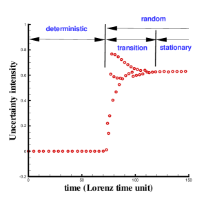
Figure 1: The uncertainty intensity $\epsilon(t)$ in case of the fluctuation of initial conditions in the normal distribution with zero mean and micro-level deviation $\sigma_{0}=10^{-30}$.

It is found that there exists such a time interval $t\in[0,T_{d}]$ with $T_{d}\approx 75$, in which $\epsilon(t)$ is so small that one can accurately predict the behavior of the dynamic system, but beyond which the uncertainty intensity increases greatly, as shown in Fig. 1. Thus, using the result at any a point $t\in(0,T_{d})$ as the initial condition and setting $t=-t$, we can gain the given observable values $x_{0},y_{0},z_{0}$ of initial conditions in a high-level of accuracy, meaning that the dynamic system looks like deterministic in $0\leq t\leq T_{d}$ and that the influence of the uncertain statistic fluctuation of initial condition is negligible. But, beyond it, the solutions become rather sensitive to the uncertain statistic fluctuation (in the level of $10^{-30}$) of initial condition and look like random, say, the micro-level uncertain statistic fluctuation in initial condition transfers into the observable macroscopic randomness. So, $T_{d}$ is an important time scale for Lorenz chaos.

As shown in Fig. 1, there exists the time $T_{s}$ with $T_{s}\approx 120$ LTU, beyond which the cumulative distribution functions (CDF) of $x(t),y(t)$, $z(t)$ and so on are approximately stationary, i.e. almost independent of the time. Besides, these CDFs are independent of the observable values $x_{0},y_{0},z_{0}$ of initial conditions, meaning that all observable information of initial conditions are lost completely. In other words, when $t>T_{d}$, the asymmetry of time seems to break down so that the time has a one-way direction, i.e. the arrow of time. It suggests that, statistically, the chaotic Lorenz system might have two completely different dynamic behaviors before and after $T_{d}$: it looks like “deterministic” without time’s arrow when $t\leq T_{d}$, but thereafter rapidly becomes random with the arrow of time. This strongly suggests that chaos might be a bridge from the micro-level uncertainty to macroscopic randomness, and thus might be an origin of macroscopic randomness and the time’s arrow. This provides us a new, different viewpoint to enrich and deepen our understandings about the SDIC of chaos.

When $T_{d}<t<T_{s}$, the CDFs of $x(t),y(t),z(t)$, their sample means and unbiased estimates of standard deviation are time-dependent, and evolve to the approximately stationary ones for $t\geq T_{s}$. This process is called the transition from the deterministic to randomness of chaos.

Write $x^{\prime}=x-<x>,y^{\prime}=y-<y>$ and $z^{\prime}=z-<z>$. It is found that the CDFs of the fluctuations $x^{\prime},y^{\prime},z^{\prime}$ are time-dependent when $t<T_{s}$ and become stationary when $t>T_{s}$. When $t>T_{d}$, the CDF of $x^{\prime}$ is different from the normal distribution with the standard deviation $<x^{\prime 2}>$, so are the CDFs of $y^{\prime}$ and $z^{\prime}$, as shown in Fig. 2. It is also found that $T_{d}$ decreases exponentially with respect to $\sigma_{0}$, the standard deviation of the tiny uncertain variables $\tilde{x}_{0},\tilde{y}_{0},\tilde{z}_{0}$ of the initial conditions. Besides, the stationary CDFs of $x^{\prime},y^{\prime},z^{\prime}$ are independent of the CDFs of $\tilde{x}_{0},\tilde{y}_{0},\tilde{z}_{0}$. In addition, more samples are needed to gain accurate mean of the high correlations of $x^{\prime},y^{\prime},z^{\prime}$, such as $<x^{\prime}z^{\prime}>,<y^{\prime}z^{\prime}>$ and especially $<x^{\prime}z^{\prime}z^{\prime}>,<x^{\prime}y^{\prime}y^{\prime}>,<y^{\prime}y^{\prime}z^{\prime}>,<y^{\prime}z^{\prime}z^{\prime}>$ and $<x^{\prime}y^{\prime}z^{\prime}>$, since the higher correlations have the larger standard derivations: this shows the difficulty to propose an accurate model for the mean $<x>,<y>,<z>$ by means of these higher correlations. This also explains why it is so difficult to propose a satisfied turbulence model valid for all kinds of turbulent flows, since Lorenz equation is a simplified model from Navier-Stokes equations. Note that, one can directly obtain all of these correlations from the Lorenz equation, as long as the number of samples are large enough. In other words, no additional models for $<x>,<y>,<z>$ are needed.

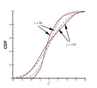
Figure 2: The CDF (solid line) of $z^{\prime}$ at $t=80$ LTU and $t=150$ LTU, compared with the corresponding normal distribution (dashed line) with the zero mean and the standard deviation $<z^{\prime 2}>$.

It is found that, given $\sigma_{0}=10^{-30}$ in case of $R=28,b=-8/3$ and $\sigma=10$, we gain exactly the same figure as shown in Fig. 1, even if we use more accurate numerical results obtained by means of the CNS with the 120-order Taylor expansion and data in the accuracy of 240-digit precision! Note that it has no physical meanings to use a micro-level deviation $\sigma_{0}$ of the initial conditions smaller than $10^{-30}$, as pointed out in the section of introduction. Thus, for chaotic dynamic systems, the transfer from micro-level uncertainty to macroscopic randomness seems unavoidable. In addition, it is fund that, in case of $b=-8/3,\sigma=10$ and $R\leq 23.54$ so that solutions are not chaotic, the micro-level uncertainty never transfers into the macroscopic level. Therefore, the SDIC of chaos is the key to such kind of transfer.

3 Conclusion and discussion

In this article, the sensitive dependence on initial condition (SDIC) of Lorenz chaos is considered together, for the first time, with the so-called continuum-assumption of fluid (on which Lorenz equations are based) from physical and statistic viewpoints. The so-called “clean numerical simulation” (CNS) proposed by Liao [6] is used to investigate the propagation of the micro-level unavoidable uncertain fluctuation (caused by the continuum-assumption of fluid) of initial conditions with chaotic solutions of Lorenz equation. Our statistic analysis based on the CNS computation of $10^{4}$ samples suggests that, due to the SDIC, the uncertainty of the micro-level statistic fluctuation of initial conditions transfers into the macroscopic randomness of chaos. This may deepen and enrich our understandings about the SDIC and chaos, from a different viewpoint of physics.

The microscopic phenomena are essentially uncertain, although probability distributions are governed by deterministic equations. However, it is traditionally believed that the micro-level uncertainty has no relationships with the macroscopic randomness. But, our statistic analysis strongly suggests that the micro-level uncertainty might be an origin of the macroscopic randomness, and chaos might be a bridge between them. Although the above conclusion is based on Lorenz equation, it has general meanings. First, we also investigated some other chaotic dynamic systems, and found the same transfer from micro-level uncertainty to macroscopic randomness for all of them. Secondly, as pointed out by Saltzman [11], the solutions of a dynamic system consist of seven nonlinear differential equations for the free convention (which is a more accurate model than Lorenz equation) are “oscillatory, overstable” (i.e. chaotic) for large enough Rayleigh number. In fact, Saltzman [11] represented the solution of the original continuous differential equations as a sum of double-Fourier components, and approximated the original problem by a set of nonlinear ordinary different equations with finite number of degree of freedom. Both of the Lorenz equation and the above mentioned system of seven equations are only special cases of it, corresponding to three and seven degree of freedom. Obviously, the larger the degree of freedom, the more accurate the model. It is found that, for large enough Rayleigh number, these dynamic systems given by Saltzman [11] with degree of freedom not less than three are chaotic, so that the micro-level uncertainty transfers into macroscopic randomness for all of them. Theoretically speaking, as the number of degree of freedom tends to infinity, this system becomes the original continuous differential equations. Thus, our conclusion about the transfer from micro-level uncertainty to macroscopic randomness has general meanings, although it is based on the Lorenz equation. This is similar to the Lorenz’s famous conclusion “long-term accurate prediction of weather is impossible” [7], which is based on the Lorenz equation, a very simple model of the N-S equation, but is correct and has been widely accepted by the scientific community.

The similar transfer has been reported in some other fields. For example, as pointed out by Bai et al [1], the disorder of materials plays a fundamental role to the so-called sample-specific behavior of fracture, i.e. the macroscopic failure may be quite different, sample to sample, under the same macroscopic condition, because the differentiation due to meso-scopic disorder may be greatly amplified and lead to largely different macroscopic effects. Xia et al [17] studied the failure of disordered materials by means of a stochastic slice sampling method with a nonlinear chain model, and found that “there is a sensitive zone in the vicinity of the boundary between the globally stable (GS) and evolution-induced catastrophic (EIC) regions in phase space, where a slight stochastic increment in damage can trigger a radical transition from GS to EIC”. In other words, the meso-scopic uncertainty of disordered materials transfers into the macroscopic randomness of failure. As mentioned by He et al [4], the nonlinearity and multi-scale might play a fundamental role in it. So, “(stochastic) fluctuations are important and must not be neglected” for the failure of disordered materials, as pointed out by Sahimi and Arbabi [10]. Another example is the evolution of the universe: the micro-level uncertainty at Big Bang, the inherent uncertainty of position and velocity of stars, and the nonlinear property of gravity might be the origin of the macroscopic randomness of the universe. All of these support our conclusion: the transfer from micro-level uncertainty to macroscopic randomness might have meanings in general.

Traditionally, it is believed that the SDIC of chaos is the origin of the so-called “butter-fly effect”: long-term prediction is impossible due to the SDIC of chaos and the impossibility of getting exact initial data with precision of arbitrary degree. This traditional idea implies that the initial data itself are exact inherently but our human-being can not obtain the exact value. However, as pointed out in this article, this traditional thought might be wrong: due to the continuum-assumption of fluid, there exists the statistic fluctuation of the initial data of Lorenz equation, no matter whether we could precisely measure the initial data or not. It should be emphasized that such kind of uncertainty is inherent: it has nothing to do with our ability. In this article, it is revealed that, due to the SDIC and the inherent uncertainty of initial data, accurate long-term prediction of chaotic solution is not only impossible in mathematics but also has no physical meanings. This provides us a new explanation of the SDIC of chaos, from the physical and statistic points of view.

The micro-level uncertainty and the physical variables $x,y,z$ of Lorenz equation are at different scales: the absolute value of the former (at the level of $10^{-30}$) is much smaller than that of the latter (at the level of 1). Unfortunately, the truncation and round-off errors (often at the level of $10^{-10}$) of most traditional numerical techniques for chaos are much larger than such kind of micro-level uncertainty, so that the propagation of the micro-level uncertainty is completely lost in the numerical noises. The CNS [6] provides us a way to accurately investigate such kind of problems with multiple scales, since the numerical noises of the CNS are much smaller than the micro-level uncertainty.

Lorenz equation is a simplified model based on the N-S equations describing flows of fluid. Note that nearly all models of turbulence are deterministic in essence: the micro-level uncertain statistic fluctuation of velocity caused by the continuum-assumption of fluid has been neglected completely. Note also that the uncertainty intensity (4) is rather similar to the definition of turbulence intensity. Since turbulence has a close relationship with chaos, it might be possible that the influence of the micro-level statistic fluctuation of velocity and temperature should be considered: we even should carefully check the theoretical foundation of turbulence and the direct numerical simulation (DNS), such as the continuum-assumption of fluid. Besides, our very fine numerical simulations and related analysis reported in this article suggest that the randomness of turbulence might come essentially from the micro-level uncertain statistic fluctuation of velocity and temperature: turbulence is such a kind of flow of fluid that it is so unstable that the micro-level uncertainty transfers into macroscopic randomness.

Hopefully, this work stimulated by a paradox could provide us some new physical insights and mathematical ways to deepen and enrich our understanding about chaos and turbulence.

References

- [1] Bai, Y. L., Ke, F.J., and Xia, M. F.: Deterministically stochastic behavior and sensitivity to initial configuration in damage fracture. Science Bulletin 39: 892 895 (1994) [in Chinese].
- [2] Egolf, D.A., Melnikov, V., Pesch, W. & Ecke, R.E.: Mechanisms of extensive spatiotemporal chaos in Rayleigh-Bènard convection. Nature, 404: 733 – 735 (2000).
- [3] Gaspard, P., Briggs, M.E., Francis, M.K., Sengers, J.V., Gammon, R.W., Dorfman, J.R. & Calabrese, R.V.: Experimental evidence for microscopic chaos. Nature, 394: 865 – 868 (1998).
- [4] He, G.W., Xia, M.F., Ke, F.J., Bai, Y.L.: Multiple-scale coupled phenomena - challenge and opportunity. Progress in Natural Science, 14: 121 – 124 (2004) [in Chinese].
- [5] Li, T.Y. & Yorke, J. A.: Period three implies Chaos. American Mathematical Monthly, 82: 985 - 992 (1975).
- [6] Liao, S.J.: On the reliability of computed chaotic solutions of non-linear differential equations. Tellus-A, 61: 550 – 564 (2009).
- [7] Lorenz, E.N.: Deterministic non-periodic flow. Journal of the Atmospheric Sciences, 20: 130 – 141 (1963).
- [8] Lorenz, E.N.: Computational periodicity as observed in a simple system. Tellus-A, 58: 549 – 559 (2006).
- [9] Poincaré, J.H.: Sur le problème des trois corps et les équations de la dynamique. Divergence des séries de M. Lindstedt. Acta Mathematica, 13:1 – 270 (1890).
- [10] Sahimi, M. and Arbabi, S.: Mechanics of disordered solid. III. Fracture properties, Physical Review B 47: 713 – 722 (1993).
- [11] Saltzman, B.: Finite amplitude free convection as an initial value problem (I). Journal of the Atmospheric Sciences, 19: 329 – 341, 1962.
- [12] Smith, P.: Explaining Chaos. Cambridge University Press, Cambridge (1998).
- [13] Tsonis, A.A.: Randomnicity: Rules and Randomness in Realm of the Infinite. Imperial College Press (2008).
- [14] Tucker, W.: The Lorenz attractor exists. C. R. Acad. Sci. 328:1197 – 1202 (1999).
- [15] Wang, P.F., Li, J.P. & Li, Q.: Computational uncertainty and the application of a high-performance multiple precision scheme to obtaining the correct reference solution of Lorenz equations. Numerical Algorithms, online (DOI: 10.1007/s11075-011-9481-6).
- [16] Werndl, C.: What are the new implications of Chaos for unpredictability? Brit. J. Phil. Sci. 60:195 – 220 (2009).
- [17] Xia, M.F., Ke, F.J., Wei, Y.J., Bai, J. and Bai, Y.L.: Evolution induced catastrophe in a nonlinear dynamical model of material failure. Nonlinear Dynamics 22: 205 – 224 (2000).