Improved Modeling of the Rossiter-McLaughlin Effect for Transiting Exoplanets
Abstract
We present an improved formula for the anomalous radial velocity of the star during planetary transits due to the Rossiter-McLaughlin (RM) effect. The improvement comes from a more realistic description of the stellar absorption line profiles, taking into account stellar rotation, macroturbulence, thermal broadening, pressure broadening, and instrumental broadening. Although the formula is derived for the case in which radial velocities are measured by cross-correlation, we show through numerical simulations that the formula accurately describes the cases where the radial velocities are measured with the iodine absorption-cell technique. The formula relies on prior knowledge of the parameters describing macroturbulence, instrumental broadening and other broadening mechanisms, but even 30% errors in those parameters do not significantly change the results in typical circumstances. We show that the new analytic formula agrees with previous ones that had been computed on a case-by-case basis via numerical simulations. Finally, as one application of the new formula, we reassess the impact of the differential rotation on the RM velocity anomaly. We show that differential rotation of a rapidly rotating star may have a significant impact on future RM observations.
1 Introduction
Transiting exoplanetary systems provide valuable opportunities to learn about the nature of the exoplanets, their orbits, and their host stars. In particular, when we measure the radial velocity (RV) of a star during a planetary transit, we see an anomalous Doppler shift (beyond the usual orbital RV) which is called the Rossiter-McLaughlin (hereafter, RM) effect (Rossiter, 1924; McLaughlin, 1924; Hosokawa, 1953; Albrecht et al., 2007). It arises because a portion of the rotating stellar disk is blocked by the planet. The partial occultation brings about a distortion in the spectral lines, which is manifested as an anomalous RV depending on the position of the planet on the stellar disk (see, e.g., Queloz et al., 2000; Ohta et al., 2005; Winn et al., 2005; Narita et al., 2007; Collier Cameron et al., 2010). The time variation of the RV anomaly reveals the (sky-projected) angle between the planetary orbital axis and the stellar spin axis. Measurements of this angle have proved to be an important observational clue to the origin of close-in giant exoplanets.
It is widely assumed that close-in gas giants, of which more than 100 are known, formed at a few AU away from their host stars and subsequently “migrated” inward (Lin et al., 1996; Lubow & Ida, 2010). Many planetary migration scenarios have been investigated, and some of them predict small values of while others allow larger spin-orbit misalignment angles (e.g., Fabrycky & Tremaine, 2007; Wu et al., 2007; Nagasawa et al., 2008; Chatterjee et al., 2008). The observed distribution of and its dependence on the host star properties (such as masses and ages) can be important clues to understand the origin of close-in giant exoplanets (Winn et al., 2010a; Fabrycky & Winn, 2009; Morton & Johnson, 2011).
Observations of the RM effect have now become almost routine (Winn, 2010; Moutou et al., 2011). However, it is important to remember that the relationship between the observed RV anomaly, and the position of the planet on the stellar disk, is not completely straightforward. This is because the RM effect is actually a spectral distortion, even though it is frequently studied as though it were a pure Doppler shift.111An alternative is to model the line profiles directly, as has been done by Albrecht et al. (2007) and Collier Cameron et al. (2010), which can be advantageous in some circumstances. Many alternatives have been pursued to calibrate the relationship between the observed signal and the underlying parameters of the planet and star. Ohta et al. (2005) and Giménez (2006) derived analytic formulas for the RV anomaly based on the computation of the first moment (the intensity-weighted mean wavelength) of distorted spectral lines. This approach is simple and convenient because the computed velocity anomaly does not depend on the intrinsic shape of spectral lines (Hirano et al., 2010), and has been useful for quick computations where high accuracy is not essential, and for gaining insight into the parameter dependence of the RM velocity anomaly. Winn et al. (2005), however, noted that the analytic formula by Ohta et al. (2005) (hereafter, the OTS formula) deviates from the results based on a more realistic numerical calibration; they simulated spectra exhibiting the RM effect for many different positions and sizes of the planet, and then analyzed the mock spectra with the same data analysis codes that are used routinely to derive precise RVs with the High Resolution Echelle Spectrometer (HIRES) installed on the Keck I telescope. As a result, they showed that the OTS formula disagrees with the numerical calibration by about 10% in terms of the RM amplitude for the case of HD 209458. For this reason, subsequent studies (e.g., Winn et al., 2005; Narita et al., 2009a) have relied upon numerical calibration of the relation between the anomalous RV and the position and size of the planet, which is done on a case-by-case basis depending on the stellar parameters.
It would be more convenient to rely on a single analytic formula than to perform these laborious numerical simulations for each system. An analytic treatment also provides insight into the reason for the limitation of the formulas of Ohta et al. (2005) and Giménez (2006). Hirano et al. (2010) took a step in this direction, pointing out that the discrepancy between the OTS formula and the simulated results was a consequence of the algorithm used to estimate the RV anomaly. While the OTS formula was derived by computing the first moment of the distorted line, in practice the RVs are computed by cross-correlating an observed spectrum with a template spectrum of the same star [e.g., for the High Accuracy Radial velocity Planet Searcher (HARPS); Triaud et al. (2009)], or by forward-modeling to fit an observed spectrum with superimposed iodine absorption lines [e.g., for the High Dispersion Spectrograph (HDS) on the Subaru telescope and Keck/HIRES; Sato et al. (2002); Butler et al. (1996)]. Using a simplified description of a single spectral line (a Gaussian function), Hirano et al. (2010) compared the RV anomalies derived by computing the first moment and by cross-correlation. They showed that the two methodologies yield different velocity anomalies, in a manner that qualitatively explains the previous numerical findings. In particular they showed that the deviations between the OTS formula and the results of cross-correlation are larger for more rapidly rotating stars.
In this work, we take the next step by developing a more realistic description of stellar line profiles, in order to derive a more accurate analytic formula. Instead of using a simple Gaussian model for a spectral line profile, we include realistic kernels for rotational broadening, macroturbulence and other effects such as instrumental broadening due to the finite resolution of a spectrograph. We test and validate the new analytic formula through various numerical simulations, and show that it is accurate enough for the real data analysis.
This paper is organized as follows. In Section 2, we derive the new analytic formula for the RM effect assuming an analytic function for the stellar line profile. We present the definitions and the result there, while the detailed derivation of the main finding is described in Appendices A and B. In order to make sure that the new analytic formula is a good approximation for the observed velocity anomaly due to the RM effect, we compare it with numerical simulations using mock transit spectra in Section 3. Also, we check on the magnitude of systematic errors due to imperfect knowledge of the parameters describing the absorption line profiles for a given star. As an application of the new analytic formula, we try to reassess the impact of stellar differential rotations on the RM velocity anomaly taking the XO-3 system as a test case in Section 4. The final section (§5) is devoted to discussion and summary.
2 Derivation of the New Analytic Formula for the RM Effect
In this section, we derive the new analytic formula that describes the velocity anomaly during a transit. We begin with our description of the stellar absorption lines. We follow the formulation by Hirano et al. (2010) but slightly change the basic equations in order to describe the stellar line profiles more realistically. Since the velocity field on the stellar surface is of primary importance, it is more convenient to express all the functions in terms of velocity rather than wavelength. In what follows, the velocity component indicates the velocity shift relative to the center of an absorption line. This is related to the wavelength shift by the usual formula , where is the central wavelength of the absorption line and is the speed of light. Following the model of spectral lines by Gray (2005), we write a stellar line shape as
| (1) |
where is the intrinsic stellar line shape in the absence of stellar rotation and macroturbulence (for which we will give an explicit expression later), and is the broadening kernel due to stellar rotation and macroturbulence222We here assume a symmetric line profile and ignore the convective blueshift (CB) effect, discussed by Shporer & Brown (2011).. The symbol indicates a convolution between two functions. Since the continuum level and the normalization factor in the spectrum do not affect the result in estimating the velocity anomaly during a transit, for convenience we subtract the continuum level so that becomes zero in the limit of . Furthermore we normalize the spectrum so that
| (2) |
The minus sign indicates that describes an absorption line. The rotational-macroturbulence broadening kernel is calculated by disk-integrating the Doppler-shift component of the stellar surface due to both stellar rotation and macroturbulence. We adopt “the radial-tangential model” for macroturbulence, for which the kernel in the absence of rotation is
| (3) |
where is the macroturbulent velocity parameter and is the angle between our line-of-sight and the normal vector to the local stellar surface (Gray, 2005, page 433). The angle is related to the coordinate (, ) on the stellar disk by
| (4) |
where the -axis is taken to be along the sky projection of the stellar spin axis, and is the radius of the star. Assuming a quadratic limb-darkening law, the disk-integrated line broadening function due to stellar rotation and macroturbulence is expressed as
| (5) |
where and are the limb-darkening coefficients, is the angular spin velocity of the star, and is the inclination angle of the stellar spin axis relative to the line of sight (Gray, 2005). The Doppler shift in the function is the consequence of stellar rotation, neglecting differential rotation. As Gray (2005) pointed out, the broadening kernel cannot be expressed as a convolution of the two different broadening kernels of the stellar rotation and the macroturbulence. As we will show, the coupling between rotational broadening and macroturbulent broadening plays an important role in estimating the velocity anomaly due to the RM effect, especially when the macroturbulent velocity is appreciable when compared to the rotational velocity of the star (see the difference between line profiles with and without macroturbulence shown in Figure 1). Indeed, this coupling between rotation and macroturbulence was neglected in the previous numerical calibrations by Winn et al. (2005) and others.
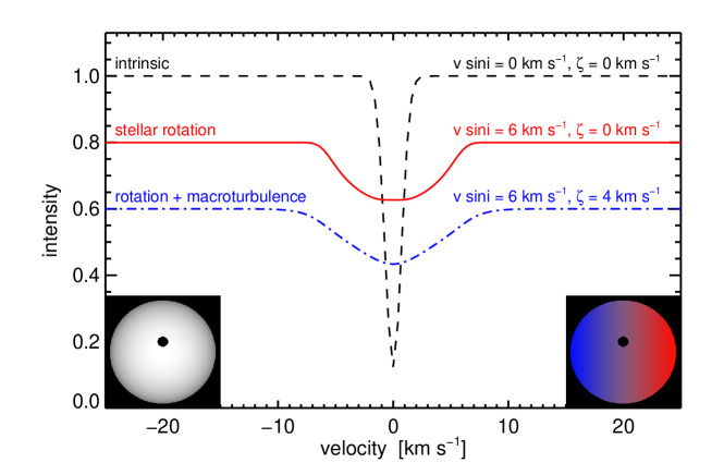
Next, we compute the line shape during a planetary transit. During a transit, the spectral contribution of the portion blocked by the planet is written as
| (6) |
where indicates a kernel similar to that given in Equation (5) but for which the disk-integration should only be performed over the blocked part of the stellar surface, rather than the entire stellar disk. As long as the planet is sufficiently small relative to the star, the Doppler shift in Equation (5) is nearly constant over the integration region. Thus, if we define as the -coordinate of the intensity-weighted center of the eclipsed portion of the star, we can remove the macroturbulence kernel from the integral and define the following two useful quantities:
| (7) | |||
| (8) |
so that becomes
| (9) |
The first quantity, , is the instantaneous fractional decrease in flux due to the transit. The second quantity, , is the rotational radial velocity of the occulted portion of the stellar disk, which is occasionally referred to as the “subplanet velocity.” With these definitions the stellar line profile during a transit is expressed as
| (10) |
It should be noted that the macroturbulent kernel remains in the modeled transit line profile. This treatment is necessary since the two effects of rotational broadening and macroturbulence are coupled with each other. In short, the line profile during a transit expressed by Equation (10) is different from the line profile modeled by Hirano et al. (2010) (Eq.[11]) in two senses: Equation (10) explicitly involves the effect of macroturbulence, and it is expressed in terms of velocity.
| Symbol | Meaning | Typical Range |
|---|---|---|
| the instantaneous fractional decrease in flux due to the transit (Eq. [7]) | 0.00 - 0.02 | |
| the subplanet velocity (Eq. [8]) | ||
| the velocity anomaly due to the RM effect | - | |
| the limb-darkening parameters for the quadratic limb-darkening law | 0.3 - 0.5 | |
| the stellar spin velocity | - | |
| the stellar effective temperature | - | |
| the inclination of the stellar spin axis measured from our line-of-sight | - | |
| the latitude on the stellar surface | ||
| the stellar radius | - | |
| the position of the transiting planet on the stellar disk | ||
| the coefficient of differendtial rotation | ||
| the Gaussian dispersion of spectral lines (Eq. [20]) | 2.5 - 4.5 km s-1 | |
| the Lorentzian dispersion of spectral lines | 0.5 - 1.5 km s-1 | |
| the macroturbulence dispersion | 2.0 - 6.5 km s-1 | |
| the angle between the line-of-sight and the normal vector to the stellar surface | - | |
| the spin-orbit misalignment angle | ||
| the microturbulence dispersion | 0.0 - 2.0 km s-1 | |
| the frequency in the Fourier domain | - | |
| the angular velocity of the stellar spin | - |
Armed with the preceding results, we now express the velocity anomaly during a transit in terms of the fractional flux decrease and the subplanet velocity . Basically, we follow Hirano et al. (2010) in order to compute the best-fit value for the anomalous RVs; they cross-correlated the spectrum during a transit with a stellar template spectrum, and then calculated the best-fit value for the velocity anomaly by maximizing the cross-correlation function :
| (11) | |||
| (12) |
To proceed further, we need a specific model for the intrinsic line shape . We here adopt the Voigt function for :
| (13) | |||||
| (14) | |||||
| (15) |
where is the thermal velocity parameter and is the Lorentzian velocity parameter (due to pressure broadening or natural broadening). These parameters are related to individual stellar properties such as the effective temperature, surface gravity, and the nature of each absorption line. Some line profiles of especially strong absorption lines (such as the Na D lines) are saturated and intrinsically different from the Voigt function in shape. However, most of the lines in the wavelength region used in RV analyses are relatively weak, by design, and are well approximated by the Voigt function in the absence of the stellar rotation and macroturbulence.
Substituting Equations (1) and (10) into Equations (11) and (12), we compute the velocity anomaly due to the RM effect. Since further calculations are mathematically complicated, we describe the detail of the derivation in Appendix A and write down the result alone:
| (16) |
where
| (17) | |||||
| (18) |
where is the Bessel function of the first kind (see also Appendix B). Equation (16) is the main finding in the present paper and will be used in the comparison with simulated results.
3 Validity of the Analytic Formula
3.1 Comparison with Numerical Simulations for Subaru/HDS
One of the major differences between the derivation of the analytic formula (Eq. [16]) and the manner in which RV data are actually analyzed is that the analytic formula is based on the cross-correlation method while the data analysis (for Subaru/HDS and Keck/HIRES at least) adopts the forward modeling method using the Iodine cell for a precise wavelength calibration. Another difference between them is that the analytic formula assumes only one absorption line in its derivation while the actual stellar spectra have many lines differing in depth, shape, and so on. Thus, in order to test the validity of Equation (16), we perform the mock data simulation described below and compare the results with the analytic formula.
3.1.1 Mock Data Simulation
The mock data simulation with the Iodine RV calibration is described in detail by Winn et al. (2005) and Narita et al. (2009a). In order to generate mock spectra during a transit, we begin with theoretically synthesized spectra by Coelho et al. (2005), whose spectral lines are modeled by incorporating thermal broadening (including microturbulence), and Lorentzian (natural or pressure) broadening. Since intrinsic line profiles depend on the stellar type, we first test the comparison for a G0 star, whose effective temperature is 6000 K. When we obtain the synthetic spectrum from the synthetic spectrum library, we assume a representative value of the surface gravity () for a G0 star with a planet and the solar abundance for metallicity ([Fe/H]=0.0).
Using the synthetic spectrum, we generate the mock spectra during a transit by the following procedure.
-
1.
We broaden the synthetic spectrum by convolving the rotational-macroturbulent kernel (Eq. [5]), so that it represents the template spectrum of the actual star. We adopt the limb-darkening parameters and (Claret, 2004), and the macroturbulence parameter km s-1 (Valenti et al., 2005). We try three different values for the rotational velocity of the star: km s-1, 5.0 km s-1, and 7.5 km s-1.
-
2.
We Doppler-shift the original unbroadened spectrum by , multiply by , and then convolve the spectrum with the macroturbulence kernel (Eq. [3]), so that the resultant spectrum represents the spectral contribution from the portion occulted by the transiting planet. For each of the three values of , we consider , 0.008, 0.012, 0.016, and 0.020. We then assign 21 different values to evenly spaced from to , yielding in total 105 different points in the grid for each value of . The macroturbulent broadening depends not only on the -coordinate but also on the -coordinate on the stellar disk (see Eqs. [3] and [4]). For simplicity, however, we assume when we generate the mock transit spectra.
-
3.
We generate the mock transit spectra by subtracting the Doppler-shifted and scaled spectra in the second step from the broadened spectra created in the first step.
-
4.
We multiply the mock transit spectra by the iodine transmission spectrum used for calibration, and convolve the Star+I2 spectrum with the representative instrumental profile of Subaru/HDS for the case of the slit width being 0.8′′, corresponding to the spectral resolution of 333The choices for the instrumental profiles used in the mock simulation are explained later..
We then take these 105 mock spectra for each of three values of , and use them as inputs to the RV analysis routine for Subaru/HDS. The RV analysis using the iodine cell is described in detail by Sato et al. (2002) (for Subaru/HDS) and Butler et al. (1996) (for Keck/HIRES). For each point of the grid, the RV analysis routine outputs a velocity anomaly due to the RM effect.
3.1.2 Results for a G0 Star
We compare the results based on the mock data simulation with the analytic expression (16). Figure 2 shows the comparison between the simulated data points and the analytic formula (Eqn. [16]). The three different panels are for the three different values of : (top) 2.5 km s-1, (middle) 5.0 km s-1, and (bottom) 7.5 km s-1. For each of the five values of , the data points indicated by color symbols show the simulated results; in black, in red, in blue, in purple, and in green.
In order to draw the analytic curves, we need to choose values of and . Although they are related to intrinsic stellar line profiles, each spectral line has its own values for and , so we need to know the “effective” values of those line parameters in order to make a comparison between the analytic formula and the simulated results. For the purpose, we employ an autocorrelation method. By autocorrelating the synthetic spectrum for a G0-type star, we obtain an effective line profile of the spectrum (see Appendix C for details). Since there is a strong degeneracy between the two stellar line parameters and , we fix based on a simple physical principle and estimate the Lorentzian dispersion from the effective line profile. In principle, the intrinsic Gaussian dispersion in each spectral line is determined by the effective temperature of the star and the “the micro-turbulence” dispersion as
| (19) |
where and are the Boltzmann constant and the mass of the atom (or molecule) in question, respectively (Gray, 2005). In addition, as we will show later, the simulated velocity anomalies also depend on the instrumental profile which we assume in generating mock spectra. Therefore, we here adopt an ad hoc assumption that the Gaussian width parameter in Equation (16) depends also on the width of the instrumental profile so that is expressed as
| (20) |
where is the dispersion of Gaussian which best-fits the representative instrumental profile adopted in observations.
Substituting eV, GeV/c2 (the mass of an iron atom444Iron lines are most numerous in the wavelength range used for the RV analysis with the iodine cell.), km s-1 (Coelho et al., 2005), and km s-1 (the dispersion of the instrumental profile of Subaru/HDS we assumed in generating mock transit spectra, corresponding to the spectral resolution of ), we obtain km s-1 and km s-1. Fitting the effective line profile with the Voigt function assuming km s-1, we obtain km s-1 (Appendix C).
In each panel (different ) of Figure 2, the analytic curves based on Equation (16) are shown in the same colors as the simulated results indicated by symbols for each value of . We adopt =(4.0 km s-1, 0.9 km s-1). The other parameters () in Equation (16) are fixed at the same values used to make mock transit spectra.
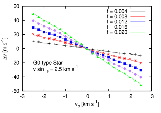
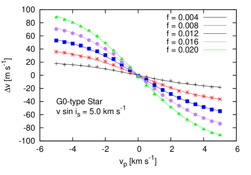
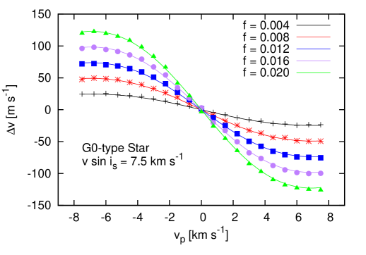
For all of the three different rotational velocities, the analytic curves are in very good agreement with the simulated results. As long as is small, the velocity anomaly curves are nearly linear and can be approximated as . As Winn et al. (2005) and other authors have pointed out, however, they are significantly curved for larger values of .
3.1.3 The Impact of Instrumental Profiles
In the forward modeling method using the iodine cell, radial velocities of a star are computed by modeling each observed spectrum with the following equation:
| (21) |
where and are the transmission spectrum of the Iodine cell and the template spectrum of the same star, respectively (Sato et al., 2002; Butler et al., 1996). Outside of a transit, the intrinsic stellar line profile of each spectrum is supposed to be the same as that of the template spectrum, and therefore is not affected by the instrumental profile which may be variable during an observation. During a transit, however, the intrinsic stellar line profile is distorted due to the partial occultation, and it is not clear if the IP affects the radial velocity including the RM velocity anomaly . Thus, in order to see if the instrumental profile used in the mock data analysis affects the RM velocity anomaly, we repeated the same mock data analysis described above, but with a different instrumental profile. In the simulation above, we have fixed the instrumental profile so that it corresponds to the spectral resolution of for Subaru/HDS. This time, we adopt the instrumental profile with the spectral resolution of . In this case, the dispersion of Gaussian fits the instrumental profile is approximately km s-1. After generating many mock spectra for , 5.0, and 7.5 km s-1 as in Section 3.1.1, we analyzed them with the usual RV routine to obtain the velocity anomaly .
In order to quantify the differences between the two cases of the instrument profile, we compute the following statistics for each case of the instrumental profiles:
| (22) |
where is the simulated velocity anomaly for each point of the grid, and is the value computed by Equation (16) as a function of , , , and . When we compute , all the parameters other than and are fixed at exactly the same values as are adopted in the numerical simulation (such as and ). The summation in the above expression is performed over the data points on the grid with three different values of . The statistics, , indicates the degree of agreement between the analytic formula and the simulated results in terms of the representative velocity anomaly . For each of the instrumental profiles ( and ), we compute , for and .
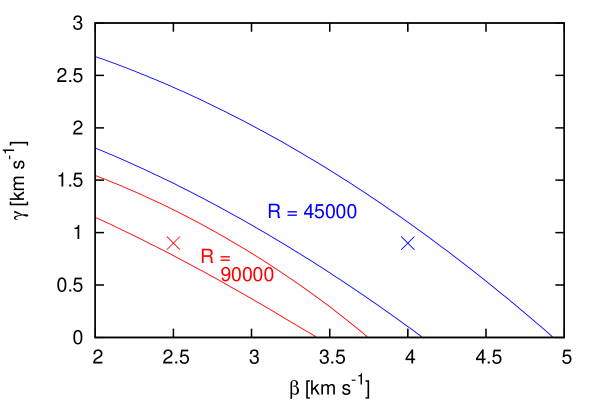
As a result of computing in the grid, we find the lowest value of is approximately 0.0045 for both of the two different instrumental profiles, representing very good agreement. For instance, the dispersion of the simulated velocity anomalies around the analytic formula is expected to be less than m s-1 in case of and km s-1. This deviation is much smaller than the usual precision with which RVs can be measured.
In Figure 3, we show contours of the goodness-of-fit statistic . The regions between the two blue curves and two red curves are where for and , respectively. Since the Gaussian and Lorentzian dispersions and strongly degenerate, the values of and that fit the simulated results well are expected to be located in extended areas. Thus, we show the “best-fit regions” where the analytic formula agrees well with the simulated results. From Figure 3, it is obvious that the best-fit region is shifted toward smaller values of when we adopt the higher spectral resolution. This result implies that the instrumental profile in spectroscopic observations does affect the velocity anomaly due to the RM effect. We interpret the results as follows; in the forward-modeling fitting procedure, the instrumental profile (a finite spectral resolution) plays a similar role as the other physical broadening mechanisms for spectral lines. For reference, we show =(4.0 km s-1, 0.9 km s-1) by the blue cross, which are the intrinsic line parameters for estimated by the spectral line analysis in Appendix C. Also, substituting km s-1 into Equation (20) for the case of , we obtain km s-1, which, along with km s-1 (the same value as used in the comparison for ), is shown in Figure 3 by the red cross. It should be emphasized that the values of shown by the blue and red crosses are estimated in a way independent of the mock data simulation (Appendix C) but are consistent with the regions where the analytic formula best agrees with the simulated results, for the two different instrumental profiles.
In summary, as a result of trying two different cases of the spectral resolution ( and 90000), we have shown that the RM velocity anomaly is actually affected by the specific choice of the instrumental profile. Since instrumental profiles are often approximated as Gaussian, we incorporate its impact on the line profile into the intrinsic Gaussian dispersion by adding the instrumental broadening in quadrature, which justifies the treatment shown in Equation (20).
3.1.4 Results for Other Spectral Types of Stars
So far, we have considered a G0 star. In order to make sure that our analytic formula is applicable for a variety of different stellar types, we consider stars with the effective temperatures of K (an F5 star) and 5000 K (a K0 star) using the theoretically synthesized spectra, just as we did for a G0 star.
- F5 star
-
In generating mock spectra for an F-type star ( K), we broaden the synthetic spectrum of an F5 star (Coelho et al., 2005) assuming the rotational velocity of , 10, and 15 km s-1. The other adopted parameters include and for the limb darkening parameters (Claret, 2004), and km s-1 for the macroturbulent velocity parameter (Gray, 2005). Except for those parameters, we perform exactly the same simulation described in Section 3.1.1. The simulated results for km s-1 are shown in the upper panel of Figure 4, along with the analytic formula (Eq. [16]) assuming km s-1, 0.9 km s-1). These Gaussian and Lorentzian dispersions are also estimated by the combination of Equation (20) adopting K, and the spectral line analysis using the auto-correlation method. Again, the analytic curves well describe the behavior of the simulated results. They are also in good agreement with each other for km s-1 and 15 km s-1, although for brevity we do not show all of those results here.
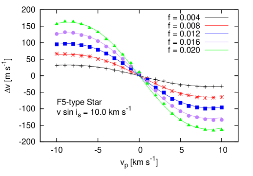
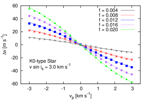
Figure 4: The comparison between simulated results (symbols) and Equation (16) (solid curves) for an F5 star with km s-1 (upper) and for a K0 star with km s-1 (lower), respectively. - K0 star
-
We also make the mock transit spectra for a K0 star ( K) and put them into the RV routine. Since most of the K-type dwarfs are relatively slow rotators, we adopt small rotational velocities: , 3.0, and 4.5 km s-1. We fix the limb-darkening parameters and the macroturbulent velocity parameter to be , (Claret, 2004), and km s-1 (Valenti et al., 2005). We compare the simulated velocity anomalies with Equation (16). As an example we show the result for km s-1 in the lower panel of Figure 4, for which we assume km s-1 and km s-1, as estimated by analyzing the synthetic line profiles for G0 and F5 stars.
All the numerical simulations show that our new analytic formula reproduces the simulated results within the current RV precisions. The agreement also suggests that we can validate the previously reported empirical relations for Subaru/HDS (i.e., Narita et al., 2009a, b, 2010a, 2010b; Hirano et al., 2011), which are based on the similar mock data simulations.
3.2 Sensitivity of the Formula to Line Parameters
In the previous subsection, we have shown that the analytic formula (Eq. [16]) gives an accurate description of the simulated velocity anomalies during a transit as long as we adopt appropriate values of and for a given type of star. However, there are several practical issues that must be addressed before the analytic formula is applied to real data analysis. First, the macroturbulent velocity parameters that we assumed in both the application of the analytic formula and in the mock data simulations will not be known a priori for real stars. Second, we have used theoretically synthesized spectra to generate mock transit spectra, but actual intrinsic line profiles in observed spectra may differ from theoretical ones. Finally, although we have adopted representative instrumental profiles in both of the analytic formula and simulation, the instrumental profile is generally dependent on many factors such as temperature variations, the position on CCD, etc, even if we adopt the same spectrograph setups for observations. Therefore, it is important to investigate the sensitivity of Equation (16) to those parameters affecting the line profile (including the instrumental profile). In this subsection, we perturb the values of those line parameters and examine the resulting changes to the outputs of the analytic formula.
3.2.1 Dependence on Macroturbulence
First we consider changes in the macroturbulence parameter. The macroturbulence dispersion for a G0-type star like HD 209458 is empirically estimated as km s-1 (Valenti et al., 2005). We here change it by with respect to that value (i.e. and 5.6 km s-1) and plot the velocity anomaly curves for HD 209458 assuming the other line parameters as km s-1,0.9 km s-1) and the stellar rotational velocity of km s-1. The top panel in Figure 5 shows the three cases of the macroturbulence dispersion: km s-1(black), 3.0 km s-1(red), and 5.6 km s-1 (blue).
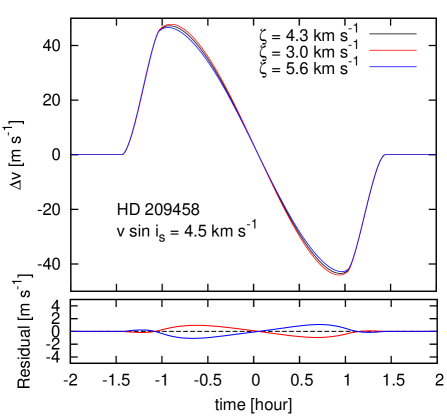
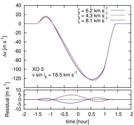
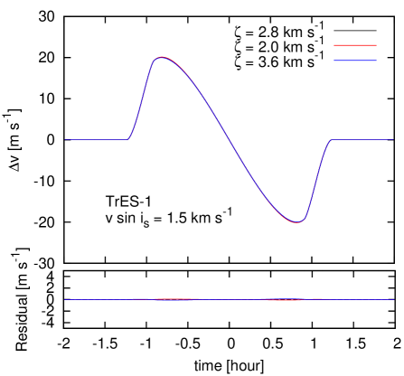
Inspection of Figure 5 shows that the RV difference between the curves is at most m s-1 ( of the representative velocity anomaly for HD 209458), which is less than the RV precision from an observational point of view. Therefore, the choice of for this type of star does not significantly affect the results.
We also show the comparisons for other two systems: XO-3 and TrES-1. For an F5 star XO-3, we adopt km s-1, km s-1, and km s-1, and try three different cases of : 4.3, 6.2, and 8.1 km s-1 (changed by around the central value). Likewise, we compute the RM velocity anomaly for TrES-1, assuming km s-1, km s-1 and km s-1. We choose values for the macroturbulence dispersion of , 2.8, and 3.6 km s-1. The results are shown in the middle and bottom panels in Figure 5. The RV differences of the colored curves from the black ones are at most 5 m s-1 ( of ) for XO-3 and 0.1 m s-1 ( of ) for TrES-1, respectively. These values are less than the RV precision that has been achieved for each system, which are approximately 8 m s-1 (Winn et al., 2009) and 10 m s-1 (Narita et al., 2007), respectively.
3.2.2 Dependence on and
Next, we focus on the Gaussian and Lorentzian components of line profiles. Fixing the values of macroturbulence parameter , we change and in Equation (16), and plot the RM curves for the three systems above. Figure 6 presents the three different cases of for HD 209458. We change both of and by from the values estimated by the spectral line analysis (Appendix C) while we fix at 4.3 km s-1. According to Figure 6, the largest discrepancy of the two colored curves from the black one is m s-1 ( of ). Although this is still comparable to or less than the RV precision for this type of stars, it is slightly larger than the difference in the curves for different (see the top panel of Figure 5).
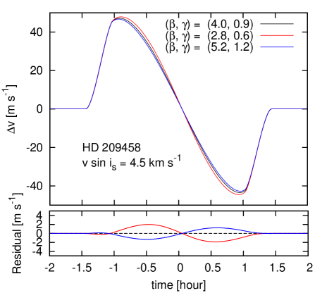
We also compare the analytic RM curves for different values of in case of XO-3 (F5-type star) and TrES-1 (K0-type star). As a result, the differences in the RM curves are at most m s-1 ( of ) for XO-3 and m s-1 for TrES-1 ( of ). These deviations are less than the current RV precision for each type of star. For a rapidly rotating star such as XO-3, the line profile is mainly determined by the stellar rotation and macroturbulence, and thus the intrinsic line profiles (thermal and Lorentzian broadening) are likely to be less important. On the other hand, for slowly rotating late-type stars as TrES-1, the intrinsic line parameters are important for describing the line shapes. However, since the RM velocity anomaly is well approximated as for narrow line profiles (slow rotators) and the velocity amplitude due to the RM effect is comparably small, an inaccurate estimation for or a variation of the instrumental profiles (less than ) are not important for slowly rotating stars.
In summary, the relative importance of the various line parameters depends on the stellar rotational velocity and the stellar type. For rapidly rotating stars ( km s-1), the macroturbulence dispersion is more important than thermal and natural profiles, while the Gaussian and Lorentzian dispersions become more significant as for moderately rotating stars (3.0 km s km s-1). Neither of the effects is important for slowly rotating stars ( km s-1).
3.3 Comparison with the Published “Calibrations” for Keck/HIRES
In Section 3.1, we compared the analytic formula with simulated results based on the analysis routine for Subaru/HDS. We have confirmed that Equation (16) well approximates the simulated results with deviations less than of the typical velocity anomaly scale (i.e. ). It is very interesting to see if the new formula (Eq. [16]) also agrees with the simulated results in previously published papers using some instrument other than Subaru/HDS. If they are shown to be consistent with each other, it suggests we no longer need to perform numerical case-by-case mock data simulations for RM analyses. If they do not agree, it may justify further investigation into which approach is more accurate. Here, we consider four systems for which the RM effect has been measured with Keck/HIRES: HAT-P-4, HAT-P-14, XO-3, and HAT-P-11. We compare Equation (16) with the published empirical relations based on mock data simulations for Keck/HIRES.
As discussed in Section 3.1.3, the instrumental profile affects the velocity anomaly due to the RM effect. Therefore, in order to make a comparison between Equation (16) and the empirical formulae, we need to know the representative dispersion of the instrumental profile of Keck/HIRES. We here adopt km s-1 in terms of velocity (a representative dispersion for the spectral resolution of ). Since other parameters are intrinsic stellar properties, we adopt similar values of , , and to the ones adopted for the comparison in Section 3.1 to draw the analytic RM curves.
| System | Empirical Relation | Reference | ||||
|---|---|---|---|---|---|---|
| HAT-P-4 | 3.2 | 0.9 | 4.1 | 5.5 | Winn et al. (2011) | |
| HAT-P-14 | 3.3 | 0.9 | 6.5 | 8.4 | Winn et al. (2011) | |
| XO-3 | 3.3 | 0.9 | 6.2 | 18.5 | Winn et al. (2009) | |
| HAT-P-11 | 3.2 | 1.1 | 2.5 | 1.5 | Winn et al. (2010b) |
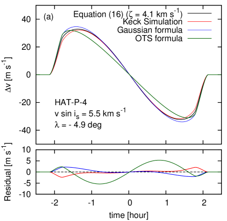
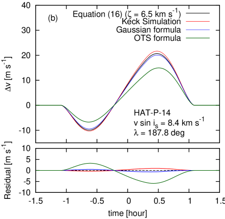
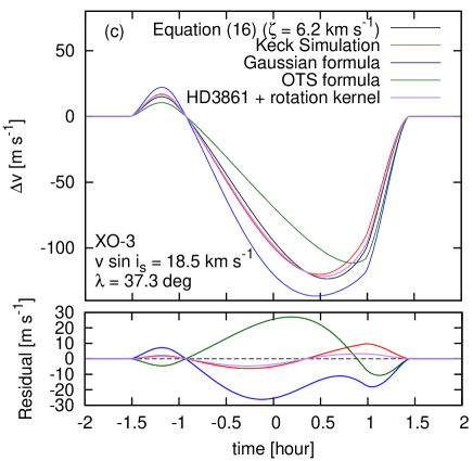
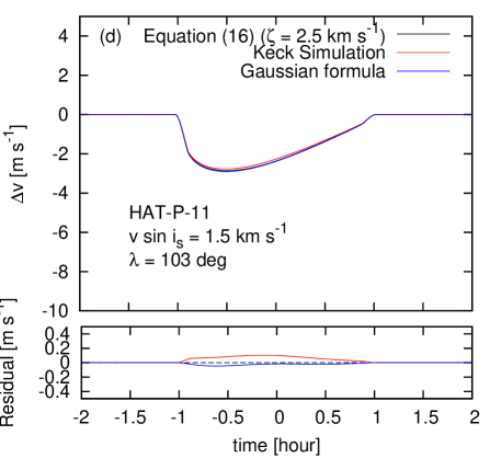
Figure 7 shows the comparison between Equation (16) and the empirical relations in literatures for the four systems. The empirical relations in the literatures are summarized in the second column of Table 2 and shown with red curves in Figure 7. Analytic curves (Eq. [16]) are shown in black. The adopted stellar line parameters to draw the analytic curves are also summarized in Table 2. In Table 2, , , , and are expressed in km s-1. For reference, we plot the Gaussian formula by Hirano et al. (2010) (i.e. Eqn.[27]) in blue and the OTS formula in green, which is expressed as . In drawing the Gaussian formula, we employ the width of the intrinsic spectral line (in the absence of stellar rotation) approximated as a single Gaussian by , where and are the values shown in Table 2.
Regarding HAT-P-4, HAT-P-14, and HAT-P-11, for which the rotational velocities are relatively small, Equation (16) and the numerical calibration formulas (red) agree within a few m s-1. For the HAT-P-11 system in particular, the two curves are almost indistinguishable. This is because Equation (16) is well approximated by for the case in which stellar lines are sufficiently narrow. On the other hand, the discrepancy between them for the case of XO-3 is more significant ( m s-1) in comparison with other systems although they are in much better agreement in comparison to the previous analytic curves based on the Gaussian and the OTS formulae.
There are at least two possible explanations for the discrepancies between Equation (16) and the Keck simulated result. First, the line parameters () adopted in Equation (16) to plot the analytic curves in Figure 7 may be significantly different from the true values for the system. Specifically, the macroturbulence dispersion is not well known for massive stars, and different values of lead to different results as we have shown in Section 3.2.1. In Section 3.1, on the other hand, we have compared Equation (16) with simulated results adopting the same values of in Equation (16) as the ones used to generate mock transit spectra.
A second possible explanation for the discrepancy between the analytic formula and the Keck simulation is that the coupling between the stellar rotation and macroturbulence (which was ignored in the numerical calibrations) has a non-negligible impact on the results. In most cases, the mock data simulations for Keck/HIRES used real observed spectra to create mock spectra during a transit. For example, to create mock spectra during a transit of the XO-3 system, Winn et al. (2009) began with the template spectrum of HD 3861, which is the same spectral type as XO-3 but has a smaller rotational velocity (F5V, km s-1). Then, they broadened that spectrum with a pure-rotational kernel to mimic the spectrum of XO-3. This is a good choice in the sense that the starting spectrum already involves the macroturbulence, which is not well known for those types of stars. However, as we have emphasized, the rotational and macroturbulence broadenings are coupled and, strictly speaking, cannot be applied sequentially. To be more precise, we should first deconvolve the spectrum with the macroturbulence before convolving with a kernel including the effects of both rotation and macroturbulence.
In order to test the second hypothesis, we perform another mock data simulation for XO-3. We begin with the F5-type synthetic spectrum and broaden it with in which we assume km s-1 and km s-1, so that the resulting spectrum mimics the template spectrum of HD 3861 (let us call it ). Then, we additionally broaden with the pure-rotational broadening kernel without macroturbulence assuming km s-1 (we call the resulting spectrum as ). This process is expected to reproduce the steps taken by Winn et al. (2009) in creating the mock spectrum of XO-3, although our starting spectrum is a theoretically synthesized one rather than that of HD 3861. By changing , we generate many mock transit spectra from and put the mock spectra into the RV analysis routine.
As a result of fitting the output velocity anomaly as a function of and , we obtain the following empirical relation:
| (23) |
where is the dispersion of the residuals of the simulated from the best-fit curve. We plot this empirical relation in Figure 7 (c) in purple. Although we still see differences between the Keck simulation (red) and our new simulation (purple), they are reduced, and the new empirical relation follows more closely the variation seen in the published numerical calibration. This suggests that part of the discrepancy (and perhaps most of the discrepancy) between Equation (16) and the Keck empirical formula is ascribed by the coupling between the stellar rotation and macroturbulence which was neglected in performing the numerical calibration. Note that the RV difference between the two simulations (red and purple) is comparable to the dispersion of our simulated results ( m s-1).
4 Impact of Differential Rotations of Stars
One of the important applications of the new analytic formula is describing the stellar differential rotation in RM measurements. Gaudi & Winn (2007) previously pointed out the impact of differential rotations via RM measurements is negligible since they are beyond the precision of the RV measurements. However, their argument on the detectability is focused on relatively slow rotators. Since the RM effect is now measured for fairly rapid rotators ( km s-1), it is important to see if the impact of stellar differential rotations is still negligible based on the precise modeling of the RM effect described in this paper. In this section, we describe the impact of stellar differential rotations in the velocity anomaly curves.
Following Reiners (2003), we model the stellar angular velocity as a function of the latitude on the stellar surface ( at the stellar equator) as
| (24) |
where is the angular velocity at the equator. The coefficient is the parameter describing the degree of differential rotation and approximately 0.2 for the case of the Sun. If the transiting planet is located at on the stellar disk, its latitude is estimated by
| (25) |
When the host star is differentially rotating, we must replace the constant in Equations (8) and (B7) with Equation (24). In this case, the degeneracy between and can be solved; for rigidly rotating systems, the velocity anomaly depends solely on , but with a differential rotation, the specific choice of the stellar inclination also affects the result.
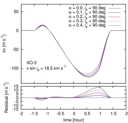
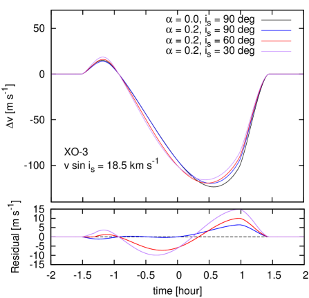
In order to evaluate the impact of differential rotations, we take XO-3 again as an example. Since the XO-3 system is reported to have a large spin-orbit misalignment and its host star has a large rotational velocity, we can expect a large impact of the differential rotation on RM velocity anomalies. Figure 8 indicates the RM anomaly curves for XO-3 with and without differential rotation. In the left panel, we change the differential rotation coefficient , fixing the stellar inclination . We try the case of , 0.1, 0.2, 0.3, and 0.4. The right panel of Figure 8 indicates the variation of the RM velocity anomaly for the different cases of , in which we set , , and while is fixed at 0.2. In this figure, the stellar spin velocity at the equator is fixed as km s-1. At the bottom of each panel, we show the residual of each curve from the black line (rigid rotation).
It is notable that the residuals are comparable to or rather larger than the RV precision for this system, which is reported to be m s-1 (Winn et al., 2009). The largest impact ( m s-1) on occurs for the case of large values of and small values of , as is expected. Figure 8 also shows that the stellar inclination significantly affects the velocity anomaly. This result, in turn, suggests that we may be able to estimate the stellar inclination from RM analyses if we can model the differential rotation for each type of stars and fix the coefficient .
5 Discussion and Summary
We have developed a new analytic formula (Eq. [16]) to describe the velocity anomaly during a planetary transit. We here summarize the previous findings describing the RM velocity anomaly along with our new analytic formula:
| (26) | |||||
| (27) | |||||
where and in Equation (27) indicate the best-fit Gaussian dispersions for the stellar template spectrum (including stellar rotation), and for the intrinsic line broadening in the absence of stellar rotation, respectively (see Hirano et al. (2010) for details). Major improvement in our new formula is that it precisely modeled various effects which can possibly affect stellar line profiles such as rotational broadening, macroturbulence, and the instrumental profile.
Numerical simulations using the mock transit spectra and the RV analysis routine for Subaru/HDS have shown that our analytic formula agrees with the simulated results within of typical RM amplitudes ( m s-1 in the case of a typical transit of a hot Jupiter).
We have also compared Equation (16) with the output of numerical calibrations of the RM effect that have been given in the literature, based on mock data simulations for Keck/HIRES. We have plotted the RM velocity anomaly curves for four existing transiting systems: HAT-P-4, HAT-P-14, XO-3, and HAT-P-11. Equation (16) proved to be in good agreement with previously reported empirical relations, although some deviations were seen for the XO-3 system. We suggest that this disagreement comes from the coupling between rotational and macroturbulent broadening, and perhaps also to imperfectly known stellar line parameters. One possible means by which this issue could be clarified is to apply our new analytic formula to observed RVs and see if Equation (16) gives a better fit to the data. We do not attempt to do so in the present paper, but we intend to reanalyze many of the existing data-sets in due course.
As Hirano et al. (2010) and others have pointed out, the relation between the position of the planet and the observed RM velocity anomaly usually does not significantly change the estimation for the spin-orbit misalignment angle since a spin-orbit misalignment is most likely to be shown by an asymmetry in the velocity anomaly curve during a transit. However, when the transit impact parameter is small, the asymmetry in the velocity anomaly curve becomes less clear and the amplitude of a series of becomes more important.
Analytic approaches to a phenomenon give us an insight into the behavior of the phenomenon, and sometimes reveals important aspects which numerical approaches are likely to overlook. We hope that our new formula will be useful in data analyses of the RM effect and make a contribution to the progress in this field.
Appendix A Derivation of the Analytic Formula (16)
In order to calculate convolutions and cross-correlations, dealing with them in the Fourier domain, where they are expressed as products, can significantly facilitate the computation. First, we Fourier-transform Equations (1) and (10) as
| (A1) | |||||
| (A2) |
where the Fourier transform of an arbitrary function is defined as
| (A3) |
so that and are explicitly given by Equations (17) and (18), respectively (see Appendix B). Thus, the Fourier transform of the cross-correlation function becomes
| (A4) | |||||
The Fourier transforms of the Gaussian and Lorentzian functions respectively are written as
| (A5) | |||||
| (A6) |
When we assume the intrinsic line profile as (the Voigt function), the Fourier transformation of becomes
| (A7) |
In this case, the inverse Fourier transformation for is expressed as
| (A8) | |||||
The derivative of Equation (A8) with respect to is
| (A9) | |||||
The maximum of the cross-correlation function is at , where
| (A10) |
Because of the exponential factors, the integrals in Equation (A) can be cut off at . Moreover, since the Gaussian width parameter is of the order of several km s-1 and the velocity anomaly is typically less than one hundred m s-1, we obtain
| (A11) |
and we can safely approximate as . Thus, using the identity for trigonometric functions:
| (A12) | |||||
we obtain following analytic formula for :
| (A13) |
Note that contrary to previously reported empirical relations, Equation (A13) implies that the velocity anomaly due to the RM effect is not proportional to the loss of flux , but the second order of slightly affects the results.
Appendix B The Fourier Transformation of the Rotational and Macroturbulence Kernel
One of the great successes in dealing with the RM effect in the Fourier domain is that the rotational and macroturbulence broadening kernel becomes significantly simpler in the Fourier domain. Here, we Fourier-transform and derive Equation (17).
Since the velocity component appears only in the macroturbulence kernel , we can write the Fourier transformation of as
| (B1) | |||||
The last expression above is expressed by a linear combination of the following form of an integral:
| (B2) |
where is a constant. The exponent in the above integrand reduces to
| (B3) |
Thus, using the Gaussian integral:
| (B4) |
Equation (B2) becomes
| (B5) |
Replacing with or , the second line in Equation (B1) is expressed as
| (B6) |
Therefore, we obtain the following expression for :
| (B7) | |||||
Since the imaginary part of the integrand in Equation (B7) is an odd function with regard to , it vanishes after integrated over . We then change variables as and , which leads to
| (B8) | |||||
where
| (B9) |
Using the following formula
| (B10) |
we obtain
| (B11) | |||||
or equivalently,
| (B12) | |||||
Appendix C Estimation of the Effective Line Profile
Here, we describe how to estimate the “effective” line profile from a spectrum. First, we model the auto-correlation function of a spectral assuming a simple analytic form of it, and then compute the actual auto-correlation function for the synthetic spectra that we use in the mock data simulation.
We assume that the synthetic spectrum (Coelho et al., 2005) is expressed by a summation of Voigt functions (defined by Eq. [13]) as
| (C1) |
where , are the equivalent width and the central wavelength of the spectral line . The Gaussian and Lorentzian dispersions of the line are also noted by and , respectively. For simplicity, we subtract the continuum (normalized to unity) of the spectrum and flip the absorption lines so that the flux takes positive values. The auto-correlation function of the spectrum is defined as
| (C2) | |||||
Since the convolution between two Voigt functions yields another Voigt function with a larger dispersion, the integral above reduces to
| (C3) | |||||
The first term in the last expression indicates the sum of all the absorption lines broadened by factors of for Gaussian and 2 for Lorentzian profiles. Here, we use this term to calculate the “effective” line profile of all the spectral lines; we define the effective Gaussian and Lorentzian dispersions and as
| (C4) |
Although a summation of Voigt functions is not necessarily expressed by a Voigt function, this treatment above is justified as long as all the values of and do not differ significantly from line to line.
The second and third terms in Equation (C3) mean the correlations between the lines separated by . It is plausible to assume that this separation is distributed randomly in a spectrum. In this case, the second and third terms become the summations of a bunch of Voigt functions centered at randomly placed . Assuming the number of spectral lines is large enough (), the second and third terms altogether becomes almost constant as a function of 555In reality, since we deal with a limited wavelength range of the spectrum, the auto-correlation function slowly decreases as a function of .. Therefore, we can approximate Equation (C3) around as
| (C5) |
where is the constant originated from the second and third terms in Equation (C3).
Next, we try to compute the auto-correlation function for the actual synthetic spectra we use to generate the mock transit spectra. We take the G0-type spectrum described in Section 3.1.1, subtract the continuum, and flip the lines. Then, we compute the auto-correlation function defined as Equation (C2). Note that we cut the spectrum so that it ranges from to , where precise radial velocity analyses are usually performed.
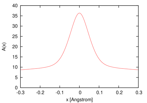
Figure 9 shows the resultant auto-correlation function of the synthetic spectrum for a G0-type star used in the mock data simulation around . As is expected from the above theoretical prediction, it has a strong Voigt-shaped peak at with an offset due to the correlations with neighboring lines. We fit this auto-correlation function assuming a form of Equation (C5). Since the Gaussian and Lorentzian dispersion and are strongly correlated, we fix as km s-1, which is calculated by Equation (19), and let only , , and be free. As a result, we find the best-fit value of as km s-1. In this paper, we use these values in comparing the analytic formula with the simulated results for a G0-type star.
References
- Albrecht et al. (2007) Albrecht, S., Reffert, S., Snellen, I., Quirrenbach, A., & Mitchell, D. S. 2007, A&A, 474, 565
- Butler et al. (1996) Butler, R. P., Marcy, G. W., Williams, E., McCarthy, C., Dosanjh, P., & Vogt, S. S. 1996, PASP, 108, 500
- Chatterjee et al. (2008) Chatterjee, A., Sarkar, A., Barat, P., Mukherjee, P., & Gayathri, N. 2008, ApJ, 686, 580
- Claret (2004) Claret A. 2004, A&A, 428, 1001
- Coelho et al. (2005) Coelho, P., Barbuy, B., Melndez, J., Schiavon, R. P., & Castilho, B. V. 2005, A&A, 443, 735
- Collier Cameron et al. (2010) Collier Cameron, A., Guenther, E., Smalley, B., McDonald, I., Hebb, L., Andersen, J., Augusteijn, Th., Barros, S. C. C., Brown, D. J. A., Cochran, W. D., Endl, M., Fossey, S. J., Hartmann, M., Maxted, P. F. L., Pollacco, D., Skillen, I., Telting, J., Waldmann, I. P., & West, R. G. 2010, MNRAS, 407, 507
- Fabrycky & Tremaine (2007) Fabrycky, D., & Tremaine, S. 2007, ApJ, 669, 1298
- Fabrycky & Winn (2009) Fabrycky, D. C., & Winn, J. N. 2009, ApJ, 696, 1230
- Gaudi & Winn (2007) Gaudi, B. S., & Winn, J. N. 2007, ApJ, 655, 550
- Giménez (2006) Giménez, A. 2006, ApJ, 650, 408
- Gray (2005) Gray, D. F. 2005, The Observation and Analysis of Stellar Photospheres (3rd ed.; Cambridge University Press.)
- Hirano et al. (2010) Hirano, T., Suto, Y., Taruya, A., Narita, N., Sato, B., Johnson, J. A., & Winn, J. N. 2010, ApJ, 709, 458
- Hirano et al. (2011) Hirano, T., Narita, N., Shporer, A., Sato, B., Aoki, W., & Tamura, M. 2011, PASJ, 63, S531
- Hosokawa (1953) Hosokawa, Y. 1953, PASJ, 5, 88
- Lin et al. (1996) Lin, D. N. C., Bodenheimer, P., & Richardson, D. C. 1996, Nature, 380, 606
- Lubow & Ida (2010) Lubow, S. H., & Ida, S. 2010, arXiv:1004.4137
- McLaughlin (1924) McLaughlin, D. B. 1924, ApJ, 60, 22
- Morton & Johnson (2011) Morton, T. D., & Johnson, J. A. 2011, ApJ, 729, 138
- Moutou et al. (2011) Moutou, C., Diaz, R. F., Udry, S., Hebrard, G., Bouchy, F., Santerne, A., Ehrenreich, D., Arnold, L., Boisse, I., Bonfils, X., Delfosse, X., Eggenberger, A., Forveille, T., Lagrange, A., Lovis, C., Martinez, P., Pepe, F., Perrier, C., Queloz, D., Santos, N. C., Segransan, D., Toublanc, D., Troncin, J., Vanhuysse, M., & Vidal-Madjar, A. 2011, A&A, in press
- Nagasawa et al. (2008) Nagasawa, M., Ida, S., & Bessho, T. 2008, ApJ, 678, 498
- Narita et al. (2007) Narita, N., Enya, K., Sato, B., Ohta, Y., Winn, J. N., Suto, Y., Taruya, A., Turner, E. L., Aoki, W., Yoshii, M., Yamada, T., & Tamura, Y. 2007, PASJ, 59, 763
- Narita et al. (2009a) Narita, N., Hirano T., Sato B., Winn, J. N., Suto, Y., Turner, E. L., Aoki, W., Tamura, M., & Yamada, T. 2009a, PASJ, 61, 991
- Narita et al. (2009b) Narita, N., Sato, B., Hirano, T., & Tamura, M. 2009b, PASJ, 61, L35
- Narita et al. (2010a) Narita, N., Sato, B., Hirano, T., Winn, J. N., Aoki, W., & Tamura, M. 2010, PASJ, 62, 653
- Narita et al. (2010b) Narita, N., Hirano, T., Sanchis-Ojeda, R., Winn, J. N., Holman, M. J., Sato, B., Aoki, W., & Tamura, M. 2010b, PASJ, 62, L61
- Ohta et al. (2005) Ohta, Y., Taruya, A., & Suto Y. 2005, ApJ, 622, 1118
- Queloz et al. (2000) Queloz, D., Eggenberger, A., Mayor, M., Perrier, C., Beuzit, J. L., Naef, D., Sivan, J. P., & Udry, S. 2000, A&A, 359, L13
- Reiners (2003) Reiners, A. 2003, A&A, 408, 707
- Rossiter (1924) Rossiter, R. A. 1924, ApJ, 60, 15
- Sato et al. (2002) Sato, B., Kambe, E., Takeda, Y., Izumiura, H., & Ando, H. 2002, PASJ, 54, 873
- Shporer & Brown (2011) Shporer, A., & Brown, T. 2011, 733, 30
- Valenti et al. (2005) Valenti, J. A., & Fischer, D. A. 2005, ApJ Supplement Series, 159, 141
- Triaud et al. (2009) Triaud, A. H. M. J., et al. 2009, A&A, 506, 377
- Winn et al. (2005) Winn, J. N., Noyes, R. W., Holman, M. J., Charbonneau, D., Ohta, Y., Taruya, A., Suto, Y., Narita, N., Turner, E. L., Johnson, J. A., Marcy, G. W., Butler, R. P., & Vogt S. S. 2005, ApJ, 631, 1215
- Winn et al. (2009) Winn, J. N., Johnson, J. A., Fabrycky, D., Howard, A. W., Marcy, G. W., Narita, N., Crossfield, I. J., Suto, Y., Turner, E. L., Esquerdo, G., & Holman, M. J. 2009, ApJ, 700, 302
- Winn (2010) Winn, J. N. 2010, arXiv:1001.2010
- Winn et al. (2010a) Winn, J. N., Fabrycky, D., Albrecht, S., & Johnson, J. A. 2010a, ApJL, 718, L145
- Winn et al. (2010b) Winn, J. N., Johnson, J. A., Howard, A. W., Marcy, G. W., Isaacson, H., Shporer, A., Bakos, G. Á., Hartman, J. D., & Albrecht, S. 2010b, ApJL, 723, L223
- Winn et al. (2011) Winn, J. N., Howard, A. W., Johnson, J. A., Marcy, G. W., Isaacson, H., Shporer, A., Bakos, G. Á., Hartman, J. D., Holman, M. J., Albrecht, S., Crepp, J. R., & Morton, T. D. 2011, ApJ, 141, 63
- Wu et al. (2007) Wu, Y., Murray, N. W., & Ramsahai, J. M. 2007, ApJ, 670, 820