SDSS DR7 superclusters

Abstract

Context. The study of superclusters of galaxies helps us to understand the formation, evolution, and present-day properties of the large-scale structure of the Universe.

Aims. We use data about superclusters drawn from the SDSS DR7 to analyse possible selection effects in the supercluster catalogue, to study the physical and morphological properties of superclusters, to find their possible subsets, and to determine scaling relations for our superclusters.

Methods. We apply principal component analysis and Spearman’s correlation test to study the properties of superclusters.

Results. We have found that the parameters of superclusters do not correlate with their distance. The correlations between the physical and morphological properties of superclusters are strong. Superclusters can be divided into two populations according to their total luminosity: high-luminosity ones with $L_{g}>400$ $10^{10}h^{-2}L_{\sun}$, and low-luminosity systems. High-luminosity superclusters form two sets, which are more elongated systems with the shape parameter $K_{1}/K_{2}<0.5$ and less elongated ones with $K_{1}/K_{2}>0.5$. The first two principal components account for more than 90% of the variance in the supercluster parameters. We use principal component analysis to derive scaling relations for superclusters, in which we combine the physical and morphological parameters of superclusters.

Conclusions. The first two principal components define the fundamental plane, which characterises the physical and morphological properties of superclusters. Structure formation simulations for different cosmologies, and more data about the local and high redshift superclusters are needed to understand the evolution and the properties of superclusters better.

1 Introduction

The large-scale distribution of the dark and baryonic matter in the Universe can be described as the cosmic web – the network of galaxies, groups, and clusters of galaxies connected by filaments (Joeveer et al. 1978; Gregory & Thompson 1978; Zeldovich et al. 1982; de Lapparent et al. 1986). In this network superclusters are the largest density enhancements formed by the density perturbations on a scale of about 100 $h^{-1}$ Mpc ($H_{0}=100h\mathrm{km\,s^{-1}Mpc^{-1}})$. Numerical simulations show that high-density peaks in the density distribution (the seeds of supercluster cores) are seen already at very early stages of the formation and evolution of structure (Einasto 2010). These are the locations of the formation of the first objects in the Universe (e.g. Venemans et al. 2004; Mobasher et al. 2005; Ouchi et al. 2005; Hatch et al. 2011). Studying the properties of superclusters helps us to understand the formation, evolution, and properties of the large-scale structure of the Universe (Hoffman et al. 2007; Araya-Melo et al. 2009a; Bond et al. 2010, and references therein). Comparison of observed and simulated superclusters, especially extreme systems among them, is a test of cosmological models (Kolokotronis et al. 2002; Einasto et al. 2007a, e; Araya-Melo et al. 2009a; Einasto et al. 2011b; Sheth & Diaferio 2011).

The first step in supercluster studies is to compile supercluster catalogues, which serve as observational databases. Supercluster catalogues have been constructed using the friend-of-friend method or using a smoothed density field of galaxies. The first method has been applied to the data on rich (Abell) clusters of galaxies to obtain catalogues of superclusters of rich clusters, both from observations and simulations (Zucca et al. 1993; Einasto et al. 1994; Kalinkov & Kuneva 1995; Einasto et al. 1997, 2001; Wray et al. 2006). Density field superclusters have been determined using data of deep surveys of galaxies (Basilakos 2003; Einasto et al. 2003a; Erdoğdu et al. 2004; Einasto et al. 2006, 2007b; Liivamägi et al. 2010; Costa-Duarte et al. 2011; Luparello et al. 2011). The properties of superclusters have been studied, for example, by Jaaniste et al. (1998), Kolokotronis et al. (2002), Costa-Duarte et al. (2011), Luparello et al. (2011), Wray et al. (2006), and Einasto et al. (2001, 2007a, 2007c, 2007e, 2011a). These studies show that the properties of superclusters are correlated. More luminous superclusters are richer and larger, contain richer galaxy clusters, and have higher maximum densities of galaxies than less luminous systems. High-luminosity superclusters are more elongated and have more complicated inner structure than low-luminosity ones.

In the present paper we use the Spearman’s correlation test and the principal component analysis (PCA), an excellent tool for multivariate data analysis, to investigate how strong the correlations between the properties of superclusters are. Our goals are to analyse the presence of possible distance-dependent selection effects in the supercluster catalogue, to study the correlations between the physical and morphological properties of superclusters, to find the possible subsets and outliers of superclusters, and to determine the scaling relations for the superclusters.

Principal component analysis have been used in astronomy for a number of purposes: the study of the properties of stars (Tiit & Einasto 1964; Deeming 1964), spectral classification of galaxies (Sánchez Almeida et al. 2010, and references therein), morphological classification of galaxies (Coppa et al. 2010), studies of galaxies, galaxy groups, and dark matter haloes (Efstathiou & Fall 1984; Lanzoni et al. 2004; Ferreras et al. 2006; Woo et al. 2008; Chang et al. 2010; Ishida & de Souza 2011; Toribio et al. 2011; Skibba & Maccio’ 2011; Jeeson-Daniel et al. 2011, and references therein), for the Hubble parameter reconstruction (Ishida & de Souza 2011, and references therein), and for studies of star formation history in the universe using gamma ray bursts (Ishida et al. 2011). Our study is the first in which the PCA is applied to explore the properties of superclusters of galaxies.

In Sect. 2 we give data about superclusters. In Sect. 3 we describe the PCA and the Spearman’s correlation test, and apply them in Sect. 4 to study the physical and morphological properties of superclusters and to derive scaling relations for the superclusters. We discuss selection effects in Sect. 5 and give our conclusions in Sect. 6.

We assume the standard cosmological parameters: the Hubble parameter $H_{0}=100\leavevmode\nobreak\ h$ km s^-1 Mpc^-1, the matter density $\Omega_{\rm m}=0.27$, and the dark energy density $\Omega_{\Lambda}=0.73$.

2 Data

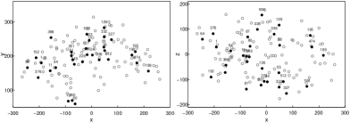
Figure 1: The distribution of superclusters in cartesian coordinates, in units of $h^{-1}$ Mpc. The filled circles denote superclusters with the luminosity $L_{g}>400$ $10^{10}h^{-2}L_{\sun}$, empty circles denote less luminous superclusters. The numbers are ID’s of luminous supercluster from L10 (Table LABEL:tab:basicscl).

We selected the MAIN galaxy sample of the 7th data release of the Sloan Digital Sky Survey (Adelman-McCarthy et al. 2008; Abazajian et al. 2009) with the apparent $r$ magnitudes $12.5\leq r\leq 17.77$, excluding duplicate entries. The sample is described in detail in Tago et al. (2010), hereafter T10. We corrected the redshifts of galaxies for the motion relative to the CMB and computed the co-moving distances (Martínez & Saar 2002) of galaxies.

We calculated the galaxy luminosity density field to reconstruct the underlying mass distribution. To determine superclusters (extended systems of galaxies) in the luminosity density field we created a set of density contours by choosing a density threshold and define connected volumes above a certain density threshold as superclusters. In order to choose proper density levels to determine individual superclusters, we analysed the density field superclusters at a series of density levels. As a result we used the density level $D=5.0$ (in units of mean density; mean luminosity density of our sample is $\ell_{\mathrm{mean}}$ = 1.526$\cdot 10^{-2}$ $\frac{10^{10}h^{-2}L_{\odot}}{(h^{-1}\mathrm{Mpc})^{3}})$ to determine individual superclusters. At this density level superclusters in the richest chains of superclusters in the volume under study still form separate systems; at lower density levels they join into huge percolating systems. At higher threshold density levels superclusters are smaller and their number decreases.

In our flux-limited catalogue the luminosity-dependent selection effects are the smallest at the distance interval 90 $h^{-1}$ Mpc $\leq D_{\mathrm{com}}\leq$ 320 $h^{-1}$ Mpc. For the present study we chose superclusters of galaxies in this distance interval. There are 125 superclusters in the sample. Even the poorest systems in our sample contain several groups of galaxies. These systems can be compared with the Local supercluster containing one cluster of galaxies with outgoing filaments. In the Appendix A we give the details of the calculations of galaxy luminosities and of the luminosity density field, as well as of the selection effects. The description of the supercluster catalogues is given in Liivamägi et al. (2010, hereafter L10).

The superclusters can be characterised by the following physical parameters: the total weighted luminosity of galaxies in a supercluster, $L_{g}$, the volume $Volume$, the diameter $Diameter$, and the number of galaxies in superclusters, $N_{\mbox{gal}}$. The supercluster volume is calculated from the density field as the number of connected grid cells multiplied by the cell volume:

$$Volume=N_{scl}\Delta^{3},$$ (1)

where $\Delta$ is the grid cell length.

The total luminosity of the superclusters $L_{g}$ is calculated as the sum of weighted galaxy luminosities:

$$L_{g}=\sum_{\mathrm{gal}\in\mathrm{scl}}W_{L}(d_{\mathrm{gal}})L_{\mathrm{gal}}.$$ (2)

Here the $W_{L}(d_{\mathrm{gal}})$ is the distance-dependent weight of a galaxy (the ratio of the expected total luminosity to the luminosity within the visibility window). We describe the calculation of weights in Appendix A. The diameter of a supercluster is defined as the maximum distance between its galaxies. The distance of a supercluster is the distance to it’s density maximum. The peak density $D_{\mbox{peak}}$ is that of the highest density peak within the supercluster. Usually the highest values of densities coincide with the richest cluster of galaxies in a supercluster. For details we refer to L10.

The overall morphology of a supercluster is described by the shapefinders $K_{1}$ (planarity) and $K_{2}$ (filamentarity), and their ratio, $K_{1}$/$K_{2}$ (the shape parameter). The shapefinders are calculated using the volume, area, and integrated mean curvature of a supercluster; they contain information both about the sizes of superclusters and about their outer shape. Systems with different shapes and similar sizes have different shape parameters (Einasto et al. 2008). For the first time the shapefinders were applied in the studies of galaxy systems by Basilakos et al. (2001) who analysed the shapes of the PSCz superclusters. We use the maximum value of the fourth Minkowski functional $V_{3}$ (the clumpiness) to characterise the inner structure of the superclusters. The larger the value of $V_{3}$, the more complicated the inner morphology of a supercluster is; superclusters may be clumpy, and they also may have holes or tunnels in them (Einasto et al. 2007e, 2011b).The formulae for the Minkowski functionals and shapefinders are given in App.B.

The large-scale distribution of superclusters is shown in Fig. 1 in cartesian coordinates. These coordinates are defined as in Park et al. (2007) and in Liivamägi et al. (2010):

$$\begin{array}[]{l}x=-d\sin\lambda,\\[3.0pt] y=d\cos\lambda\cos\eta,\\[3.0pt] z=d\cos\lambda\sin\eta,\end{array}$$

where $d$ is the comoving distance, and $\lambda$ and $\eta$ are the SDSS survey coordinates. Einasto et al. (2011a) gave detailed description of the large-scale distribution of rich superclusters.

3 Principal component analysis

Figure 2: Distribution of the standardised physical parameters of superclusters. From left to right: the total weighted luminosity of galaxies $L_{g}$, the volume and the diameter of superclusters, the density of the highest density peak inside superclusters, $D_{\mbox{peak}}$, and the number of galaxies in superclusters, $N_{\mbox{gal}}$.

The idea of the principal component analysis is to find a small number of linear combinations of correlated parameters to describe most of the variation in the dataset with a small number of new uncorrelated parameters. The PCA transforms the data to a new coordinate system, where the greatest variance by any projection of the data lies along the first coordinate (the first principal component), the second greatest variance – along the second coordinate, and so on. There are as many principal components as there are parameters, but typically only the first few are needed to explain most of the total variation.

Principal components PC$x$ ($x\in\mathbb{N}$, $x\leq N_{tot})$ are a linear combination of the original parameters:

$$PCx=\sum_{i=1}^{N_{\mathrm{tot}}}a(i)_{x}V_{i}$$ (3)

where $-1\leq a(i)_{x}\leq 1$ are the coefficients of the linear transformation, $V_{i}$ are the original parameters and $N_{\mathrm{tot}}$ is the number of the original parameters.

PCA is suitable tool to study simultaneously correlations between a large number of parameters, for finding subsets in data, and detecting outliers. Linear combinations of principal components can be used to reproduce parameters characterising objects in the dataset.

Principal components can be used to derive scaling relations. If data points lie along a plane, defined by the first two principal components, then the scaling relations along this plane are defined by the third principal component (Efstathiou & Fall 1984). For the analysis we use standardised parameters, centred on their means ($V_{i}-\overline{V_{i}})$ and normalised (divided by their standard deviations, $\sigma(V_{i}))$. Therefore we obtain for the scaling relations:

$$\sum_{i=1}^{N_{\mathrm{tot}}}a(i)_{3}\frac{(V_{i}-\overline{V_{i}})}{\sigma(V_{i})}=0.$$ (4)

For PCA, the parameters should be normally distributed. Therefore we use the logarithms of parameters in most cases; this makes the distributions more gaussian, and the range over which their values span are smaller, especially for luminosities and volumes. We do not use logarithms of morphological data, in order to not to exclude from the analysis those with negative values of shapefinders, which may occur in the case of compact superclusters with a complex overall morphology (Einasto et al. 2008, 2011b). Figures 2 and 3 show the distribution of the values of the standardised parameters. Deviations from the normal distribution are mostly caused by the most luminous (or by the poorest for the shape parameter) superclusters in our sample. In Table LABEL:tab:msd we give the mean values and standard deviations of supercluster parameters. For poor superclusters of “spider” morphology the shape parameter is not always well defined (Einasto et al. 2011a). For five systems the value of the shape parameter $|K_{1}/K_{2}|>4$; therefore we also calculated the mean value and standard deviation of the shape parameter without these systems (denoted as $K_{1}/K_{2}^{*}$). This effect does not affect the values of other parameters, thus we did not exclude these systems from our calculations.

We present in tables the values of principal components and the standard deviations, proportion of variance, and cumulative variance of principal components. The values of components show the importance of the original parameters in each PCx. We plot the principal planes for superclusters. For the calculations we used command prcomp from R, an open-source free statistical environment developed under the GNU GPL (Ihaka & Gentleman 1996, http://www.r-project.org).

To study correlations between properties of superclusters, we applied Spearman’s rank correlation test, in which the value of the correlation coefficient $r$ shows the presence of correlation ($r=1$ for perfect correlation), anticorrelation ($r=-1$ for perfect anticorrelation), or the absence of correlations when $r\approx 0$.

Table 1: Mean values and standard deviations of supercluster parameters.

(1)	(2)	(3)
Parameter	$mean$	$sd$
$\log(L_{g})$	2.367	0.378
$\log(Volume)$	2.813	0.571
$\log(Diameter)$	1.179	0.258
$\log(D_{\mbox{peak}})$	0.856	0.119
$\log(N_{\mbox{gal}})$	2.219	0.435
$\log(Dist.)$	2.379	0.113
$V_{3}$	1.770	1.185
$K_{1}$	0.015	0.031
$K_{2}$	0.027	0.069
$K_{1}/K_{2}$	-0.050	3.701
$K_{1}/K_{2}^{*}$	0.338	0.756

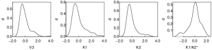
Figure 3: Distribution of the standardised morphological parameters of superclusters. From left to right: the maximum value of the fourth Minkowski functional $V_{3}$, the planarity $K_{1}$, the filamentarity $K_{2}$, and the shape parameter of superclusters, $K_{1}/K_{2}^{*}$.

4 Results

4.1 PCA with physical parameters of superclusters

We start the calculations of principal components using physical characteristics of superclusters and their distances. Including the supercluster distances may show possible correlations between the other parameters of superclusters and their distance, which will indicate that the parameters of superclusters are affected by distance-dependent selection effects.

Table 2: Results of the principal component analysis, with the distances of superclusters included.

(1)	(2)	(3)	(4)
	PC1	PC2	PC3
$\log(N_{\mbox{gal}})$	-0.444	0.264	-0.108
$\log(L_{g})$	-0.455	-0.149	-0.097
$\log(Diameter)$	-0.441	-0.133	-0.542
$\log(Volume)$	-0.454	-0.126	-0.042
$\log(D_{\mbox{peak}})$	-0.427	-0.062	0.825
$\log(Distance)$	0.100	-0.932	0.012
Importance of components
	PC1	PC2	PC3
Standard deviation	2.148	1.046	0.466
Proportion of Variance	0.769	0.182	0.036
Cumulative Proportion	0.769	0.951	0.987

Table 3: Results of the Spearman’s rank correlation test.

(1)	(2)	(3)
Parameters	$r$	$p$
$\log(Dist.)$ vs. $\log(L_{g})$	-0.06	0.50
$\log(Dist.)$ vs. $\log(N_{\mbox{gal}})$	-0.49	$9.8e-9$
$\log(Dist.)$ vs. $\log(Diameter)$	-0.11	0.20
$\log(Dist.)$ vs. $\log(Volume)$	-0.08	0.40
$\log(Dist.)$ vs. $\log(D_{\mbox{peak}})$	-0.09	0.33
$\log(Dist.)$ vs. $V_{3}$	-0.03	0.78
$\log(Dist.)$ vs. $K_{1}$	-0.08	0.37
$\log(Dist.)$ vs. $K_{2}$	0.04	0.70
$\log(Dist.)$ vs. $K_{1}/K_{2}$	-0.05	0.58
$\log(L_{g})$ vs. $\log(N_{\mbox{gal}})$	0.88	$<2.2e-16$
$\log(L_{g})$ vs. $\log(Diameter)$	0.95	$<2.2e-16$
$\log(L_{g})$ vs. $\log(Volume)$	0.98	$<2.2e-16$
$\log(L_{g})$ vs. $\log(D_{\mbox{peak}})$	0.94	$<2.2e-16$
$\log(L_{g})$ vs. $V_{3}$	0.75	$<2.2e-16$
$\log(L_{g})$ vs. $K_{1}$	0.89	$<2.2e-16$
$\log(L_{g})$ vs. $K_{2}$	0.82	$<2.2e-16$
$\log(L_{g})$ vs. $K_{1}/K_{2}$	0.19	0.04

Table LABEL:tab:pca90dist presents the results of this analysis. We show the values of only the first three principal components, enough for this test. The coefficients of the first principal component of the physical parameters are of almost equal value, while the coefficient corresponding to the distance is very small – the first principal component accounts for most of the variance of the physical parameters of superclusters. The second principal component accounts for most of the variance of the distances of superclusters. This shows that the physical parameters of superclusters are not correlated with distance. To ensure that this interpretation is correct we carried out the Spearman’s tests for correlations (Table LABEL:tab:rank). These tests showed a weak anticorrelation between the distance and the number of galaxies in superclusters, with a high statistical significance. This is not surprising since the catalogue of superclusters is based on the flux-limited sample in which the number of galaxies in superclusters depends on the distance. The sample of superclusters was chosen from a relatively narrow distance interval, so this dependence is weak. For other parameters of superclusters (luminosity, diameter, volume, and peak density), the tests showed a very weak correlation with distance (Spearman’s rank $r\approx 0.1$ or less), but with no statistical significance, as the $p$-values show. Therefore we conclude that there are no correlations between the distances and physical parameters of superclusters, and the distance-dependent selection effects have been properly taken into account when generating the supercluster catalogue and calculating the physical properties of superclusters.

Table 4: Results of the principal component analysis for the physical parameters.

(1)	(2)	(3)	(4)	(5)	(6)
	PC1	PC2	PC3	PC4	PC5
$\log(N_{\mbox{gal}})$	-0.439	0.056	0.895	-0.036	-0.018
$\log(L_{g})$	-0.460	0.112	-0.217	-0.047	0.851
$\log(Diameter)$	-0.445	0.557	-0.238	0.561	-0.344
$\log(Volume)$	-0.458	0.058	-0.268	-0.761	-0.367
$\log(D_{\mbox{peak}})$	-0.430	-0.818	-0.149	0.319	-0.144
Importance of components
	PC1	PC2	PC3	PC4	PC5
St. deviation	2.139	0.467	0.377	0.193	0.161
Prop. Variance	0.915	0.043	0.028	0.007	0.005
Cum. Proportion	0.915	0.958	0.987	0.994	1.000

We will proceed with the analysis of superclusters, taking only the physical parameters into account. Table LABEL:tab:pca90, which presents the results of this analysis, demonstrates that the coefficients of the first principal component are almost equal for different parameters of superclusters. Therefore the parameters, which describe the full supercluster (the luminosity, richness, diameter, and volume), are almost equally important in determining the supercluster properties. The cumulative variance in Table LABEL:tab:pca90 shows that the first two principal components account for more than 95% of the total variance in this supercluster sample. The first principal component accounts for most of the variance of the overall parameters of superclusters. The values of the second principal component show that the largest remaining variance in the sample comes from the peak density of superclusters. The values of the third principal component show that the coefficients corresponding to the luminosity, volume, and diameter have almost equal negative values, while the number of galaxies has large positive coefficients.

The PCA therefore suggests that the physical parameters of superclusters are strongly correlated. We checked for the presence of the correlations between the parameters with Spearman’s tests, which showed that the correlations between the parameters of superclusters are statistically of very high significance, both between the overall parameters of superclusters and between the overall parameters and the peak density inside the superclusters (Table LABEL:tab:rank). We only present the correlations between the luminosity and other parameters, to keep Table LABEL:tab:rank short. The results of the tests of other correlations are similar. Especially tight are the correlations between the luminosities, the diameters, and the volumes of superclusters, as the correlation coefficients show in Table LABEL:tab:rank.

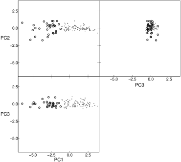
Figure 4: Principal planes for superclusters, PCA with physical parameters. Open circles: high-luminosity superclusters with luminosity $L_{g}>400$ $10^{10}h^{-2}L_{\sun}$, grey dots: superclusters of lower luminosity.

Let us take a look at the locations of superclusters in the principal planes (Fig. 4). The upper lefthand panel shows the distribution of superclusters in the principal plane PC1-PC2. Most superclusters form here an elongated cloud with a very small scatter. These are low-luminosity superclusters with the luminosity $L_{g}<400$ $10^{10}h^{-2}L_{\sun}$. The scatter of positions of high-luminosity superclusters is larger. This suggests that we can divide superclusters into two populations according to their total luminosity. The transition between populations is smooth. We give the data about high-luminosity superclusters in Table LABEL:tab:basicscl. The luminous superclusters with a high value of the peak density have higher negative values for the second PC, and the supercluster SCl 001 has the largest negative value of PC2. The superclusters with a lower value of the peak density have positive values of the second PC. The richest supercluster in the sample, SCl 061, is among them. This supercluster has the highest negative value of PC1. The lefthand panels of Figure 4 show that the more luminous the supercluster, the higher is the negative value of it’s first principal component. The value of the peak density inside superclusters determines the location of superclusters along the axis of the second principal component. In PC1-PC3 plane (lower left panel of Fig. 4) superclusters also form an elongated cloud with larger scatter of high-luminosity superclusters. Upper right panel (PC3-PC2 plane) shows the third view of this cloud. Such an elongated, prolate shape is characteristic of the planar distribution on PC1-PC2 plane (Woo et al. 2008), which defines the fundamental plane for superclusters.

4.2 PCA for the morphological parameters of superclusters

Table 5: Results of principal component analysis for the luminosity and morphological properties of superclusters.

(1)	(2)	(3)	(4)	(5)	(6)
	PC1	PC2	PC3	PC4	PC5
$\log(L_{g})$	-0.489	0.004	-0.655	0.373	-0.437
$V_{3}$	-0.490	-0.044	0.596	0.608	0.173
$K_{1}$	-0.511	-0.023	-0.297	-0.331	0.734
$K_{2}$	-0.505	-0.056	0.351	-0.615	-0.488
$K1/K2$	-0.059	0.997	0.042	-0.016	-0.000
Importance of components
	PC1	PC2	PC3	PC4	PC5
St.deviation	1.891	0.996	0.528	0.313	0.235
Prop.Variance	0.715	0.198	0.055	0.019	0.011
Cum.Proportion	0.715	0.913	0.969	0.988	1.000

Next, we use the PCA to study the morphological and physical properties of superclusters simultaneously. From the physical characteristics we only include the total luminosity, which is sufficient since the physical parameters of superclusters are strongly correlated. Table LABEL:tab:rank shows that the mophological parameters of superclusters are not correlated with their distances. Table LABEL:tab:pcamorf shows the results of PCA for the luminosity and the morphological parameters. Here the absolute values of components for the luminosity, the clumpiness, and the shapefinders $K_{1}$ and $K_{2}$ are almost equal. Therefore the luminosity and these morphological parameters are equally important in shaping the properties of superclusters. The second principal component accounts for most of the variance of the shape parameter $K_{1}/K_{2}$. The higher the negative value of the PC1 for the supercluster, the more luminous the supercluster, has higher value planarities and filamentarities, and higher maximal value of the fourth Minkowski functional $V_{3}$, hence a richer inner morphology.

Table LABEL:tab:pcamorf shows that the first two principal components account for about 93% of the total variance in the data.

The Spearman’s tests (Table LABEL:tab:rank) showed that the correlations between the supercluster luminosity and its morphological parameters are statistically highly significant. The correlation between the luminosity and the shape parameter of superclusters is weak.

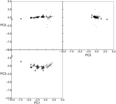
Figure 5: Principal planes for superclusters. PCA with the morphological parameters. Open circles: high-luminosity superclusters with luminosity $L_{g}>400$ $10^{10}h^{-2}L_{\sun}$; grey dots: superclusters of lower luminosity.

Figure 5 presents the locations of superclusters in the principal planes, defined by the luminosity and morphological parameters of superclusters. The upper lefthand panel shows the distribution of superclusters in the principal plane PC1-PC2. Here both high- and low-luminosity superclusters form an elongated cloud with very small scatter. The scatter of positions of the high-luminosity superclusters in PC1-PC3 plane is greater. Again, the more luminous the supercluster, the higher the negative value of its first principal component. High values of PC1 (and the highest values of PC3) correspond to luminous superclusters with high values of clumpiness $V_{3}$ (Table LABEL:tab:pcamorf). Large scatter along the second principal component PC2 in principal planes correspond to superclusters with high values of the shape parameter $K_{1}/K_{2}$. These are poor superclusters of “spider” morphology, for which the shape parameter is not well defined (Einasto et al. 2011a). We see that the luminosity and the morphological parameters of superclusters also define a fundamental plane for superclusters, where the physical and morphological properties are combined.

4.3 Scaling relations for superclusters and the fundamental plane

Table 6: Results of principal component analysis for luminosity, diameters, and shapefinders.

(1)	(2)	(3)	(4)
	PC1	PC2	PC3
$\log(L_{g})$	-0.5713	0.7905	-0.2205
$K1D$	-0.5833	-0.2020	0.7867
$K2D$	-0.5773	-0.5781	-0.5765
	Importance of components
	PC1	PC2	PC3
St.deviation	1.696	0.308	0.165
Prop.Variance	0.959	0.031	0.009
Cum.Proportion	0.959	0.990	1.000

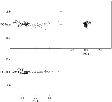
Figure 6: Principal planes for superclusters. PCA for the luminosity, diameter, and shapefinders as described in the text. Open circles: high-luminosity superclusters with luminosity $L_{g}>400$ $10^{10}h^{-2}L_{\sun}$, grey dots: superclusters of lower luminosity.

The results of the PCA suggest that the first two principal components define the fundamental plane for superclusters. This motivates us to find the scaling relations between the supercluster parameters. The scaling relations have earlier been found between the properties of galaxies, of groups of galaxies and of dark matter haloes (Faber & Jackson 1976; Tully & Fisher 1977; Kormendy 1977; Efstathiou & Fall 1984; Djorgovski & Davis 1987; Dressler et al. 1987; Schaeffer et al. 1993; Adami et al. 1998; Lanzoni et al. 2004; D’Onofrio et al. 2008; Woo et al. 2008; Araya-Melo et al. 2009b, and references therein).

For scaling relations we use Eq. (4) and perform the PCA for the parameters $\log(L_{g})$, $(1-K_{1})\cdot\log(Diameter)$ and $(1-K_{2})\cdot\log(Diameter)$. This set combines the easily detectable diameter of superclusters, and morphological parameters $K_{1}$ and $K_{2}$, which characterise the sizes and the shapes of superclusters, with the total luminosity of superclusters. For low values of shapefinders, $(1-K_{1})$ and $(1-K_{2})$ are less noisy than $K_{1}$ and $K_{2}$ (Einasto et al. 2011a).

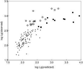
Figure 7: $L_{g{\mathrm{(observed)}}}$ vs. $L_{g{\mathrm{(predicted)}}}$, in units of $10^{10}h^{-2}L_{\sun}$. Open circles denote high-luminosity superclusters with the luminosity $L_{g}>400$ $10^{10}h^{-2}L_{\sun}$ and the shape parameter $K_{1}/K_{2}>0.5$ (less elongated superclusters), filled squares denote high-luminosity superclusters with the shape parameter $K_{1}/K_{2}<0.5$ (more elongated superclusters), grey dots denote superclusters of lower luminosity.

Table LABEL:tab:pca3scale and Fig. 6 present the principal components and principal planes of superclusters. Table LABEL:tab:pca3scale shows that the first two principal components account for 99% of the total variance of the parameters. The highest positive values of PC3 in Fig. 6 come from high-luminosity, very elongated superclusters. The values of PC3 for superclusters SCl 061 and SCl 094 were much higher than for other superclusters, therefore we excluded them from the calculations as outliers. These are the richest, most luminous, and most elongated systems with the largest clumpiness in our sample (Table LABEL:tab:basicscl and Einasto et al. 2011a). The supercluster SCl 061 is the richest member of the Sloan Great Wall, an exceptional system in the nearby universe (Einasto et al. 2011b; Sheth & Diaferio 2011). The supercluster SCl 094 (the Corona Borealis supercluster) is the richest system in the dominant supercluster plane (Einasto et al. 2011a). This system has been studied by Small et al. (1998); look also at the references in Einasto et al. (2011a).

Equation (5) and Fig. 7 show the resulting scaling relation.

$$\log(L_{g})=(5.11K_{2}-5.87K_{1}-0.76)\cdot\log(D)+1.29,$$ (5)

where $D$ denotes diameter. The standard deviation for the relation $sd=0.414$. Most of the scatter comes from the parameters of luminous superclusters, for them $sd=0.507$, for low-luminosity superclusters $sd=0.183$.

In Fig. 7 we denote the high-luminosity superclusters with different symbols, according to their shape parameter. Figure 7 shows that more elongated and less elongated high-luminosity superclusters populate the $L_{g{\mathrm{(observed)}}}$-$L_{g{\mathrm{(predicted)}}}$ plane differently. This suggests that luminous superclusters can be divided into two populations according to their shapes. Our calculations show that there is no such difference for low-luminosity superclusters. The differences between the observed and predicted luminosity are the largest for five systems with the highest predicted luminosity in Fig. 7. These are very elongated luminous superclusters in the sample, systems of (multibranching) filament morphology, SCl 064, SCl 189, SCl 336, and SCl 474, and a multispider SCl 530 (for morphological classification of superclusters we refer to Einasto et al. 2011a).

Next we derived the scaling relations separately for more elongated and less elongated high-luminosity superclusters (correspondingly, Eq. (6) and Eq. (7)), and for all low-luminosity superclusters (Eq. (8)):

$$\log(L_{g})=(0.22K_{2}-1.67K_{1}+1.45)\cdot\log(D)+0.69$$ (6)

$$\log(L_{g})=(3.45K_{2}-3.95K_{1}+0.50)\cdot\log(D)+2.09$$ (7)

$$\log(L_{g})=(63.80K_{2}-62.28K_{1}-1.52)\cdot\log(D)+3.81$$ (8)

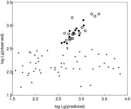
Figure 8: $L_{g{\mathrm{(observed)}}}$ vs. $L_{g{\mathrm{(predicted)}}}$, in units of $10^{10}h^{-2}L_{\sun}$. Open circles denote high-luminosity superclusters with the luminosity $L_{g}>400$ $10^{10}h^{-2}L_{\sun}$ and the shape parameter $K_{1}/K_{2}>0.5$ (less elongated superclusters), squares denote high-luminosity superclusters with the luminosity $L_{g}>400$ $10^{10}h^{-2}L_{\sun}$ and the shape parameter $K_{1}/K_{2}<0.5$ (more elongated superclusters), and grey dots denote superclusters of lower luminosity.

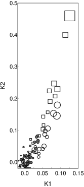
Figure 9: Shapefinders $K_{1}-K_{2}$ plane for superclusters. The size of symbols is proportional to the diameters of superclusters. Open circles denote high-luminosity superclusters with the luminosity $L_{g}>400$ $10^{10}h^{-2}L_{\sun}$ and the shape parameter $K_{1}/K_{2}>0.5$ (less elongated superclusters), squares denote high-luminosity superclusters with the luminosity $L_{g}>400$ $10^{10}h^{-2}L_{\sun}$ and the shape parameter $K_{1}/K_{2}<0.5$ (more elongated superclusters), grey filled circles denote superclusters of lower luminosity.

Figure 8 demonstrates the observed vs. predicted luminosity of superclusters found with these relations. Now luminosities of high-luminosity superclusters are recovered well, with a very small scatter ($sd=0.16$ and $sd=0.22$ for more elongated and less elongated superclusters). Interestingly, this figure shows the absence of the correlation between the observed and predicted luminosity for low-luminosity superclusters. To understand this, we plot in Fig. 9 the shapefinders $K_{1}-K_{2}$ plane for superclusters where the size of symbols is proportional to the diameters of superclusters. Here the values of shapefinders for high-luminosity superclusters are correlated, and these superclusters also have larger sizes. Most low-luminosity superclusters have very low, uncorrelated values of shapefinders (both $K_{1}$ and $K_{2}$ $<0.025$). For the smallest systems they are even negative. An example of such a system is the Virgo supercluster (Einasto et al. 2007e). The results of the PCA show that, while pairwise correlations between the luminosity and other parameters in Table LABEL:tab:rank are strong, the correlations between several parameters (diameters, shapefinders, and luminosities for most of low-luminosity superclusters) are almost absent, and so the scaling relation for them cannot be derived. Correlation between the observed and predicted luminosity for low-luminosity superclusters in Fig. 7 comes from the high-luminosity superclusters and from the low-luminosity superclusters with the shape parameters $K_{1}$ and $K_{2}$ $>0.025$.

5 Selection effects

The main selection effect in our study comes from the use of a flux-limited sample of galaxies to determine the luminosity density field and superclusters. To have luminosity-dependent selection effects as small as possible, we used data about galaxies and galaxy systems from a distance interval 90 – 320 $h^{-1}$ Mpc, in which these effects are the least (we refer to T10 for details). We showed above that the parameters of superclusters (except the number of galaxies) do not correlate with distance, which shows that the distant-dependent selection effects are correctly taken into account when generating the supercluster catalogue.

If the number of cells used to define superclusters is too small then the supercluster catalogue may include objects that cannot be considered as real superclusters. Moreover, the detection of the shape parameter becomes unreliable. If the shape parameter is determined using the inertia tensor method then superclusters have to be defined using at least eight members (Kolokotronis et al. 2001). In our study we determine shapefinders with Minkowski functionals, and the minimum number of cells for defining superclusters is 64 (Appendix A). We analysed systems in a distance interval where the selection effects are small. Even the poorest systems contain at least 25 to 30 galaxies and several groups of galaxies. Therefore the detection of the shape parameter may only be affected weakly by the selection effects except for the poorest systems of “spider” morphology for which the shapefinders may be noisy. We note that Costa-Duarte et al. (2011) include systems with at least ten member galaxies in their supercluster catalogue to study of the shape parameter of superclusters.

Another selection effect comes from the choice of the threshold density to determine superclusters. At the density level used in the present paper ($D=5.0)$, rich superclusters do not percolate yet. If we use a lower threshold density, new galaxies are added to superclusters, and some superclusters may join to form huge systems. At a higher density level, galaxies in the outskirts of the superclusters no longer belong to superclusters, and superclusters become poorer and smaller.

Table 7: Results of the principal component analysis for the threshold density level $D=5.5$.

(1)	(2)	(3)	(4)	(5)	(6)
	PC1	PC2	PC3	PC4	PC5
log$N_{\mbox{gal}}$	-0.437	0.085	0.889	-0.082	0.052
log$L_{g}$	-0.460	0.093	-0.146	0.854	-0.166
log$Diameter$	-0.447	0.523	-0.282	-0.443	-0.498
log$Volume$	-0.461	0.094	-0.298	-0.150	0.816
log$D_{peak}$	-0.428	-0.837	-0.136	-0.208	-0.233
Importance of components
	PC1	PC2	PC3	PC4	PC5
St.deviation	2.127	0.484	0.406	0.214	0.172
Prop.Variance	0.904	0.046	0.033	0.009	0.005
Cum.Proportion	0.904	0.951	0.984	0.994	1.000

Table 8: Results of the Spearman’s rank correlation test for the threshold density level $D=5.5$.

(1)	(2)	(3)
Parameters	$r$	$p$
$\log(L_{g})$ vs. $\log(N_{\mbox{gal}})$	0.85	$<2.2e-16$
$\log(L_{g})$ vs. $\log(Diameter)$	0.94	$<2.2e-16$
$\log(L_{g})$ vs. $\log(Volume)$	0.98	$<2.2e-16$
$\log(L_{g})$ vs. $\log(D_{\mbox{peak}})$	0.94	$<2.2e-16$

To see the sensitivity of the PCA results to the small differences in the choice of the threshold density, we compared the results of the PCA for superclusters chosen at higher and lower threshold density levels. As an example we show in Table LABEL:tab:pca55 the coefficients of the principal components for the superclusters chosen at the threshold density level $D=5.5$. At this density level, Luparello et al. (2011) determined superclusters in the SDSS-DR7 for volume-limited samples of galaxies. We used flux-limited samples, thus the density levels cannot be compared directly, but we can still choose this level for the present test. Table LABEL:tab:rank55 shows the results of the Spearman’s correlation test for this density level. The comparison with Tables LABEL:tab:pca90 and  LABEL:tab:rank shows that the coefficients are almost the same. Therefore the results of the correlation test and the PCA are not very sensitive to the choise of the density level.

6 Discussion and conclusions

We studied the properties of superclusters drawn from the SDSS DR7 using the principal component analysis and Spearman’s correlation test. Several earlier studies have shown that the properties of superclusters are correlated (see the references in Sect. 1). However, it is surprising that the correlations between the various properties of superclusters are so tight. The first two principal components account for most of the variance in the data. Different physical parameters (the luminosity, volume, and diameter) and the morphological parameters (the clumpiness and the shape parameters) are almost equally important in shaping the properties of superclusters. This suggests that superclusters, as described by their overall physical and morphological properties and by their inner morphology and peak density, are objects that can be described with a few parameters. We derived the scaling relation for superclusters in which we combine their luminosities, diameters, and shapefinders.

We saw in Fig. 7 that more elongated and less elongated high-luminosity superclusters populate the $L_{g(observed)}$-$L_{g(predicted)}$ plane differently. This suggests that luminous superclusters can be divided into two populations according to their shapes – more elongated systems with the shape parameter $K_{1}/K_{2}<0.5$ and less elongated ones with $K_{1}/K_{2}>0.5$. Einasto et al. (2011a) got a similar result using multidimensional normal mixture modelling. It is remarkable that two different multivariate methods reveal information about the data in such good agreement. However, there are few high-luminosity superclusters in our sample. There are 14 systems with the shape parameter $K_{1}/K_{2}<0.5$ among them, and 17 systems with $K_{1}/K_{2}>0.5$. A larger sample of superclusters has to be analysed to confirm this result.

Parameters used to characterise superclusters in the present study do not reflect all the properties of superclusters. For example, rich superclusters contain high-density cores that may contain merging X-ray clusters and may be collapsing (Small et al. 1998; Bardelli et al. 2000; Einasto et al. 2001; Rose et al. 2002; Einasto et al. 2007c, 2008). A supercluster environment with a wide range of densities affects the properties of galaxies, groups, and clusters located there (Einasto et al. 2003b; Plionis 2004; Wolf et al. 2005; Haines et al. 2006; Einasto et al. 2007d; Porter et al. 2008; Tempel et al. 2009; Fleenor & Johnston-Hollitt 2010; Tempel et al. 2011; Einasto et al. 2011b). Einasto et al. (2011b) showed that the dynamical evolution of one of the richest superclusters in the Sloan Great Wall (SCL 111, SCl 024 in L10 catalogue) is almost finished, while the richest member of the Wall, SCl 126 (SCl 061) is still dynamically active. Therefore our results reflect only certain aspects of the properties of superclusters.

Systems of galaxies determined in the SDSS have been studied by a number of authors (Pandey & Bharadwaj 2005; Gott et al. 2005; Park et al. 2005; Pandey & Bharadwaj 2006; Gott et al. 2008; Pandey & Bharadwaj 2008; Kitaura et al. 2009; Choi et al. 2010; Sousbie et al. 2011; Einasto et al. 2011b, a; Sheth & Diaferio 2011; Pimbblet et al. 2011; Platen et al. 2011). The overall shapes of superclusters have been described by the shape parameters or approximated by triaxial ellipses (Jaaniste et al. 1998; Basilakos et al. 2001; Kolokotronis et al. 2002; Basilakos 2003; Einasto et al. 2007a, 2011b, 2011a; Costa-Duarte et al. 2011; Luparello et al. 2011). These studies showed that elongated, prolate structures dominate among superclusters. The results obtained using the moments of inertia tensor (Basilakos et al. 2001; Basilakos 2003) or the Minkowski functionals are in a good agreement (see also Einasto et al. 2007e, 2011a). In addition, Basilakos et al. (2006) analysed correlations between supercluster properties from simulations and find that the amplitude of the supercluster - cluster alignment increases (weakly) with superclusters filamentarity.

The properties of superclusters are determined by their formation and evolution. Kolokotronis et al. (2002) show that the shapes of superclusters agree better with a $\Lambda$CDM model than with a $\tau$CDM model. Also Luparello et al. (2011) found that the shapes of observed superclusters agree with those in the $\Lambda$CDM model. In the $\Lambda$CDM concordance cosmological model, the matter density $\Omega_{\mathrm{m}}$ dominated in the early universe and the structures formed by hierarhical clustering driven by gravity. As the universe expands, the average matter density decreases. At a certain epoch, the dark energy density $\Omega_{\mathrm{\Lambda}}$ became higher than the matter density, and the universe started to expand acceleratingly. Simulations of the evolution and the future of the structure in an accelerating universe show the freezing of the web – the large-scale evolution of structures slows down (Loeb 2002; Nagamine & Loeb 2003; Dünner et al. 2006; Hoffman et al. 2007; Krauss & Scherrer 2007, and references therein). Araya-Melo et al. (2009a) show that this affects the sizes, the shapes, and the inner structure of superclusters, and they become rounder, smaller, and their multiplicity decreases. According to our present results, this suggests that in the future superclusters become less elongated and the scatter in the scaling relation of superclusters may decrease.

Summarising, our study showed that

• The PCA and Spearman’s correlation test showed the absence of correlations between the physical properties of superclusters and their distance, therefore the distance-dependent selection effects were taken into account properly when generating supercluster catalogues.

• The correlations between the properties of superclusters are tight. Different physical parameters (the luminosity, the volume, and the diameter) and the morphological parameters (the clumpiness and the shapefinders) of superclusters are equally important in shaping the properties of superclusters.

• The first two principal components account for more than 90% of the variance of the supercluster properties and define the fundamental plane of superclusters. This suggests that superclusters can be described with a few physical and morphological parameters. We derived the scaling relation for superclusters using data about their luminosities, diameters, and shapefinders.

• Superclusters can be divided into two populations according to their luminosity, using the luminosity limit $L_{\mbox{g}}=400$ $10^{10}h^{-2}L_{\sun}$. In agreement with Einasto et al. (2011a), we find that high-luminosity superclusters can be divided into two sets: more elongated systems with the shape parameter $K_{1}/K_{2}<0.5$ and less elongated ones with $K_{1}/K_{2}>0.5$.

For our study we chose a small sample of superclusters least affected by selection effects. To understand the properties of superclusters better the next step is to study a large sample of superclusters and high-redshift superclusters. A few superclusters at very high redshifts have already been discovered (Nakata et al. 2005; Swinbank et al. 2007; Gal et al. 2008; Tanaka et al. 2009; Planck Collaboration et al. 2011; Schirmer et al. 2011). Deep surveys like the ALHAMBRA project (Moles et al. 2008) will provide us with data about (possible) very distant superclusters. We also need more simulations with various cosmologies to understand the evolution and the properties of superclusters in detail.

Appendix A Luminosity density field and superclusters

To calculate the luminosity density field, we calculate the luminosities of groups first. In flux-limited samples, galaxies outside the observational window remain unobserved. To take into account the luminosities of the galaxies that lie outside the sample limits also we multiply the observed galaxy luminosities by the weight $W_{d}$. The distance-dependent weight factor $W_{d}$ was calculated as

$$W_{d}={\frac{\int_{0}^{\infty}L\,n(L)\mathrm{d}L}{\int_{L_{1}}^{L_{2}}L\,n(L)\mathrm{d}L}},$$ (9)

where $L_{1,2}=L_{\sun}10^{0.4(M_{\sun}-M_{1,2})}$ are the luminosity limits of the observational window at a distance $d$, corresponding to the absolute magnitude limits of the window $M_{1}$ and $M_{2}$; we took $M_{\sun}=4.64$ mag in the $r$-band (Blanton & Roweis 2007). Due to their peculiar velocities, the distances of galaxies are somewhat uncertain; if the galaxy belongs to a group, we use the group distance to determine the weight factor.

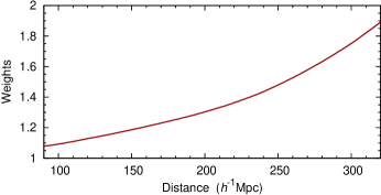
Figure 10: Weights used to correct for probable group members outside the observational luminosity window.

The luminosity weights for the groups of the SDSS DR7 in the distance interval 90 $h^{-1}$ Mpc$\geq D\leq$ 320 $h^{-1}$ Mpc are plotted as a function of the distance from the observer in Fig. 10. The mean weight is slightly higher than unity (about 1.4) within the sample limits. When the distance is greater, the weights increase owing to the absence of faint galaxies. Details of the calculations of weights are given also in Tempel et al. (2011). In the final flux-limited group catalogue, the richness of groups decreases rapidly at distances $D>320$ $h^{-1}$ Mpc due to selection effects (Tago et al. 2010; Einasto et al. 2011a). This is another reason to choose for our study superclusters from the distance interval 90 $h^{-1}$ Mpc $\leq D\leq$ 320 $h^{-1}$ Mpc  where the selection effects are weak. Even the poorest systems in our sample contain several groups of galaxies being real galaxy systems comparable to the Local supercluster.

To calculate a luminosity density field, we convert the spatial positions of galaxies $\mathbf{r}_{i}$ and their luminosities $L_{i}$ into spatial (luminosity) densities using kernel densities (Silverman 1986):

$$\rho(\mathbf{r})=\sum_{i}K\left(\mathbf{r}-\mathbf{r}_{i};a\right)L_{i},$$ (10)

where the sum is over all galaxies, and $K\left(\mathbf{r};a\right)$ is a kernel function of a width $a$. Good kernels for calculating densities on a spatial grid are generated by box splines $B_{J}$. Box splines are local and they are interpolating on a grid:

$$\sum_{i}B_{J}\left(x-i\right)=1,$$ (11)

for any $x$ and a small number of indices that give non-zero values for $B_{J}(x)$. We use the popular $B_{3}$ spline function:

$$B_{3}(x) = \left(|x-2|^{3}-4|x-1|^{3}+6|x|^{3}-\right.$$ (12)

$$\left.-4|x+1|^{3}+|x+2|^{3}\right)/12.$$

The (one-dimensional) $B_{3}$ box spline kernel $K_{B}^{(1)}$ of the width $a$ is defined as

$$K_{B}^{(1)}(x;a,\delta)=B_{3}(x/a)(\delta/a),$$ (13)

where $\delta$ is the grid step. This kernel differs from zero only in the interval $x\in[-2a,2a]$. It is close to a Gaussian with $\sigma=0.6$ in the region $x\in[-a,a]$, so its effective width is $2a$ (see, e.g., Saar 2009). The kernel preserves the interpolation property exactly for all values of $a$ and $\delta$, where the ratio $a/\delta$ is an integer. (This kernel can be used also if this ratio is not an integer, and $a\gg\delta$; the kernel sums to 1 in this case, too, with a very small error.) This means that if we apply this kernel to $N$ points on a one-dimensional grid, the sum of the densities over the grid is exactly $N$.

The three-dimensional kernel $K_{B}^{(3)}$ is given by the direct product of three one-dimensional kernels:

$$K_{B}^{(3)}(\mathbf{r};a,\delta)\equiv K_{3}^{(1)}(x;a,\delta)K_{3}^{(1)}(y;a,\delta)K_{3}^{(1)}(z;a,\delta),$$ (14)

where $\mathbf{r}\equiv\{x,y,z\}$. Although this is a direct product, it is isotropic to a good degree (Saar 2009).

In Einasto et al. (2007e) we compared the Epanechnikov, the Gaussian, and $B_{3}$ box spline kernels for calculating the density field. The Epanechnikov and the $B_{3}$ kernels are both compact, while the Gaussian kernel is infinite and has to be cut off at a fixed radius, which introduces an extra parameter. We also found that both the Epanechnikov and the $B_{3}$ kernels describe the overall shape of superclusters well, while the $B_{3}$ box spline kernel resolves the inner structure of superclusters better. This is why we used this kernel in the present study.

The densities were calculated on a cartesian grid based on the SDSS $\eta$, $\lambda$ coordinate system, as it allowed the most efficient fit of the galaxy sample cone into a brick. Using the rms velocity $\sigma_{v}$, translated into distance, and the rms projected radius $\sigma_{r}$ from the group catalogue (T10), we suppress the cluster finger redshift distortions. We divide the radial distances between the group galaxies and the group centre by the ratio of the rms sizes of the group finger:

$$d_{\mathrm{gal,f}}=d_{\mathrm{group}}+(d_{\mathrm{gal,i}}-d_{\mathrm{group}})\;\sigma_{\mathrm{r}}/\sigma_{\mathrm{v}}.$$ (15)

This removes the smudging effect the fingers have on the density field.

The grid coordinates are calculated according to Eq.2. We used an 1 $h^{-1}$ Mpc step grid and chose the kernel width $a=8$ $h^{-1}$ Mpc. This kernel differs from zero within the radius 16 $h^{-1}$ Mpc, but significantly so only inside the 8 $h^{-1}$ Mpc radius. As a lower limit for the volume of superclusters we used the value $(a/2)$ $h^{-1}$ Mpc³ (64 grid cells). In this way we exclude small spurious density field objects which include almost no galaxies. Liivamägi et al. (2010) tested the method generating the superclusters from the Millenium simulations. This comparison showed that supercluster algorithms work well, and, in addition, the selection effects have been properly taken into account when generating a supercluster catalogue from flux-limited sample of galaxies.

Before extracting superclusters we apply the DR7 mask constructed by P. Arnalte-Mur (Martínez et al. 2009; Liivamägi et al. 2010) to the density field and convert densities into units of mean density. The mean density is defined as the average over all pixel values inside the mask. The mask is designed to follow the edges of the survey and the galaxy distribution inside the mask is assumed to be homogeneous.

Appendix B Minkowski functionals and shapefinders

The supercluster morphology is fully characterised by the four Minkowski functionals $V_{0}$–$V_{3}$. For a given surface the four Minkowski functionals (from the first to the fourth) are proportional to the enclosed volume $V$, the area of the surface $S$, the integrated mean curvature $C$, and the integrated Gaussian curvature $\chi$ (Sahni et al. 1998; Martínez & Saar 2002; Shandarin et al. 2004; Saar et al. 2007; Saar 2009).

With the first three Minkowski functionals, we calculate the dimensionless shapefinders $K_{1}$ (planarity) and $K_{2}$ (filamentarity) (Sahni et al. 1998; Shandarin et al. 2004). See also Basilakos et al. (2001), in this study the shapefinders were determined with the moments of inertia method. First we calculate the shapefinders $H_{1}$–$H_{3}$ with a combination of Minkowski functionals: $H_{1}=3V/S$ (thickness), $H_{2}=S/C$ (width), and $H_{3}=C/4\pi$ (length). Then we use the shapefinders $H_{1}$–$H_{3}$ to calculate two dimensionless shapefinders $K_{1}$ (planarity) and $K_{2}$ (filamentarity): $K_{1}=(H_{2}-H_{1})/(H_{2}+H_{1})$ and $K_{2}=(H_{3}-H_{2})/(H_{3}+H_{2})$. We characterise the overall shape of superclusters using planarity $K_{1}$ and filamentarity $K_{2}$, and their ratio, $K_{1}$/$K_{2}$ (the shape parameter).

The fourth Minkowski functional $V_{3}$, describes the topology of the surface and gives the number of isolated clumps, the number of void bubbles, and the number of tunnels (voids open from both sides) in the region (see, e.g. Saar et al. 2007). Morphologically the superclusters with low values of the fourth Minkowski functional $V_{3}$ can be described as simple spiders or simple filaments. High values of the fourth Minkowski functional $V_{3}$ suggest a complicated (clumpy) morphology of a supercluster, described as multispiders or multibranching filaments (Einasto et al. 2007e, 2011a).

Appendix C Data on luminous ($L_{g}>400$ $10^{10}h^{-2}L_{\sun})$ superclusters

Table 9: Data on luminous ($L_{g}>400$ $10^{10}h^{-2}L_{\sun})$ superclusters

(1)	(2)	(3)	(4)	(5)	(6)	(7)	(8)	(9)	(10)	(11)	(12)	(13)
ID	ID	$Distance$	$L_{\mbox{g}}$	$N_{\mbox{gal}}$	$Volume$	$Diameter$	$D_{\mbox{peak}}$	$V_{3}$	$K_{1}$	$K_{2}$	$K_{1}/K_{2}$	$ID_{E01}$
		Mpc/$h$	$10^{10}h^{-2}L_{\sun}$		$(h^{-1}\mathrm{Mpc})^{3}$	Mpc/$h$
1	239+027+009	264	1591.5	1038	8435	50	21.6	2	0.080	0.152	0.527	162
10	239+016+003	111	680.2	1463	3378	22	16.4	1	0.038	0.015	2.456	160
11	227+006+007	233	1476.0	1222	8065	35	16.7	4	0.053	0.049	1.081	154
24	184+003+007	230	1768.2	1469	10040	56	14.1	5	0.089	0.145	0.616	111
38	167+040+007	224	660.7	586	3243	22	13.8	2	0.023	0.040	0.593	95
55	173+014+008	242	1773.0	1306	9684	50	12.3	5	0.091	0.179	0.509	111
60	247+040+002	92	527.4	1335	2472	21	12.0	2	0.013	0.021	0.645	160
61	202-001+008	255	4315.3	3056	23475	106	12.9	13	0.126	0.459	0.274	126
64	250+027+010	301	1305.4	619	6058	55	12.6	4	0.091	0.229	0.399	164
87	215+048+007	213	477.8	445	2301	21	11.0	2	0.039	0.026	1.494
94	230+027+006	215	2263.4	1830	11256	54	11.1	8	0.113	0.399	0.284	158
129	170+053+010	309	526.7	223	2321	20	10.6	3	0.029	0.048	0.612
136	189+017+007	212	523.2	504	2590	20	10.9	2	0.027	0.030	0.925	271
152	230+005+010	301	907.5	423	4756	32	10.8	3	0.057	0.097	0.585	160
189	126+017+009	267	771.0	433	3063	43	9.5	4	0.070	0.190	0.372
195	134+038+009	280	487.9	273	2200	23	9.9	2	0.031	0.031	1.004
198	152-000+009	284	863.9	473	4448	38	9.7	4	0.050	0.103	0.490	82
223	187+008+008	268	703.7	462	3368	33	9.3	3	0.051	0.142	0.361	111
228	203+059+007	210	644.0	643	3361	31	9.5	2	0.040	0.040	0.992	133
327	170+000+010	302	419.8	205	1747	20	8.5	2	0.016	0.071	0.228
332	175+005+009	291	664.3	333	3128	27	8.2	3	0.062	0.078	0.788	106
336	172+054+007	207	1003.6	1005	4605	53	8.7	5	0.082	0.246	0.332	109
349	207+026+006	188	768.8	893	3942	42	8.8	4	0.064	0.105	0.610	138
350	230+008+003	105	436.3	955	1987	22	8.0	2	0.022	0.059	0.383	160
351	207+028+007	225	689.1	615	3292	32	8.7	4	0.056	0.086	0.647	138
366	217+020+010	300	763.4	353	3681	31	8.1	4	0.064	0.156	0.409	158
376	255+033+008	258	658.0	437	3097	27	8.6	4	0.050	0.041	1.228	167
474	133+029+008	251	612.6	389	2299	43	7.6	4	0.068	0.223	0.307	76
512	168+002+007	227	410.7	371	1658	26	7.5	3	0.040	0.082	0.490	91
530	192+062+010	306	790.3	333	3690	40	7.5	4	0.084	0.207	0.409
827	189+003+008	254	572.4	405	2238	30	6.7	4	0.052	0.116	0.450