Testing a Predictive Theoretical Model for the Mass Loss Rates of Cool Stars

Abstract

The basic mechanisms responsible for producing winds from cool, late-type stars are still largely unknown. We take inspiration from recent progress in understanding solar wind acceleration to develop a physically motivated model of the time-steady mass loss rates of cool main-sequence stars and evolved giants. This model follows the energy flux of magnetohydrodynamic turbulence from a subsurface convection zone to its eventual dissipation and escape through open magnetic flux tubes. We show how Alfvén waves and turbulence can produce winds in either a hot corona or a cool extended chromosphere, and we specify the conditions that determine whether or not coronal heating occurs. These models do not utilize arbitrary normalization factors, but instead predict the mass loss rate directly from a star’s fundamental properties. We take account of stellar magnetic activity by extending standard age-activity-rotation indicators to include the evolution of the filling factor of strong photospheric magnetic fields. We compared the predicted mass loss rates with observed values for 47 stars and found significantly better agreement than was obtained from the popular scaling laws of Reimers, Schröder, and Cuntz. The algorithm used to compute cool-star mass loss rates is provided as a self-contained and efficient computer code. We anticipate that the results from this kind of model can be incorporated straightforwardly into stellar evolution calculations and population synthesis techniques.

1. Introduction

All stars are believed to possess expanding outer atmospheres known as stellar winds. Continual mass loss has a significant impact on the evolution of the stars themselves, on surrounding planetary systems, and on the evolution of gas and dust in galaxies (see reviews by Dupree, 1986; Lamers & Cassinelli, 1999; Puls et al., 2008). For example, the Sun’s own mass loss was probably an important factor in the early erosion of atmospheres from the inner planets of our solar system (e.g., Wood, 2006; Güdel, 2007). On the opposite end of the distance scale, a better understanding of the winds from supergiant stars is leading to new ways of using them as “standard candles” to measure the distances to other galaxies (Kudritzki, 2010). By studying the physical mechanisms that drive stellar winds, as well as their interaction with processes occurring inside the stars (convection, pulsation, rotation, and magnetic fields), we are able to make better quantitative predictions about a wide range of astrophysical environments.

Over the last half-century, there has been a great deal of research into possible mechanisms for driving stellar winds on the “cool side” of the Hertzsprung-Russell diagram; i.e., effective temperatures less than about 8000 K (Holzer & Axford, 1970; Hartmann & MacGregor, 1980; Hearn, 1988; Lafon & Berruyer, 1991; Mullan, 1996; Willson, 2000; Holzwarth & Jardine, 2007). Despite this work, there is still no agreement about the fundamental mechanisms responsible for producing these winds. Many studies of stellar evolution use approximate prescriptions for mass loss that do not depend on a true physical model of how the outflow is produced (Reimers, 1975; Leitherer, 2010). Observational validation of models is made difficult because mass loss rates similar to that of the solar wind ($\dot{M}\sim 10^{-14}$ $M_{\odot}$ yr^-1) tend to be too low to be detectable in most observational diagnostics.

Fortunately, there has been a great deal of recent progress toward identifying and characterizing the processes that produce our own Sun’s wind. Self-consistent models of turbulence-driven coronal heating and solar wind acceleration have begun to succeed in reproducing a wide range of observations without the need for ad hoc free parameters (e.g., Suzuki, 2006; Cranmer et al., 2007; Rappazzo et al., 2008; Verdini et al., 2010; Bingert & Peter, 2011; van Ballegooijen et al., 2011). This progress on the solar front provides a fruitful opportunity to better understand the fundamental physics of coronal heating and wind acceleration in other kinds of stars.

The goal of this paper is to construct self-consistent physical models of cool-star wind acceleration. These models predict stellar mass loss rates without the need for observationally constrained normalization parameters, artificial heating functions, or imposed damping lengths for waves. We aim to describe time-steady mass outflows from main-sequence stars with solar-type coronae and from giants with cooler outer atmospheres. In principle, then, these models cross the well-known dividing line (Linsky & Haisch, 1979) between stars with and without X-ray emission. However, there are several types of late-type stellar winds that our models do not attempt to explain: (1) Highly evolved supergiants and asymptotic giant branch (AGB) stars presumably have winds driven by radiation pressure on dust grains (Lafon & Berruyer, 1991; Höfner, 2011) and/or strong radial pulsations (Willson, 2000). (2) T Tauri stars have polar outflows that may be energized by magnetospheric streams of infalling gas from their accretion disks (e.g., Cranmer, 2008). (3) Blue horizontal branch stars may have line-driven stellar winds similar to those of O, B, and A type stars (Vink & Cassisi, 2002).

The remainder of this paper is organized as follows. In Section 2 we outline the relevant properties of Alfvén waves and magnetohydrodynamic (MHD) turbulence that we expect to find in cool-star atmospheres. Section 3 presents derivations of two complementary models of mass loss for stars with and without hot coronae, and also describes how we estimate the total mass loss due to both gas pressure and wave pressure gradients. Section 4 summarizes how we determine the level of magnetic activity in a star based on its rotation rate and other fundamental parameters. We then give the resulting predictions for mass loss rates of cool stars in Section 5 and compare the predictions with existing observational constraints. Finally, Section 6 concludes this paper with a brief summary of the major results, a discussion of some of the broader implications of this work, and suggestions for future improvements.

2. Alfvén Waves in Stellar Atmospheres

For several decades, MHD fluctuations have been studied as likely sources of energy and momentum for accelerating winds from cool stars (see, e.g., Hollweg, 1978; Hartmann & MacGregor, 1980; DeCampli, 1981; Wang & Sheeley, 1991; Airapetian et al., 2000; Falceta-Gonçalves et al., 2006; Suzuki, 2007). Specifically, the dissipation of MHD turbulence as a potential source of heating for the solar wind goes back to Coleman (1968) and Jokipii & Davis (1969). Despite the fact that other sources of heating and acceleration may exist, we choose to explore how much can be explained by restricting ourselves to just this one set of processes. The ideas outlined here will be applied to both the “hot” and “cold” models for mass loss described in Section 3.

2.1. Setting the Photospheric Properties

We begin with five fundamental parameters that are assumed to determine (nearly) all of the other relevant properties of a star: mass $M_{\ast}$, radius $R_{\ast}$, bolometric luminosity $L_{\ast}$, rotation period $P_{\rm rot}$, and metallicity. We also assume that the star’s iron abundance, expressed logarithmically with respect to hydrogen, is a good enough proxy for the abundances of other elements heavier than helium; i.e., [Fe/H] $\approx\log(Z/Z_{\odot})$. For spherical stars, the effective temperature $T_{\rm eff}$ and surface gravity $g$ are calculated straightforwardly from

$$\sigma T_{\rm eff}^{4}\,=\,\frac{L_{\ast}}{4\pi R_{\ast}^{2}}\,\,,\,\,\,\,g\,=\,\frac{GM_{\ast}}{R_{\ast}^{2}}\,\,,$$ (1)

where $\sigma$ is the Stefan-Boltzmann constant and $G$ is the Newtonian gravitation constant.

We need to know the mass density in the stellar photosphere $\rho_{\ast}$ in order to specify the properties of MHD waves at that height. The density was computed from the criterion that the Rosseland mean optical depth should have a value of $2/3$ in the photosphere. We used the AESOPUS opacity database, which is a tabulation of the Rosseland mean opacity $\kappa_{\rm R}$ as a function of temperature, density, and metallicity (see Marigo & Aringer, 2009). An approximate expression for the Rosseland optical depth $\tau_{\rm R}$ in the photosphere,

$$\tau_{\rm R}\,=\,\kappa_{\rm R}\rho_{\ast}H_{\ast}\,=\,2/3\,\,,$$ (2)

was solved for $\rho_{\ast}$, where $H_{\ast}$ is the photospheric value of the density scale height (see below). We used straightforward linear interpolation to locate the relevant solutions for $\rho_{\ast}$ as a function of $T_{\rm eff}$, $g$, and [Fe/H].

Figure 1(a) shows how the photospheric density varies as a function of $T_{\rm eff}$ and $\log\,g$ under the assumption of solar metallicity ([Fe/H] $=0$). For context we also show the location of the zero-age main sequence (ZAMS) from the models of Girardi et al. (2000), as well as a post-main-sequence evolutionary track for a 1 $M_{\odot}$ star from the BaSTI model database (Pietrinferni et al., 2004).

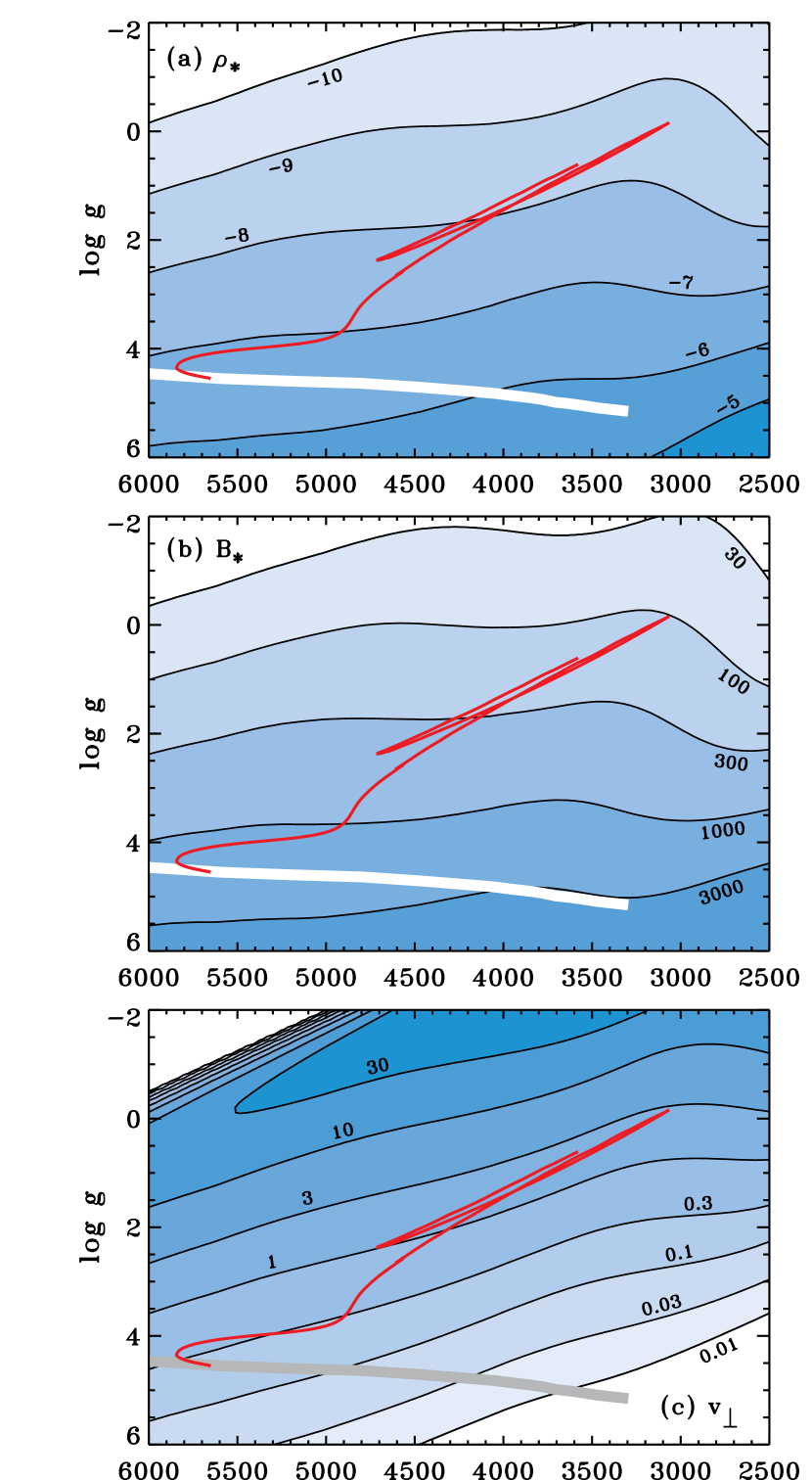
Figure 1.— Derived photospheric parameters shown as a function of both $T_{\rm eff}$ and $\log\,g$. Contour labels denote (a) base-10 logarithm of mass density $\rho_{\ast}$ in g cm^-3, (b) magnetic field strength $B_{\ast}$ in G, and (c) Alfvén wave amplitude $v_{\perp\ast}$ in km s^-1. Also shown is a post-main-sequence evolutionary track for a 1 $M_{\odot}$ star (red curves) and the location of the ZAMS (white and gray curves).

We used the 2005 release of OPAL plasma equations of state (see also Rogers & Nayfonov, 2002) to estimate the mean atomic weight $\mu$ in a partially ionized photosphere. For the range of parameters appropriate for cool stars, we found that $\mu$ is primarily sensitive to $T_{\rm eff}$, and not to gravity or metallicity, so we produced a single parameter fit,

$$\mu\,\approx\,\frac{7}{4}+\frac{1}{2}\tanh\left(\frac{3500-T_{\rm eff}}{600}\right)$$ (3)

where $T_{\rm eff}$ is expressed in K. Other quantities that will be needed later include the photospheric density scale height, which is given by

$$H_{\ast}\,=\,\frac{k_{\rm B}T_{\rm eff}}{\mu m_{\rm H}g}$$ (4)

where $k_{\rm B}$ is Boltzmann’s constant and $m_{\rm H}$ is the mass of a hydrogen atom. We also need to compute the equipartition magnetic field strength,

$$B_{\rm eq}\,=\,\sqrt{8\pi P_{\ast}}\,=\,\sqrt{\frac{8\pi\rho_{\ast}k_{\rm B}T_{\rm eff}}{\mu m_{\rm H}}}\,\,,$$ (5)

where $P_{\ast}$ is the photospheric gas pressure. Because $T_{\rm eff}$ and $\mu$ do not vary over many orders of magnitude, it is roughly the case that $B_{\rm eq}\propto\rho_{\ast}^{1/2}$. However, in all calculations below we compute $B_{\rm eq}$ fully from Equation (5). In Section 4 we describe observations that show the photospheric magnetic field strength $B_{\ast}$ is roughly linearly proportional to $B_{\rm eq}$ for many stars. The measurements determine the constant of proportionality, and we use

$$B_{\ast}\,=\,1.13\,B_{\rm eq}$$ (6)

in the remainder of this paper. Figure 1(b) shows $B_{\ast}$ as a function of $T_{\rm eff}$ and $\log\,g$.

We consider MHD waves that are driven by turbulent convective motions in the stellar interior. The original models of wave generation from turbulence (e.g., Lighthill, 1952; Proudman, 1952; Stein, 1967) dealt mainly with acoustic waves in an unmagnetized medium. More recently, however, it has been shown that when a stellar atmosphere is filled with magnetic flux tubes, the dominant carrier of wave energy should be transverse kink-mode oscillations (Musielak & Ulmschneider, 2002a). When the magnetic flux tubes extend above the stellar surface and expand to fill the volume, the kink-mode waves become shear Alfvén waves (see Cranmer & van Ballegooijen, 2005).

We utilize the model results of Musielak & Ulmschneider (2002a) to estimate the flux of energy in kink/Alfvén waves in stellar photospheres. For simplicity, we used only the simulations of Musielak & Ulmschneider (2002a) with their standard parameter choices: a mixing length parameter of $\alpha=2$ and a constant magnetic field strength that is 0.85 times the equipartition field strength. Our analytic fit to the results shown in their Figure 8 is

$$F_{\rm A\ast}\,=\,F_{0}\left(\frac{T_{\rm eff}}{T_{0}}\right)^{\varepsilon}\exp\left[-\left(\frac{T_{\rm eff}}{T_{0}}\right)^{25}\right]$$ (7)

where the dependence on $\tilde{g}=\log\,g$ is given by

$$\frac{F_{0}}{10^{9}\,\,\mbox{erg}\,\,\,\mbox{cm}^{-2}\,\,\,\mbox{s}^{-1}}\,=\,5.724\,\,\exp\left(-\frac{\tilde{g}}{11.48}\right)\,\,,$$ (8)

$$\frac{T_{0}}{1000\,\,\mbox{K}}\,=\,5.624+0.6002\,\tilde{g}\,\,,$$ (9)

$$\varepsilon\,=\,6.774+0.5057\,\tilde{g}\,\,.$$ (10)

These fits are similar in form to those given by Fawzy & Cuntz (2011) for longitudinal MHD waves. Figure 2 shows a comparison between the above fitting formula and the plotted results of Musielak & Ulmschneider (2002a) for $\log\,g=3$, 4, and 5. The behavior of $F_{\rm A\ast}$ for lower values of $\log\,g$ was not given by Musielak & Ulmschneider (2002a), but similar results were found for a wider range of gravities by Ulmschneider et al. (1996) for acoustic waves.

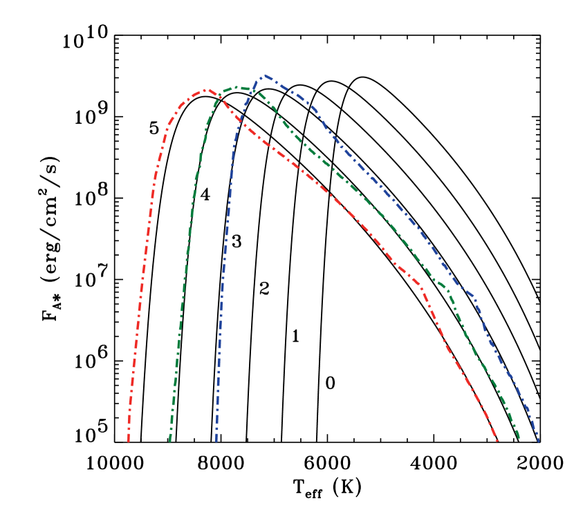
Figure 2.— Comparison between the Musielak & Ulmschneider (2002a) numerical models (dot-dashed curves) and analytic fits (solid curves) for photospheric transverse wave energy fluxes $F_{\rm A\ast}$ as a function of effective temperature and photospheric gravity. Numerical labels denote $\log\,g$ for each curve.

We used the kink-mode energy flux to determine the transverse velocity amplitude $v_{\perp}$ of Alfvén waves in the photosphere. The flux is defined as

$$F_{\rm A\ast}\,=\,\rho_{\ast}v_{\perp\ast}^{2}V_{{\rm A}\ast}$$ (11)

with $V_{{\rm A}\ast}=B_{\ast}/(4\pi\rho_{\ast})^{1/2}$ being the photospheric Alfvén speed. The above expression is not exact for waves undergoing strong reflection (see, e.g., Heinemann & Olbert, 1980), but it ends up giving a similar prediction for the height variation of $v_{\perp}$ in the corona that would come from a more accurate non-WKB model (Cranmer & van Ballegooijen, 2005). Figure 1(c) shows how $v_{\perp\ast}$ varies as a function of $T_{\rm eff}$ and $\log\,g$ for solar metallicity stars.

For the well-observed case of the Sun, we know that most of the photospheric magnetic field is concentrated into small (100–200 km diameter) flux tubes concentrated in the intergranular downflow lanes (Solanki, 1993; Berger & Title, 2001). The field strength in these tubes is close to equipartition, with $B_{\ast}\approx 1400$ G. However, these flux tubes have a filling factor $f_{\ast}$ in the photosphere of about 0.1% to 1%, so the spatially averaged magnetic flux density $B_{\ast}f_{\ast}$ is only of order 1–10 G (Schrijver & Harvey, 1989).

2.2. Radial Evolution of Waves and Turbulence

Figure 3 illustrates the stellar magnetic field geometry that we assume to exist above the surface of a cool star. Flux tubes that are open to the stellar wind have a cross-sectional area $A(r)$ that expands monotonically with increasing radial distance $r$ from the star. The condition $\nabla\cdot{\bf B}=0$ demands that the product of $A$ and the magnetic field strength $B$ remains constant. Thus, $B(r)$ inside a flux tube decreases monotonically, from its photospheric value of $B_{\ast}$, with increasing distance. We normalize $A$ such that at a given distance the total stellar surface area covered by open flux tubes is defined to be

$$A\,=\,4\pi r^{2}f\,\,.$$ (12)

The dimensionless filling factor $f$ tends to increase with height to an asymptotic value of 1 as $r\rightarrow\infty$ (see also Cuntz et al., 1999), but its increase is not necessarily monotonic. We do not explicitly consider the properties of closed magnetic “loops” on the stellar surface, but the radial variation of $f(r)$ takes into account their presence.

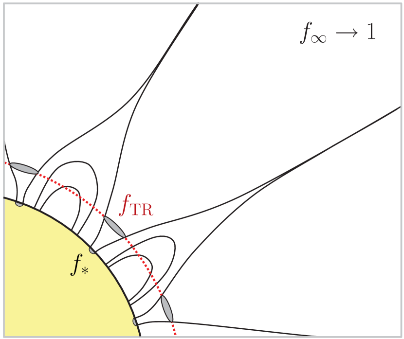
Figure 3.— Summary illustration of flux tube expansion on a representative cool star. The filling factor (for open magnetic flux tubes) grows from $f_{\ast}$ in the photosphere to $f_{\rm TR}$ at the transition region, and to an asymptotic value $f_{\infty}\rightarrow 1$ at large distances. The dimensions in this sketch are not drawn to scale.

For each star, we intend to specify $f_{\ast}$ on the basis of either direct measurements or empirical scaling relations. The model described in Section 3.1 also requires specifying the value of $f$ at the sharp transition region (TR) between the cool chromosphere and hot corona. We generally know that $f_{\ast}<f_{\rm TR}<1$, so in the absence of better information we will apply the assumption that that $f_{\rm TR}=f_{\ast}^{\theta}$, where $\theta$ is a dimensionless constant between 0 and 1. For the solar wind models of Cranmer et al. (2007) the exponent $\theta$ ranges between about 0.3 and 0.5.

Alfvén waves propagate up from the stellar photosphere, partially reflect back down toward the Sun, develop into strong MHD turbulence, and dissipate gradually (Velli et al., 1991; Matthaeus et al., 1999; Cranmer & van Ballegooijen, 2005). Temporarily ignoring the reflection and turbulent cascade, the overall energy balance of an Alfvén wave train is governed by the conservation of wave action. We define the flux of wave action $\tilde{S}$ as

$$\tilde{S}\,\equiv\,\rho v_{\perp}^{2}V_{\rm A}(1+M_{\rm A})^{2}A\,=\,\mbox{constant}$$ (13)

where $M_{\rm A}=u/V_{\rm A}$ is the Alfvén Mach number and $u$ is the radial outflow speed of the wind (see, e.g., Jacques, 1977; Tu & Marsch, 1995). Close to the stellar surface, where $M_{\rm A}\ll 1$, this condition is equivalent to energy flux conservation ($F_{\rm A}A=\mbox{constant}$). In any case, the constant value of $\tilde{S}$ in Equation (13) is known for each star because the conditions at the photosphere are known (and it is also valid to assume $M_{\rm A}\rightarrow 0$ there as well). The behavior of the wave amplitude as a function of density varies from $v_{\perp}\propto\rho^{-1/4}$ close to the star to $v_{\perp}\propto\rho^{+1/4}$ at larger distances.

The waves gradually lose energy due to turbulent dissipation, but for locations reasonably close to the stellar surface—e.g., the region shown in Figure 3—it is not a bad approximation to use the undamped form of wave action conservation to compute the radial dependence of $v_{\perp}$ (see Cranmer & van Ballegooijen, 2005). Wave damping gives rise to plasma heating, and we adopt a phenomenological heating rate that is consistent with the total energy flux that cascades from large to small eddies. This rate is constrained by the properties of the Alfvénic fluctuations at the largest scales, and it does not specify the exact kinetic means of dissipation once the energy reaches the smallest scales. Dimensionally, it is similar to the rate of cascading energy flux derived by von Kármán & Howarth (1938) for isotropic hydrodynamic turbulence. The volumetric heating rate is given by

$$Q\,=\,\frac{\tilde{\alpha}\rho v_{\perp}^{3}}{\lambda_{\perp}}$$ (14)

(Hollweg, 1986; Hossain et al., 1995; Zhou & Matthaeus, 1990; Matthaeus et al., 1999; Dmitruk et al., 2002). The dimensionless efficiency factor $\tilde{\alpha}$ depends on the local degree of wave reflection and is discussed further below. The perpendicular length scale $\lambda_{\perp}$ is an effective correlation length for the largest eddies in the turbulent cascade.

MHD turbulence occurs only when there exist counter-propagating Alfvén wave packets along a flux tube. The star naturally creates upward waves, and we assume that linear reflection gives rise to downward waves (Ferraro & Plumpton, 1958). We specify the ratio of downward to upward wave amplitudes by the effective reflection coefficient ${\cal R}$, and the efficiency factor $\tilde{\alpha}$ is given by

$$\tilde{\alpha}\,=\,\alpha_{0}\frac{{\cal R}(1+{\cal R})\sqrt{2}}{(1+{\cal R}^{2})^{3/2}}$$ (15)

(see, e.g., Cranmer et al., 2007). At the photospheric lower boundary, we assume total reflection with ${\cal R}=1$ and thus $\tilde{\alpha}=\alpha_{0}$. Higher in the stellar atmosphere, we use the low-frequency limiting expression of Cranmer (2010),

$${\cal R}\,\approx\,\frac{V_{\rm A}-u_{\infty}}{V_{\rm A}+u_{\infty}}\,\,,$$ (16)

where the wind’s terminal speed is $u_{\infty}$ and we also assume that $M_{\rm A}\ll 1$ in the atmosphere. This expression also assumes that the wind speed at the point where $M_{\rm A}=1$ (presumably far from the stellar surface) is roughly equal to $u_{\infty}$. We also set $\alpha_{0}=0.5$ based on the turbulent transport models of Breech et al. (2009).

3. Models for Mass Loss

In this section we present two complementary descriptions of cool-star mass loss that make use of the Alfvén wave properties discussed above. Supersonic winds can be driven by either gas pressure in a hot corona (Section 3.1) or wave pressure in a cool, extended chromosphere (Section 3.2). We first investigate each idea by assuming the other one is negligible, and then we explore how to incorporate both processes together (Section 3.3).

3.1. Hot Coronal Mass Loss

If the turbulent heating given by Equation (14) is sufficient to produce a hot ($T\gtrsim 10^{6}$ K) corona, then the plasma’s high gas pressure gradient may provide enough outward acceleration to produce a transition from a subsonic (bound) state near the star to a supersonic (outflowing) state at larger distances (Parker, 1958). In this section we estimate the mass loss rate $\dot{M}$ of such a gas-pressure-driven stellar wind.

We begin by computing $Q_{\ast}$ in the photosphere using $\rho_{\ast}$ and $v_{\perp\ast}$ in Equation (14). For the Sun, we have the observational constraint that $\lambda_{\perp\ast}$ must be about the size of the granular motions that jostle the flux tubes (i.e., roughly 100–1000 km). For other stars we can assume that the horizontal scale of granulation remains proportional to the photospheric pressure scale height (Robinson et al., 2004). Thus, we use

$$\lambda_{\perp\ast}\,=\,\lambda_{\perp\odot}\,\frac{H_{\ast}}{H_{\odot}}\,\,,$$ (17)

where $H_{\odot}=139$ km and the models of Cranmer & van Ballegooijen (2005) were used to set the solar normalization of the correlation length to $\lambda_{\perp\odot}=300$ km.

In the photosphere, we assume the turbulent heating is swamped by radiative gains and losses that are determined by the conditions of local thermodynamic equilibrium (LTE), and the temperature is set by those processes alone. At larger heights in the flux tube, the turbulent heating $Q$ begins to have an effect. We define the chromosphere as the region in which $Q$ is balanced by radiative losses. As one increases in height, however, the density drops to the point where radiative losses alone can no longer balance the imposed heating rate; this occurs at the sharp TR between chromosphere and corona. (See Section 3.2 for cases where this transition does not occur at all.)

In the region between the photosphere and the TR, we assume that the wind flow speed is sufficiently sub-Alfvénic such that $v_{\perp}\propto\rho^{-1/4}$. We also assume that $\lambda_{\perp}$ scales with the transverse size of the magnetic flux tube, so that $\lambda_{\perp}\propto A^{1/2}\propto B^{-1/2}$ (Hollweg, 1986). Thus, Equation (14) can be rewritten as

$$\frac{Q_{\rm TR}}{Q_{\ast}}\,=\,\frac{\tilde{\alpha}_{\rm TR}}{\tilde{\alpha}_{\ast}}\left(\frac{\rho_{\rm TR}}{\rho_{\ast}}\right)^{1/4}\left(\frac{B_{\rm TR}}{B_{\ast}}\right)^{1/2}$$ (18)

where $\tilde{\alpha}_{\ast}=0.5$ and all other photospheric quantities are assumed to be known. We also know that

$$\frac{B_{\rm TR}}{B_{\ast}}\,=\,\frac{f_{\ast}}{f_{\rm TR}}\,\approx\,f_{\ast}^{1-\theta}$$ (19)

where the last approximation holds if there is a universal relationship between $f_{\ast}$ and $f_{\rm TR}$ as speculated in Section 2.2 above.

Just below the TR, the heating is just barely balanced by radiative cooling. In the optically thin limit, radiative cooling behaves as $Q_{\rm cool}=-n^{2}\Lambda(T)$, where $n$ is the number density in the fully ionized TR region. Let us then assume that $Q_{\rm TR}=\max|Q_{\rm cool}|$, where

$$\max|Q_{\rm cool}|\,=\,\frac{\rho_{\rm TR}^{2}\Lambda_{\rm max}}{m_{\rm H}^{2}}\,\,.$$ (20)

The quantity $\Lambda_{\rm max}$ is the absolute maximum of the radiative loss curve $\Lambda(T)$, and it occurs roughly at $T_{\rm TR}=2\times 10^{5}$ K. The value of $\Lambda_{\rm max}$ depends on metallicity. To work out its dependence on $Z$, we computed a number of radiative loss curves for different metal abundances using version 4.2 of the CHIANTI atomic database (Young et al., 2003) with collisional ionization balance (Mazzotta et al., 1998). We started with a traditional (Grevesse & Sauval, 1998) solar abundance mixture ($Z/Z_{\odot}=1$) and then recomputed $\Lambda(T)$ by varying the metal abundance ratio $Z/Z_{\odot}$ between 0 and 10. We found that the maxima of the curves were fit well by the following parameterized function,

$$\frac{\Lambda_{\rm max}}{10^{-23}\,\mbox{erg}\,\,\mbox{cm}^{3}\,\,\mbox{s}^{-1}}\,\approx\,7.4+42\left(\frac{Z}{Z_{\odot}}\right)^{1.13}\,\,.$$ (21)

Other examples of the metallicity dependence of $\Lambda(T)$ have been given by, e.g., Boehringer & Hensler (1989) and Gnat & Sternberg (2007). We have ignored any possible differences between a star’s photospheric metal abundances and those in the low corona, although such differences have been measured in some cases (Testa, 2010).

With the above assumptions, we solve for the TR density,

$$\rho_{\rm TR}\,=\,\left[\frac{\tilde{\alpha}_{\rm TR}Q_{\ast}m_{\rm H}^{2}}{\tilde{\alpha}_{\ast}\rho_{\ast}^{1/4}\Lambda_{\rm max}}\right]^{4/7}{f_{\ast}}^{2(1-\theta)/7}$$ (22)

and we also derive the heating rate at the TR to be

$$Q_{\rm TR}\,=\,\left(\frac{\tilde{\alpha}_{\rm TR}Q_{\ast}}{\tilde{\alpha}_{\ast}}\right)^{8/7}\left(\frac{m_{\rm H}^{2}}{\rho_{\ast}^{2}\Lambda_{\rm max}}\right)^{1/7}{f_{\ast}}^{4(1-\theta)/7}\,\,.$$ (23)

A potential roadblock to solving Equations (22–23) is that we do not initially know the value of $\tilde{\alpha}_{\rm TR}$. This quantity depends on the reflection coefficient ${\cal R}$, which depends on the Alfvén speed $V_{\rm A}$ at the TR (see Equation (16)), which in turn depends on the unknown value of $\rho_{\rm TR}$. In practice, we solve these equations iteratively. We start with an initial estimate of ${\cal R}=0.5$, we compute $\tilde{\alpha}_{\rm TR}$, $\rho_{\rm TR}$, and $V_{\rm A}$ at the TR, and then we recompute ${\cal R}$ for the next iteration. In all cases the process converges to a self-consistent set of values (with a relative accuracy of $\sim 10^{-7}$) in no more than 20 iterations.

The mass loss rate of the stellar wind is determined by the heating rate $Q_{\rm TR}$ as well as other sources and sinks of energy at the TR. The general idea that the solar wind’s mass flux is set by the energy balance at the TR was first discussed by Hammer (1982). Hansteen & Leer (1995) worked out the basic scaling argument that is used below (see also Leer et al., 1982; Withbroe, 1988; Schwadron & McComas, 2003). In the low corona and wind, the time-steady equation of internal energy conservation is

$$\frac{1}{A}\frac{\partial}{\partial r}\left\{A\left[F_{\rm H}-F_{\rm cond}+\rho u\left(\frac{u^{2}}{2}-\frac{GM_{\ast}}{r}\right)\right]\right\}\,=\,0\,\,,$$ (24)

where $F_{\rm H}$ is the energy flux associated with the heating, $F_{\rm cond}$ is the energy flux transported by heat conduction along the field, and $u$ is the outflow speed. The term in braces is constant as a function of radius, so it is straightforward to equate its value at the TR to its asymptotic value at $r\rightarrow\infty$. The kinetic energy term proportional to $u^{2}$ is assumed to be negligibly small at the TR, but we assume it dominates the energy balance at large distances. Thus,

$$A_{\rm TR}\left(F_{\rm H,TR}-F_{\rm cond}\right)-(\rho uA)_{\rm TR}\frac{GM_{\ast}}{R_{\ast}}\,=\,(\rho uA)_{\infty}\frac{u_{\infty}^{2}}{2}\,\,,$$ (25)

where $F_{\rm H,TR}$ is the heat flux $F_{\rm H}$ at the TR, and we realize that the product $\rho uA$ is also constant via mass flux conservation. We also make the key assumption that $u_{\infty}=V_{\rm esc}=(2GM_{\ast}/R_{\ast})^{1/2}$, and thus we can write

$$\dot{M}\,\equiv\,\rho uA\,=\,\frac{4\pi R_{\ast}^{2}f_{\rm TR}}{V_{\rm esc}^{2}}\left(F_{\rm H,TR}-F_{\rm cond}\right)\,\,.$$ (26)

To evaluate Equation (26) we need to estimate the value of $F_{\rm H,TR}$. Formally, $Q=|\nabla\cdot{\bf F}_{\rm H}|$, so to determine the magnitude $F_{\rm H,TR}$ one would have to integrate $Q(r)$ along the flux tube. Taking account of the expanding flux tube area $A\propto B^{-1}$, and also assuming that $r_{\rm TR}\approx R_{\ast}$,

$$F_{\rm H,TR}\,=\,\frac{1}{A_{\rm TR}}\int_{R_{\ast}}^{\infty}dr\,Q(r)\,A(r)\,\,.$$ (27)

Specifically, if $Q\propto r^{-\beta}$ and $A\propto r^{\gamma}$, then

$$F_{\rm H,TR}\,=\,\frac{Q_{\rm TR}R_{\ast}}{|\beta-\gamma-1|}\,\equiv\,Q_{\rm TR}R_{\ast}h\,\,.$$ (28)

Rather than specifying $\beta$ and $\gamma$, we estimate the dimensionless scaling factor $h$ by extracting both $Q_{\rm TR}$ and $F_{\rm H,TR}$ from the self-consistent solar wind models of Cranmer et al. (2007). For a range of fast and slow solar wind solutions, we found that $Q_{\rm TR}$ is typically between $1.5\times 10^{-5}$ and $4\times 10^{-5}$ erg cm^-3 s^-1, and $F_{\rm H,TR}$ is typically between $8\times 10^{5}$ and $3\times 10^{6}$ erg cm^-2 s^-1. This results in $h$ usually being between 0.5 and 1.5.

It is important to also verify that $F_{\rm H,TR}$ is less than the energy flux carried “passively” by the Alfvén waves as they propagate up from the photosphere. The latter quantity, which we call $F_{\rm A,TR}$, represents the upper limit of available energy in the waves (at the TR) that can be extracted by the turbulent heating. Assuming that wave flux is conserved (i.e., that $M_{\rm A}\ll 1$ at the TR), then $F_{\rm A,TR}=f_{\ast}F_{\rm A\ast}/f_{\rm TR}$. For the cool-star models discussed in Section 5, we found that the ratio $F_{\rm H,TR}/F_{\rm A,TR}$ is usually around 0.1 to 0.5. Only in two cases did it exceed 1 (albeit with values no larger than 1.5), and in those cases we capped $F_{\rm H,TR}$ to be equal to $F_{\rm A,TR}$ to maintain energy conservation.

To evaluate Equation (26), we also need to estimate the magnitude of the downward conductive flux $F_{\rm cond}$ from the hot corona. For the solar TR and low corona, Withbroe (1988) found there to be an approximate balance between conduction and radiation losses. Withbroe (1988) determined that $F_{\rm cond}\approx c_{\rm rad}P_{\rm TR}$, where $P_{\rm TR}$ is the gas pressure at the TR, and the constant of proportionality is

$$c_{\rm rad}\,=\,\sqrt{\frac{\kappa_{e}}{2k_{\rm B}^{2}}\int_{T_{0}}^{T_{\rm TR}}\Lambda(T)\,T^{1/2}\,dT}$$ (29)

where $\kappa_{e}$ is the electron thermal conductivity, $T_{0}\approx 10^{4}$ K is a representative chromospheric temperature, $T_{\rm TR}=2\times 10^{5}$ K, and $c_{\rm rad}$ has units of speed. We evaluated the above integral to be able to scale out the metallicity-dependent factor given in Equation (21) above, and found that

$$c_{\rm rad}\,\approx\,14\,\sqrt{\frac{\Lambda_{\rm max}(Z)}{\Lambda_{\rm max}(Z_{\odot})}}\,\,\,\,\mbox{km}\,\,\mbox{s}^{-1}\,\,.$$ (30)

We used this expression to estimate $F_{\rm cond}=c_{\rm rad}P_{\rm TR}$. For the specific case of the Sun, conduction is relatively unimportant in open flux tubes, since $F_{\rm cond}\lesssim 0.05F_{\rm H,TR}$. For the other stars modeled in this paper, the ratio $F_{\rm cond}/F_{\rm H,TR}$ spanned several orders of magnitude from $10^{-4}$ to $10^{-1}$. In the eventuality that the estimated value of $F_{\rm cond}$ may exceed $F_{\rm H,TR}$, one would need an improved description of the coronal temperature $T(r)$ to compute a more accurate value of the conduction flux. In our numerical code, however, we do not allow $F_{\rm cond}$ to exceed a value of $\xi F_{\rm H,TR}$, where $\xi$ is an arbitrary constant that we fixed to a value of 0.9. This condition was not met for any of the stars in the database of Section 5.

Once these energy fluxes are computed, we then compute $\dot{M}$ using Equations (23), (26), and (28), as well as the other definitions given above. Interestingly, this can be done without needing to know the temperature profile $T(r)$. From a certain perspective, the corona’s thermal response to the heating rate $Q$ may be considered to be just an intermediate step toward the “final” outcome of a kinetic-energy-dominated outflow far from the star. However, it should be possible to estimate the maximum coronal temperature $T_{\rm max}$ by inverting scaling laws given by, e.g., Hammer et al. (1996) and Schwadron & McComas (2003).

The mass loss rate given by Equation (26) depends on our assumption that $u_{\infty}=V_{\rm esc}$. Equation (25) shows that larger assumed values of $u_{\infty}$ would give rise to lower mass loss rates, and smaller values of $u_{\infty}$ would give larger mass loss rates. For the solar wind there is roughly a factor of three variation in $u_{\infty}$, from about $0.4V_{\rm esc}$ to $1.3V_{\rm esc}$. For other stars, it is rare to see observations where $u_{\infty}$ exceeds $V_{\rm esc}$, and Judge (1992) found generally that $u_{\infty}<V_{\rm esc}$ for luminous evolved stars. Even in the extreme case of $u_{\infty}=0$, however, Equation (25) would give only two times the mass loss assumed by Equation (26). When compared to the larger typical observational uncertainties in $\dot{M}$, factors of two are not a major concern.

The Sun’s mass loss rate of $2\times 10^{-14}$ to $3\times 10^{-14}$ $M_{\odot}$ yr^-1 is modeled reasonably well with the model described here. The photospheric energy flux of Alfvén waves is $F_{\rm A\ast}\approx 1.5\times 10^{8}$ erg cm^-2 s^-1, and the photospheric wave amplitude is $v_{\perp\ast}\approx 0.28$ km s^-1 (Cranmer et al., 2007). Although magnetogram observations sometimes give filling factors $f_{\ast}$ as large as 1% at solar maximum, values of 0.1% tend to better represent the coronal holes that are connected to the largest volume of open flux tubes (see Figure 3 of Cranmer & van Ballegooijen, 2005). Assuming $f_{\ast}=0.001$ and values for the other constants of $\alpha_{0}=0.5$ and $\theta=1/3$, Equations (22–23) give $\rho_{\rm TR}\approx 5\times 10^{-16}$ g cm^-3 and $Q_{\rm TR}\approx 4\times 10^{-5}$ erg cm^-3 s^-1, which are in agreement with the models of Cranmer et al. (2007) and others. Thus, with $h=0.5$, Equation (26) gives $\dot{M}\approx 3.5\times 10^{-14}$ $M_{\odot}$ yr^-1.

Although the above calculation of $\dot{M}$ is relatively straightforward, it has not been boiled down to a simple scaling law such as that of Reimers (1975, 1977), Mullan (1978), or Schröder & Cuntz (2005). However, if we make the further assumptions that $\tilde{\alpha}$ and $h$ are fixed constants, and that $F_{\rm H,TR}\gg F_{\rm cond}$, we can isolate several interesting scalings:

1. The ultimate driving of the wind comes from the basal flux of Alfvén wave energy $F_{\rm A\ast}$. Schröder & Cuntz (2005) assumed that $\dot{M}$ scales linearly with $F_{\rm A\ast}$, but in our case we can combine the above equations with the definition of $Q_{\ast}$ to find $\dot{M}\propto F_{\rm A\ast}^{12/7}$, which is noticeably steeper than a pure linear dependence. This positive feedback is qualitatively similar to what occurs in radiatively driven winds of more massive stars, for which the mass loss rate is proportional to the radiative flux (or luminosity) to a power larger than one (i.e., $\dot{M}\propto L_{\ast}^{1.7}$; Castor et al., 1975; Owocki, 2004).

2. Extracting the dependence on magnetic filling factor, we found that $\dot{M}\propto f_{\ast}^{(4+3\theta)/7}$. Using the range of $\theta$ from solar models (0.3–0.5), this gives a relatively narrow range of exponents, $\dot{M}\propto f_{\ast}^{0.7}$ to $f_{\ast}^{0.8}$. Saar (1996a) estimated that $f_{\ast}\propto P_{\rm rot}^{-1.8}$ for rotation periods $P_{\rm rot}>3$ days (see also Section 4). Thus, for stars in the unsaturated part of the age-activity-rotation relationship, it may be possible to estimate $\dot{M}\propto P_{\rm rot}^{-1.3}$.

These simple scaling relations are given only for illustrative purposes (see also Equation (45) below). The predictions of our “hot” coronal mass loss model should be considered to be the solutions of the full set of Equations (17–30).

3.2. Cold Wave-Driven Mass Loss

In a high-density stellar atmosphere, it is possible that the turbulent heating described by Equation (14) could be balanced by radiative cooling even very far from the star. In that case, hot coronal temperatures may never occur (see, e.g., Suzuki, 2007; Cranmer, 2008). The density dependence of the heating rate $Q$ determines whether radiative cooling remains important at large distances, and Figure 4 shows two examples of how $Q$ may vary as a function of $\rho$. Near the stellar surface, where $v_{\perp}\propto\rho^{-1/4}$ and $B\propto\rho^{1/2}$, we can combine various assumptions to estimate that $Q\propto\rho^{1/2}$. However, further from the star, where $v_{\perp}\propto\rho^{+1/4}$ and $B\propto\rho$, the density dependence becomes steeper, with $Q\propto\rho^{9/4}$.

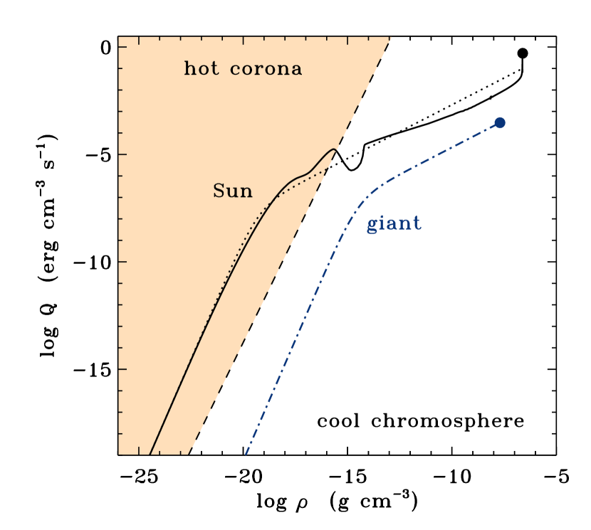
Figure 4.— Density dependence of the heating rate $Q$ defined in Equation (14) compared to the density dependence of the maximum radiative cooling rate from Equation (20) (dashed curve). For the Sun, a numerical model (black solid curve) compares favorably with a simple analytic “bridging” between the near-star ($Q\propto\rho^{1/2}$) and distant ($Q\propto\rho^{9/4}$) scalings discussed in the text (black dotted curve). For an example evolved giant star (blue dot-dashed curve), the transition to the steeper density dependence occurs to the right of the cooling boundary.

Figure 4 compares the modeled heating rates with the “maximum cooling boundary” implied by Equation (20). The solar model crosses the boundary, and thus undergoes a transition to a hot corona. The solid curve was taken from a numerical model of fast solar wind from a polar coronal hole (Cranmer et al., 2007). On the other hand, a model for a representative late-type giant sits to the right of the cooling boundary, which implies that radiative losses can maintain the circumstellar temperature at chromospheric values of $\sim 10^{4}$ K even at large distances. The two models differ because the density at which $M_{\rm A}\approx 1$ (where the $Q$ curves undergo a change in slope) for the giant is several orders of magnitude larger than the corresponding density for the solar case. This density is an output of a given mass loss model and cannot be specified a priori.

In this section we develop a model for cool-star mass loss under the assumption of strong radiative cooling. In this case the Parker (1958) gas pressure driving mechanism cannot drive a significant outflow. However, when the flux of Alfvén waves is large, they can impart a strong bulk acceleration to the plasma due to wave pressure, which is a nondissipative net ponderomotive force exerted by virtue of wave propagation through an inhomogeneous medium (Bretherton & Garrett, 1968; Jacques, 1977). The subsequent calculation of $\dot{M}$ for a “cold wave-driven” stellar wind largely follows the development of Holzer et al. (1983) (see also Cranmer, 2009).

Three key assumptions are: (1) that the Alfvén wave amplitudes in the wind are larger than the local sound speeds, (2) that there is negligible wave damping between the stellar surface and the wave-modified critical point of the flow, and (3) that the critical point occurs far enough from the stellar surface that $f\approx 1$ there (i.e., the flux tube expansion becomes radial). A fourth assumption from Holzer et al. (1983)—which was initially not applied here but later found to be valid—is that the stellar wind is sub-Alfvénic at the critical point (i.e., that $M_{\rm A}\ll 1$ at the critical point). Cranmer (2009) constructed a set of numerical models for the cold polar outflows of T Tauri stars that did not make the fourth assumption, and found that for a wide range of parameters the assumption was justified. Thus, here we use the value of the critical radius given by Equation (35) of Holzer et al. (1983), in which all four of the above assumptions were applied, and

$$\frac{r_{\rm crit}}{R_{\ast}}\,\approx\,\frac{7/4}{1+(v_{\perp\ast}/V_{\rm esc})^{2}}\,\,.$$ (31)

Once the critical point radius is known, it becomes possible to use the known properties of the Alfvén waves to determine the wind velocity and density at the critical point. Holzer et al. (1983) found analytic solutions for these quantities in the limiting case of $M_{\rm A}\ll 1$ at the critical point. Here we describe a slightly more self-consistent way of computing $M_{\rm A}$ and the mass loss rate, but we also continue to use Equation (31) that was derived in the limit of $M_{\rm A}\ll 1$. There are three unknown quantities and three equations to constrain them. The three unknowns are the critical point values of the wind speed $u$, density $\rho$, and wave amplitude $v_{\perp}$. The first equation is the constraint that the right-hand side of the time-steady momentum equation must sum to zero at the critical point of the flow (e.g., Parker, 1958). For the conditions described above, this gives

$$\frac{2u_{\rm crit}^{2}}{r_{\rm crit}}-\frac{GM_{\ast}}{r_{\rm crit}^{2}}\,=\,0\,\,,$$ (32)

and it is solved straightforwardly for $u_{\rm crit}$. The second and third equations are, respectively, the definition of the critical point velocity in the “cold” limit of zero gas pressure,

$$u_{\rm crit}^{2}\,=\,\frac{v_{\perp}^{2}}{4}\left(\frac{1+3M_{\rm A}}{1+M_{\rm A}}\right)$$ (33)

and the conservation of wave action as given by Equation (13). The fact that $V_{\rm A}$ appears in these equations and depends on the (still unknown) density makes it difficult to find an explicit analytic solution for $\rho_{\rm crit}$. We again use iteration from an initial guess to reach a self-consistent solution for $u$, $\rho$, and $v_{\perp}$ at the critical point. The stellar wind’s mass loss rate is thus determined from $\dot{M}=4\pi r_{\rm crit}^{2}u_{\rm crit}\rho_{\rm crit}$.

Because the mass loss rate is set at the critical point, we do not need to specify the terminal speed $u_{\infty}$. For most implementations of the above model, the denominator in Equation (31) is close to unity and thus we have $u_{\rm crit}^{2}\approx V_{\rm esc}^{2}/7$, or that $u_{\rm crit}$ is about 38% of the presumed value of $u_{\infty}$. Of course, there have been stellar wind models with nonmonotonic radial variations of $u(r)$, with $u_{\rm crit}>u_{\infty}$ (e.g., Falceta-Gonçalves et al., 2006). It is also possible for “too much” mass to be driven past the critical point, such that parcels of gas may be decelerated to stagnation at some height above $r_{\rm crit}$ and thus would want to fall back down towards the star. In reality, this parcel would collide with other parcels that are still accelerating, and a stochastic collection of shocked clumps is likely to result. Interactions between these parcels may result in an extra degree of collisional heating that could act as an extended source of gas pressure to help maintain a mean net outward flow. Situations similar to this have been suggested to occur in the outflows of pulsating cool stars (Bowen, 1988; Struck et al., 2004), T Tauri stars (Cranmer, 2008), and luminous blue variables (van Marle et al., 2009).

3.3. Combining Hot and Cold Models

A proper treatment of a stellar wind powered by MHD turbulence—and accelerated by a combination of gas pressure and wave pressure effects—requires a self-consistent numerical solution to the conservation equations (e.g., Cranmer et al., 2007; Suzuki, 2007; Cohen et al., 2009; Airapetian et al., 2010). However, in this paper, we explore simpler ways of estimating the combined effects of both processes.

Sections 3.1 and 3.2 gave us independent estimates for the mass loss rate assuming only gas pressure or wave pressure were active in the flux tube of interest. We refer to these two mass loss rates as $\dot{M}_{\rm hot}$ and $\dot{M}_{\rm cold}$, respectively. It seems clear that when one of these values is much larger than the other, then one process is dominant and the actual mass loss rate should be close to that larger value. For the manifestly “hot” example of the Sun, we found that $\dot{M}_{\rm hot}/\dot{M}_{\rm cold}\approx 20$, which correctly implies that gas pressure driving is dominant. For most examples of late-type giants with $L_{\ast}>10\,L_{\odot}$, the ratio $\dot{M}_{\rm hot}/\dot{M}_{\rm cold}$ was found to decrease to values between about 0.1 and 3. This could mean that gas and wave pressure gradients are of the same order of magnitude for these stars.

One of the most straightforward things that can be done is to assume the combined effect of gas and wave pressure produces a mass loss rate equal to the sum of the two individual components, $\dot{M}_{\rm hot}+\dot{M}_{\rm cold}$. This preserves the idea that one dominant mechanism should determine $\dot{M}$ when the other would predict a negligibly small effect. It also makes sense based on Equation (24), which shows how the energy fluxes sum together linearly in the internal energy equation. If there were multiple sources of input energy flux, Equation (26) would show that the resulting mass loss rate should be proportional to their sum.

However, there is one complication that hinders us from simply adding together $\dot{M}_{\rm hot}$ and $\dot{M}_{\rm cold}$. The calculation of $\dot{M}_{\rm hot}$ from Section 3.1 contains the assumption that the TR turbulent heating always obeys the near-star density scaling $Q\propto\rho^{1/2}$. It therefore predicts that all stars eventually undergo a transition to a hot corona. For some stars (like the late-type giant in Figure 4), however, we know that there should be no corona and it is erroneous to assume that $\dot{M}_{\rm hot}$ has any real meaning. Thus, for each model we compute the wind speed at the TR from mass flux conservation,

$$u_{\rm TR}\,=\,\frac{\dot{M}_{\rm hot}}{4\pi R_{\ast}^{2}f_{\rm TR}\rho_{\rm TR}}\,\,,$$ (34)

and we demand that for $\dot{M}_{\rm hot}$ to have a consistent interpretation, the TR Mach number $M_{\rm A,TR}=u_{\rm TR}/V_{\rm A,TR}$ should be much smaller than one. As expected, this condition was found to be violated for late-type giants having $L_{\ast}\gtrsim 100\,L_{\odot}$. Thus, in these cases we should replace $\dot{M}_{\rm hot}$ with either a drastically reduced value or zero—the latter in cases where the $Q(\rho)$ curve always falls to the right of the maximum cooling boundary in Figure 4. After some experimentation, we found that reducing the initially computed value of $Q_{\rm TR}$ by a factor of $\exp(-4M_{\rm A,TR}^{2})$ does a reasonably good job of reproducing the result of using a more consistent $Q(\rho)$ function. Thus, we propose that the summing of the “hot” and “cold” mass loss rates be done with the following approximate expression,

$$\dot{M}\,\approx\,\dot{M}_{\rm cold}+\dot{M}_{\rm hot}\exp\left(-4M_{\rm A,TR}^{2}\right)$$ (35)

where $\dot{M}_{\rm hot}$ and $M_{\rm A,TR}$ are computed using the assumptions of Section 3.1 and $\dot{M}_{\rm cold}$ is computed using the model given in Section 3.2.

4. Magnetic Activity and Rotation

An important ingredient in the above models—which remains unspecified for most stars—is the photospheric filling factor $f_{\ast}$. It is now well-known that both $f_{\ast}$ and the magnetic flux density $B_{\ast}f_{\ast}$ exhibit significant correlations with stellar rotation speed (Saar & Linsky, 1986; Marcy & Basri, 1989; Montesinos & Jordan, 1993; Saar, 2001). For many stars the rotation rate also scales with age, chromospheric activity, and coronal X-ray emission (Skumanich, 1972; Noyes et al., 1984; Pizzolato et al., 2003; Mamajek & Hillenbrand, 2008). A prevalent explanation for these correlations is that an MHD dynamo amplifies the magnetic flux in proportion to the large-scale energy input from differential rotation (e.g., Parker, 1979; Montesinos et al., 2001; Bushby, 2003; Moss & Sokoloff, 2009; Christensen et al., 2009; Işık et al., 2011).

In this section we construct an empirical scaling relation that will allow a reasonably accurate determination of $f_{\ast}$ as a function of $P_{\rm rot}$ and the other stellar parameters. Other estimates of this relationship have been made in the past (Montesinos & Jordan, 1993; Stȩpien, 1994; Saar, 1996a, 2001; Cuntz et al., 1998; Fawzy et al., 2002). However, since our goal is to apply this relation to stellar wind acceleration (in open flux tubes that cover a subset of the inferred $f_{\ast}$ area) and to evolved giants (which are greatly undersampled in observational studies of $f_{\ast}$), we aim to reanalyze the existing data rather than rely on other published scalings.

Table 1 lists the properties of 29 stars that have reliable measurements of their fundamental parameters, rotation rates, and either independent or combined values of $B_{\ast}$ and $f_{\ast}$. The sources for these values are given as numbered references in the final column. In many cases the available sources gave only a subset of the basic stellar parameters. When necessary, we used Equation (1) and information from the NASA/IPAC/NExScI Star and Exoplanet Database (NStED) to fill in missing values (see Berriman et al., 2010). Table 1 also gives approximate “quality factors” $q$ that describe the relative accuracy of the measurements, and in the Appendix we describe these factors in more detail.

It has been known for some time that, for dwarf stars, $B_{\ast}$ never appears to be very far from the equipartition field strength $B_{\rm eq}$ (e.g., Saar & Linsky, 1986). Figure 5 plots the ratio $B_{\ast}/B_{\rm eq}$ for the measurements in Table 1 that have separate determinations of $B_{\ast}$ and $f_{\ast}$. The sizes of the symbols are proportional to the observational quality factors, and all statistical fits and moments discussed below were weighted linearly with $q$. Figure 5(a) shows that there is no strong correlation of $B_{\ast}/B_{\rm eq}$ with $T_{\rm eff}$. Saar (1996a) found a slight increase in $B_{\ast}/B_{\rm eq}$ for the most rapid rotators ($P_{\rm rot}<3$ days), and Figure 5(b) shows that when more data are included this trend survives but is not strong. The power-law fit is consistent with a relationship $B_{\ast}\propto P_{\rm rot}^{-0.13}$, but we do not consider it significant enough to apply it below or to extrapolate it to longer rotation periods.

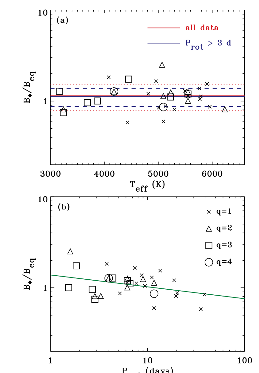
Figure 5.— Observational data for $B_{\ast}/B_{\rm eq}$ as a function of (a) effective temperature and (b) rotation rate. Solid lines in (a) show mean values for all data (red) and for only stars having $P_{\rm rot}>3$ days (blue). Dotted and dashed lines show regions within $\pm 1\sigma$ of the means. Quality factors are denoted by crosses ($q=1$), triangles ($q=2$), squares ($q=3$) and circles ($q=4$).

We found that the $q$-weighted mean value of $B_{\ast}/B_{\rm eq}$ for the entire sample (1.16, with standard deviation $\pm 0.38$) is only marginally higher than the mean value for the subset of slower rotating, non-saturated stars with $P_{\rm rot}>3$ days (1.13, with standard deviation $\pm 0.25$). Equation (6) gives the latter mean value, which we use in Section 5 for modeling the winds of the (generally slowly rotating) stars with observed mass loss rates. We also use Equation (6) to estimate $f_{\ast}$ for the cases where only the product $B_{\ast}f_{\ast}$ has been measured.

A primary indicator of stellar magnetic activity appears to be the photospheric filling factor $f_{\ast}$. There have been a number of different proposed ways to express the general anticorrelation between activity and rotation period. Noyes et al. (1984) found that indices of chromospheric activity correlate better with the so-called Rossby number $\mbox{Ro}\equiv P_{\rm rot}/\tau_{c}$, where $\tau_{c}$ is a measure of the convective turnover time, than with $P_{\rm rot}$ alone. For other data sets, however, the usefulness of the Rossby number has been called into question (Basri, 1986; Stȩpien, 1994). Saar (1991) postulated that $B_{\ast}f_{\ast}$ (and presumably also $f_{\ast}$ itself) is proportional to $\mbox{Ro}^{-1}$ (see also Montesinos & Jordan, 1993; Cuntz et al., 1998; Saar, 2001; Fawzy et al., 2002).

To compute the Rossby number for a given star, we need to know the convective turnover time $\tau_{c}$. Figure 6 compares several past calculations of $\tau_{c}$ with one another. For most stars we will utilize a parameterized fit to the set of ZAMS stellar models given by Gunn et al. (1998),

$$\tau_{c}=314.24\exp\left[-\left(\frac{T_{\rm eff}}{1952.5\,\mbox{K}}\right)-\left(\frac{T_{\rm eff}}{6250\,\mbox{K}}\right)^{18}\right]+0.002\,,$$ (36)

where $\tau_{c}$ is expressed in units of days and the fit is valid for the approximate range $3300\lesssim T_{\rm eff}\lesssim 7000$ K. Such a fit ignores how $\tau_{c}$ may depend on other stellar parameters besides effective temperature, but more recent sets of models (Landin et al., 2010; Barnes & Kim, 2010; Kitchatinov & Olemskoy, 2011) also found reasonably monotonic behavior as a function of $T_{\rm eff}$ for a broad range of stellar ages and masses.

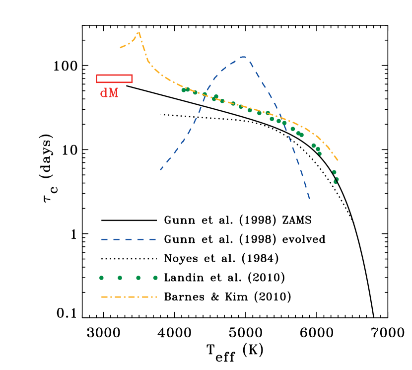
Figure 6.— Estimates of the convective turnover time $\tau_{c}$ as a function of $T_{\rm eff}$. ZAMS models of Gunn et al. (1998) were fit by Equation (36) (black solid curve). The Gunn et al. (1998) evolutionary track for a $2.2M_{\odot}$ star (blue dashed curve) outlines an upper limit for $\tau_{c}$ at intermediate temperatures. Local values of $\tau_{c}$ from Landin et al. (2010) (green symbols) and Barnes & Kim (2010) (orange dot-dashed curve), the parameterization given by Noyes et al. (1984) (black dotted curve), and the M dwarf estimate of $\tau_{c}\approx 70$ d used by Reiners et al. (2009) (red box labeled by “dM”) are also shown.

There are indications that the simple relationship between $\tau_{c}$ and $T_{\rm eff}$ seen for main-sequence stars is not universal. For example,

1. Low-mass M dwarfs (with $M_{\ast}\lesssim 0.35\,M_{\odot}$) are likely to be fully convective, and thus their dynamos are likely to be driven by fundamentally different processes than exist in more massive stars (Mullan & MacDonald, 2001; Reiners & Basri, 2007; Irwin et al., 2011). There is also some disagreement about the relevant $\tau_{c}$ values for these stars. Figure 6 shows that the models of Barnes & Kim (2010) exhibit a slight discontinuity at the fully convective boundary. The Reiners et al. (2009) semi-empirical estimate of $\tau_{c}\approx 70$ days for M dwarfs is about a factor of 2–3 lower than that of Barnes & Kim (2010). However, because the Reiners et al. (2009) value is in reasonable agreement with an extrapolation of Equation (36) to lower effective temperatures, we will just use this expression and not make any special adjustments to the Rossby numbers of fully convective M dwarfs.

2. Luminous evolved giants exhibit qualitatively different interior properties than do main sequence stars of similar $T_{\rm eff}$. Despite not having firm measurements of the magnetic activities of evolved giants, we will want to estimate $f_{\ast}$ for such stars in order to compute their mass loss rates. Gondoin (2005, 2007) found that the correlation between X-ray activity and rotation in G and K giants is consistent with that of main-sequence stars if the larger values of $\tau_{c}$ from the evolved models of Gunn et al. (1998) were used instead of the ZAMS values (see the blue dashed curve in Figure 6). Similarly, Hall (1994) calculated luminosity-dependent scaling factors that can be used to multiply the ZAMS value of $\tau_{c}$ to obtain a consistent relation between rotation and photometric activity (see also Choi et al., 1995). We found that the above results can be generally reproduced by multiplying the ZAMS value of $\tau_{c}$ by a factor $(g_{\odot}/g)^{0.23}$, which applies only for low-gravity subgiants and giants (i.e., only for $g<g_{\odot}$). In Section 5 we explore the extent to which this kind of approximate correction factor helps to explain the activity and mass loss of evolved stars.

A slightly different way of estimating the magnetic flux of a rotating star is to take advantage of a proposed “magnetic Bode’s law;” i.e., the conjecture that the star’s magnetic moment scales linearly with its angular momentum (Arge et al., 1995; Baliunas et al., 1996). Using the stellar parameters defined above, this corresponds approximately to

$$B_{\ast}f_{\ast}R_{\ast}^{3}\,\propto\,\frac{M_{\ast}R_{\ast}^{2}}{P_{\rm rot}}\,\,\,.$$ (37)

The above relationship does not take into account variations of the moment of inertia (for different stars) away from an idealized scaling of $I\sim M_{\ast}R_{\ast}^{2}$, and it assumes the magnetic moment is dominated by a large-scale dipole component. It is possible to test this idea with the data given in Table 1 by evaluating the correlation between $f_{\ast}$ and $M_{\ast}(R_{\ast}P_{\rm rot}B_{\ast})^{-1}$.

Figure 7 shows how the empirical set of $f_{\ast}$ values correlates with rotation period, Rossby number, and the proposed magnetic Bode’s law. Rather than use the Rossby number itself, we instead plot the data in Figure 7(b) as a function of a normalized ratio $\mbox{Ro}/\mbox{Ro}_{\odot}$, where according to Equation (36), the Sun’s Rossby number $\mbox{Ro}_{\odot}=1.96$. Such a normalization allows us to neglect any scaling discrepancies between “local” and “global” definitions of $\tau_{c}$ (e.g., Pizzolato et al., 2001; Landin et al., 2010). The Sun’s large range of measured $f_{\ast}$ values ($10^{-3}$ to $10^{-2}$) is indicated with a vertical bar, and it is likely that all other stars exhibit such a range on both rotational and dynamo-cycle time scales.

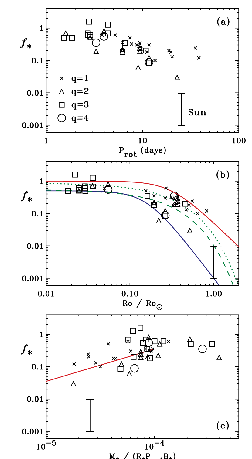
Figure 7.— Comparison of possible correlations between measured $f_{\ast}$ filling factors with (a) rotation rate, (b) Rossby number, and (c) a magnetic Bode’s law parameter (see Equation (37)). Solid curves in (b) denote the lower (blue) and upper (red) envelopes surrounding the data, and green curves show fitting formulae from Equations 2.3 (dotted; empirical) and 7.3 (dashed; theoretical) of Montesinos & Jordan (1993). Quality factors are denoted by the same symbols used in Figure 5, and the Sun’s range of $f_{\ast}$ is shown with a vertical bar.

Figures 7(a) and 7(c) show that the correlations with $P_{\rm rot}$ and the proposed magnetic Bode’s law are not especially strong. However, if all of the lowest quality ($q=1$) measurements were removed, the correlation with $P_{\rm rot}$ would be improved significantly. Figure 7(b) shows that the Rossby number seems to be a slightly better ordering parameter, and it compares the individual data points with several functional relationships. The blue and red solid curves are subjective fits to the minimum and maximum bounds on the envelope of data points, with

$$f_{\rm min}\,=\,\frac{0.5}{[1+(x/0.16)^{2.6}]^{1.3}}\,\,,$$ (38)

$$f_{\rm max}\,=\,\frac{1}{1+(x/0.31)^{2.5}}$$ (39)

where $x=\mbox{Ro}/\mbox{Ro}_{\odot}$. We also show empirical and theoretical fitting formulae from Montesinos & Jordan (1993). Other comparisons could also be made with relationships given by Cuntz et al. (1998), Fawzy et al. (2002), and others, but they all appear to fall near the green and red curves.

Note that for slow rotation rates (i.e., large Rossby numbers) the scaling laws shown in Figure 7(b) imply a significantly steeper decline of $f_{\ast}$ than has been suggested in the past. For example, Saar (1991) estimated $f_{\ast}\propto\mbox{Ro}^{-1}$, and Saar (1996a) estimated $f_{\ast}\propto P_{\rm rot}^{-1.8}$. On the other hand, our empirical upper and lower bounds suggest $f_{\rm max}\propto\mbox{Ro}^{-2.5}$ and $f_{\rm min}\propto\mbox{Ro}^{-3.4}$ respectively. This is similar to the observed relationship between Rossby number and X-ray activity. Mamajek & Hillenbrand (2008) found that the ratio of X-ray to bolometric luminosity $L_{\rm X}/L_{\rm bol}$ drops by about a factor of 700 as the Rossby number increases by a factor of ten from 0.25 to 2.5 (see also Wright et al., 2011). This corresponds very roughly to a power-law decrease of $\mbox{Ro}^{-2.85}$. Its agreement with the behavior of $f_{\ast}$ shown above is also consistent with existing empirical correlations between X-rays and magnetic activity (Pevtsov et al., 2003).

In addition to the rotational scaling of $f_{\ast}$ with Ro, there is also likely to be a “basal” lower limit on the outer atmospheric activity of a star (e.g., Schrijver, 1987; Cuntz et al., 1999; Bercik et al., 2005; Takeda & Takada-Hidai, 2011; Pérez Martínez et al., 2011). Whether this lower limit is the result of acoustic waves, a turbulent dynamo, or some other physical process, there is probably a minimum value of $f_{\ast}$ that is independent of rotation rate. For example, Bercik et al. (2005) found that turbulent dynamos in main sequence stars can generate a flux density $B_{\ast}f_{\ast}\approx 4$ G without much variation from spectral types F0 to M0. Using Equation (6) for $B_{\ast}$, we can estimate a basal filling factor for these stars of $f_{\ast}\approx 0.001$–0.002, which is close to the Sun’s minimum value. However, since it is still uncertain whether or not the Sun has exhibited truly basal flux conditions in recent years (Cliver & Ling, 2011), we will set a slightly lower value of $f_{\rm basal}=10^{-4}$ to be used in the mass loss models below.

Before moving on to apply the empirical values of $f_{\ast}$ to our model of mass loss, we emphasize that the measurements do not directly provide the filling factor of open magnetic flux tubes. Ideally, Zeeman broadening measurements should be sensitive to the total flux in strong magnetic elements on the stellar surface, no matter whether the field lines are closed or open. In many cases, however, the closed-loop active regions have significantly stronger local field strengths than the open regions. Therefore the closed-field regions are likely to dominate the spectral line broadening that gives rise to the observational determinations of $f_{\ast}$ (see the Appendix). Without spatially resolved magnetic field measurements, we do not yet have a definitive way to predict how a given star divides up its flux tubes between open and closed. Mestel & Spruit (1987) claimed that as the rotation rate increases (from slow values similar to the Sun’s), the relative fraction of closed field regions should first increase, then eventually it should decrease as centrifugal forces strip the field lines open. We can speculate that the spread in the measured $f_{\ast}$ data may tell us something about the closed and open fractions. Because closed-loop active regions tend to have stronger fields than open coronal holes, the lower and upper envelopes that surround the data in Figure 7(b) could be good proxies for the filling factors of open and closed regions, respectively. More specifically, we hypothesize that $f_{\rm min}$ is seen when no active regions are present on the visible surface (i.e., $f_{\rm min}\approx f_{\rm open}$) and that $f_{\rm max}$ is seen when active regions dominate the observed magnetic flux. This idea is tested, in a limited way, in Section 5.2.

5. Results

Here we present the results of solving the mass loss equations derived in Section 3 using the empirical estimates for the rotational dependence of the magnetic filling factor derived in Section 4. For hot coronal mass loss, we assumed values for the dimensionless parameters $\alpha_{0}=0.5$, $h=0.5$, and $\theta=1/3$. As discussed above, these values were “calibrated” from our more detailed knowledge of the Sun’s coronal heating and wind acceleration. Our use of these values for other stars is an extrapolation that can be tested by comparison with observed mass loss rates.

5.1. Database of Stellar Mass Loss Rates

Figure 8 is a broad overview of observed stellar mass loss. It plots the locations of individual stars in a Hertzsprung-Russell type diagram with their mass loss rates shown as symbol color (see also de Jager et al., 1988). A box illustrates the approximate regime of parameter space covered by the models developed in this paper; it extends from the main sequence up through the regime of the so-called “hybrid chromosphere” stars (Hartmann et al., 1980), and possibly also into the parameter space of cool luminous supergiants. In addition to the cool-star data discussed below, we also include in Figure 8 measured mass loss rates of hot, massive stars (Waters et al., 1987; Lamers et al., 1999; Mokiem et al., 2007; Searle et al., 2008), FGK supergiants (de Jager et al., 1988), AGB stars (Bergeat & Chevallier, 2005; Guandalini, 2010), red giants in globular clusters (Mészáros et al., 2009), and M dwarfs in pre-cataclysmic variable binaries (Debes, 2006). Many of these stars are not included in the subsequent analysis because we have no firm rotation periods or magnetic activity indices for them.

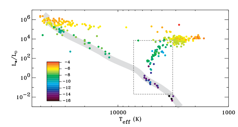
Figure 8.— Hertzsprung-Russell diagram showing observed mass loss rates. The color scale at lower-left specifies log $\dot{M}$, where $\dot{M}$ is measured in $M_{\odot}$ yr^-1. An estimate for the ZAMS is shown in gray, and the approximate domain of parameter space covered by the models of this paper is outlined by a black dotted box.

Table 2 lists the properties of 47 stars for which our knowledge appears to be complete enough to be able to compare theoretical and observed values of $\dot{M}$. For the Sun, the range of volume-integrated mass loss rates comes from Wang (1998). The sources for all listed values are given as numbered references that continue the sequence started in Table 1; the citations corresponding to numbers 1–32 are given in Table 1. In cases where $T_{\rm eff}$, $\log\,g$, or [Fe/H] were estimated from the PASTEL database (Soubiran et al., 2010), we averaged together multiple measurements when more than one was given. In the few cases where the same star appears in both Table 1 and Table 2, for consistency’s sake we will recompute $f_{\ast}$ from the star’s rotation period when calculating theoretical mass loss rates (see Section 5.2).

For binary systems with astrospheric measurements of $\dot{M}$ (see, e.g., Wood et al., 2002), the numbers given are assumed to be the sum of both stars’ mass loss rates. We list that same value for both components and denote it with “(A$+$B).” We did not utilize the published astrospheric measurements of Proxima Cen and 40 Eri A, which gave only upper limits on $\dot{M}$, and $\lambda$ And and DK UMa, which had uncertain detections of astrospheric H I Ly$\alpha$ absorption (Wood et al., 2005a, b).

At the bottom of Table 2 we list three stars that have parameters at the outer bounds of what we intend to model. They are test cases for the limits of applicability of the physical processes summarized in Section 3. EV Lac is an active M dwarf and flare star that probably has a fully convective interior (e.g., Osten et al., 2010). Such stars may exhibit qualitatively different mechanisms of mass loss and rotation-activity correlation than do stars higher up the main sequence (Mullan, 1996; Reiners & Basri, 2007; Irwin et al., 2011; Martínez-Arnáiz et al., 2011; Vidotto et al., 2011). V Hya is an N-type carbon star with an extended and asymmetric AGB envelope and evidence for rapid rotation (Barnbaum et al., 1995; Knapp et al., 1999). 89 Her is a post-AGB yellow supergiant with multiple detections of circumstellar nebular material (Sargent & Osmer, 1969; Bujarrabal et al., 2007). It is worthwhile to investigate to what extent the mass loss mechanisms proposed in this paper could be applicable to these kinds of stars.

Not all stars in Table 2 have precise measurements for their rotation period. For 61 Vir and 70 Oph B, we used published estimates of the rotation period that were obtained from the known correlation between rotation and chromospheric Ca II activity (Baliunas et al., 1996). For essentially all stars more luminous than $\sim 5\,L_{\odot}$ (with the exception of HR 6902; see Griffin, 1988) we estimated $P_{\rm rot}$ via spectroscopic determinations of $v\sin i$ from the rotational broadening of photospheric absorption lines. The inclination angle $i$ is the main unknown quantity. Chandrasekhar & Münch (1950) found that for an isotropically distributed set of inclination vectors, the mean value of $\sin i$ is $\pi/4$. Thus, we estimate a mean rotation period

$$\langle P_{\rm rot}\rangle\,=\,\frac{2\pi R_{\ast}}{(4/\pi)\,v\sin i}\,\,.$$ (40)

Note that the median of $\sin i$ for an isotropic distribution is not equal to the mean; the former is given by $\sqrt{3}/2$. In order to encompass both values, as well as the majority of “most likely” values of $P_{\rm rot}$, we can adopt generous uncertainty limits for which we will estimate $f_{\ast}$ and the other derived quantities for mass loss. For the isotropic distribution of direction vectors, the quantity $\sin i$ falls between 0.5 and 1 approximately 87% of the time. This is a reasonably good definition for uncertainty bounds that would correspond to $\pm 1.5\sigma$ if the distribution were Gaussian. Thus, for stars with only $v\sin i$ measurements, we use the following values as error bars on the derived rotation period:

$$\frac{2}{\pi}\lesssim\frac{P_{\rm rot}}{\langle P_{\rm rot}\rangle}\lesssim\frac{4}{\pi}\,\,.$$ (41)

5.2. Comparing Predictions with Observations

We applied the combined model for mass loss that culminated in Equation (35) to the stars listed in Table 2. Below we show results of direct forward modeling; i.e., utilizing a known relationship for $f_{\ast}$ as a function of Rossby number. First, however, we wanted to investigate whether or not a single monotonic relationship for $f_{\ast}(\mbox{Ro})$ could produce mass loss rates that were even remotely close to the measured values. Thus, we produced trial grids of models in which $f_{\ast}$ was treated as a free parameter. For each star, we varied $f_{\ast}$ from $10^{-5}$ to 1 and found the empirical value of the filling factor ($f_{\rm emp}$) for which the modeled value of $\dot{M}$ matched the observed value given in Table 2. For the four binaries that have only systemic measurements of $\dot{M}$ we summed the model predictions for each component and made a single comparison with the observations.

Figure 9 shows the result of this process of “working backwards” from the measured mass loss rates. The empirically constrained $f_{\rm emp}$ values are plotted against Rossby number, which is defined with (a) the simple Gunn et al. (1998) ZAMS value for $\tau_{c}$ (Equation (36)) and (b) a gravity-modified version of $\tau_{c}$ that gives giants larger convective overturn times. We varied the exponent in the gravity modification term and found that multiplying the ZAMS $\tau_{c}$ by $(g_{\odot}/g)^{0.18}$ gives the narrowest distribution of $f_{\ast}$ versus Ro. The optimal exponent of 0.18 is very close to the value of 0.23 that we found reproduced the results of Hall (1994) and Gondoin (2005, 2007). In Figure 9 we also show the same curves from Figure 7(b) that outline the measured range of filling factors. The lower envelope curve $f_{\rm min}$, defined in Equation (38), appears to be a good match to the gravity-modified empirical values $f_{\rm emp}$. This provides circumstantial evidence that $f_{\rm min}$ is indeed an appropriate proxy for the filling factor of open flux tubes as a function of Rossby number.

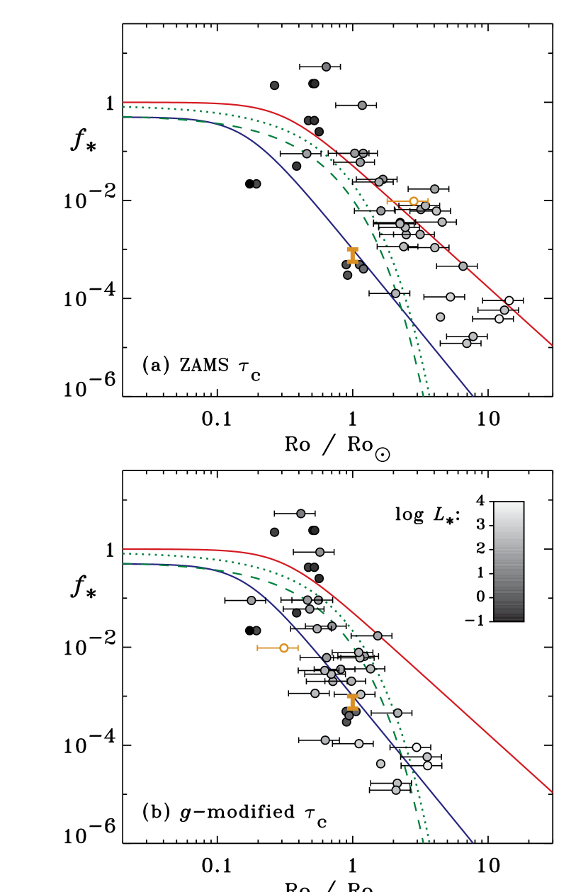
Figure 9.— Empirical $f_{\rm emp}$ filling factors computed to match measured mass loss rates. Rossby numbers were computed in two ways: (a) directly from Equation (36), and (b) multiplying $\tau_{c}$ from Equation (36) by $(g_{\odot}/g)^{0.18}$. Symbol shading is proportional to $\log(L_{\ast}/L_{\odot})$, and the curves are the same as those in Figure 7(b). The thick orange bar denotes the Sun’s empirical range of values (computed from the small variation in $\dot{M}$). The open orange circle denotes V Hya, the only one of the three test cases (at bottom of Table 2) that gave a realistic solution for $f_{\rm emp}$.

We now put aside the empirical estimates for the filling factor and use only Equation (38) for $f_{\ast}=f_{\rm min}$ in the remainder of this paper. Table 3 shows some of the predicted properties of stellar coronae and winds for the 47 stars in our database. There were only seven stars for which Equation (38) gave a filling factor below the adopted “floor” value of $f_{\rm basal}=10^{-4}$; we replaced $f_{\rm min}$ with $f_{\rm basal}$ in those cases. Table 3 also gives $F_{\rm H,TR}$, the coronal heat flux deposited at the TR for each star. It may be useful to use this to predict the X-ray flux associated with open-field regions on these stars, but we should note that the closed-field regions (which we do not model) are likely to dominate the observed X-ray emission. We also list the various components of Equation (35) so that the contributions of gas pressure and wave pressure can be assessed (see below).

Table 3Theoretical Wind Properties of Cool Stars

Name	Ro	$\log f_{\rm min}$	$B_{\ast}$ (G)	$\log F_{H,TR}$	$\dot{M}_{\rm hot}/\dot{M}_{\rm cold}$	$\log M_{\rm A,TR}$	$-\log(\dot{M}/[M_{\odot}\mbox{yr}^{-1}])$
Sun	1.960	-2.996	1513.05	6.14	19.73	-2.42	13.44
$\alpha$ Cen A (G2 V)	2.074	-3.078	1308.79	6.17	11.43	-2.17	13.21
$\alpha$ Cen B (K0 V)	1.755	-2.835	1545.97	5.62	51.73	-2.93	14.09
70 Oph A (K0 V)	0.996	-2.025	1666.45	5.99	194.1	-3.25	13.43
70 Oph B (K5 V)	1.027	-2.067	2130.57	4.55	417.3	-4.50	15.17
$\epsilon$ Eri (K4.5 V)	0.519	-1.174	1832.80	5.97	977.4	-3.94	13.31
61 Cyg A (K5 V)	1.107	-2.173	2145.92	4.59	246.1	-4.43	15.15
$\epsilon$ Ind (K5 V)	0.755	-1.646	1941.88	5.15	551.7	-4.22	14.25
36 Oph A (K5 V)	0.923	-1.918	1927.79	5.67	228.1	-3.63	13.84
36 Oph B (K5 V)	1.021	-2.059	1973.54	5.51	173.1	-3.66	14.16
$\xi$ Boo A (G8 V)	0.381	-0.853	1788.75	6.69	1335	-3.59	12.42
$\xi$ Boo B (K4 V)	0.340	-0.755	2620.92	4.83	5964	-5.37	14.68
61 Vir (G5 V)	1.765	-2.843	1524.08	5.99	27.96	-2.63	13.56
$\delta$ Eri (K0 IV)	1.844	-2.907	1077.96	5.77	12.04	-2.18	12.72
$\alpha$ Boo (K1.5 III)	4.217	-4.000	411.54	5.23	0.57	-0.31	10.33
$\alpha$ Tau (K5 III)	4.183	-4.000	270.35	5.17	0.75	0.11	9.88
$\gamma$ Dra (K5 III)	4.097	-4.000	301.38	5.24	0.85	-0.12	9.99
HR 6902 (G9 IIb)	3.157	-3.692	287.82	6.11	1.28	0.13	9.86
$\beta$ And (M0 III)	1.229	-2.321	311.31	5.61	0.47	-0.85	8.86
$\beta$ UMi (K4 III)	6.960	-4.000	262.45	5.32	0.85	0.28	9.72
$\mu$ UMa (M0 III)	2.182	-3.152	165.83	5.81	0.63	0.68	7.93
$\alpha$ TrA (K2 II-III)	7.010	-4.000	270.87	5.55	1.25	-0.13	9.32
$\lambda$ Vel (K4 Ib-II)	5.808	-4.000	136.66	5.67	2.15	1.05	8.47
BD $+$01 3070 (RGB)	1.122	-2.192	792.36	6.49	2.36	-1.48	10.14
BD $+$05 3098 (RGB)	1.600	-2.700	553.26	6.37	0.50	-0.63	9.08
BD $+$09 2574 (RGB)	3.001	-3.618	632.02	5.74	0.49	-0.62	10.17
BD $+$09 2870 (RGB)	2.249	-3.196	476.21	6.00	0.37	-0.17	8.68
BD $+$10 2495 (RGB)	2.390	-3.284	602.67	6.01	0.51	-0.62	9.83
BD $+$12 2547 (AGB)	2.657	-3.439	378.07	5.98	0.60	0.10	9.20
BD $+$17 3248 (RHB)	1.259	-2.355	493.93	6.81	0.65	-0.53	9.05
BD $+$18 2757 (AGB)	1.400	-2.508	384.43	6.55	0.32	-0.03	8.05
BD $+$18 2976 (RGB)	2.218	-3.175	464.10	5.96	0.32	-0.12	8.54
BD $-$03 5215 (RHB)	1.095	-2.157	583.84	7.06	1.91	-0.90	9.36
HD 083212 (RGB)	1.361	-2.467	464.86	6.20	0.23	-0.44	8.07
HD 101063 (SGB)	0.813	-1.744	1312.86	6.26	40.43	-2.65	11.31
HD 107752 (AGB)	2.171	-3.145	524.60	6.08	0.42	-0.37	9.05
HD 110885 (RHB)	0.909	-1.897	575.05	7.06	2.02	-0.97	9.17
HD 111721 (RGB)	1.379	-2.486	609.98	6.42	0.61	-0.91	9.64
HD 115444 (RGB)	1.919	-2.965	491.45	6.14	0.34	-0.31	8.82
HD 119516 (RHB)	0.945	-1.950	483.08	7.24	1.29	-0.62	8.80
HD 121135 (AGB)	1.071	-2.126	502.44	6.68	0.60	-0.68	8.47
HD 122956 (RGB)	1.218	-2.309	444.03	6.27	0.19	-0.38	7.88
HD 135148 (RGB)	1.033	-2.075	394.38	5.99	0.07	-0.25	6.98
HD 195636 (RHB)	0.350	-0.779	435.75	7.64	3.38	-0.88	7.90
EV Lac (M3.5 V)	0.0706	-0.313	3005.25	2.72	2641	-8.15	17.78
V Hya (N6, AGB)	0.609	-1.367	12.39	6.53	1.32	1.99	4.34
89 Her (F2 Ib)	27.12	-4.000	43.59	1.92	0.05	-1.11	11.15

Figure 10 compares the theoretical and measured mass loss rates with one another as a function of $L_{\ast}$. For the four binary systems listed in Table 2 with combined A$+$B mass loss rates, we separated the measured value into two pieces using the modeled $\dot{M}$ ratio for the two components. (This was done for this figure only because the measured rates are shown as a function of a single star’s luminosity.) For stars with only $v\sin i$ rotation period estimates, we used Equation (40) to compute $\dot{M}$ for the central plotting symbol and the entries in Table 3, and we recomputed $\dot{M}$ for the lower and upper limits given by Equation (41) to obtain the error bars. Figure 10(b) shows a comparison with the semi-empirical scaling law proposed by Schröder & Cuntz (2005), with

$$\dot{M}_{\rm SC}\,=\,\eta\frac{L_{\ast}R_{\ast}}{M_{\ast}}\left(\frac{T_{\rm eff}}{4000\,\mbox{K}}\right)^{3.5}\left(1+\frac{g_{\odot}}{4300\,g}\right)$$ (42)

where $L_{\ast}$, $R_{\ast}$, and $M_{\ast}$ are assumed to be in solar units. For this plot we computed the normalization constant $\eta$ such that the average modeled mass loss rate would equal the average measured mass loss rate for all 47 stars. Averages were taken using the logarithm of $\dot{M}$ so that all stars would contribute to the average comparably. We found $\eta=8.5\times 10^{-14}$ $M_{\odot}$ yr^-1, which is within the error bars of the Schröder & Cuntz (2005) value.

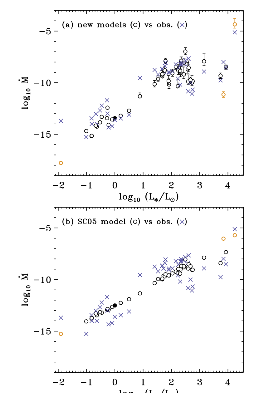
Figure 10.— Comparison of modeled (open circles) and measured (blue crosses) mass loss rates for the stars in Table 2, plotted as $\log\dot{M}$ versus stellar luminosity. Panels show (a) the standard model developed in this paper, and (b) the empirical scaling relation of Schröder & Cuntz (2005). The Sun is shown as a filled black circle, and the three test-case stars from the bottom of Table 2 are shown in orange. Vertical error bars in (a) correspond to models computed for the $P_{\rm rot}$ range of Equation (41).

Overall, our “standard model” (i.e., Equation (35) with $\alpha_{0}=0.5$, $h=0.5$, and $\theta=1/3$) appears to match the measured mass loss rates reasonably well. We emphasize that this model does not contain any arbitrary $\eta$ normalization factors. For the three test-case stars at the bottom of Table 2, however, our model does not do as well. The model underpredicts the mass loss from the dM flare star EV Lac by at least four orders of magnitude, and it also fails for the F supergiant 89 Her by a slightly smaller amount. For EV Lac and other flare-active M dwarfs, it is possible that coronal mass ejections and other episodic sources of energy (Mullan, 1996) could be responsible for the bulk of the observed mass loss. For the carbon star V Hya, the reasonably good agreement between the model and measurements is probably a coincidence, since our model does not include the dusty radiative transfer or strong radial pulsations that are likely to be important for AGB stars.

It is interesting to highlight the case of the moderately rotating K dwarfs $\epsilon$ Eri, 70 Oph, and 36 Oph, which Holzwarth & Jardine (2007) found to have anomalously high mass loss rates. They concluded that the observed magnetic fluxes for these stars were insufficient to produce their dense outflows. For these stars, our modeled mass loss rates tended to be about a factor of 10–20 below the measured values. However, these models were computed using $f_{\rm min}$ from Equation (38). The measured values of $f_{\ast}$ given in Table 1 for these stars are larger than their corresponding $f_{\rm min}$ values by factors ranging from 3 to 20. If instead these values were used, our modeled mass loss rates would be in better agreement with the astrospheric observations of Wood et al. (2005a).

We also developed a statistical measure of how well a given model agrees with the measured database of mass loss rates. We defined a straightforward least-squares parameter

$$\chi^{2}\,=\,\frac{1}{N}\sum_{i=1}^{N}\left[\log\dot{M}_{i}(\mbox{model})-\log\dot{M}_{i}(\mbox{obs})\right]^{2}$$ (43)

where the total number of comparisons ($N=40$) excludes the final three test cases in Table 2 and counts each of the four A$+$B binaries as one. When $\chi^{2}<1$, then (on average) the modeled and measured mass loss rates are within an order of magnitude of one another. Table 4 summarizes the results, including comparisons with other published empirical prescriptions. The $\eta$ normalization factors for each of these scaling laws were computed similarly as the factor in Equation (42) above. Note that our standard model appears to be a significant improvement over both the popular Reimers (1975, 1977) and Schröder & Cuntz (2005) scalings.

Table 4Mass Loss “Goodness of Fit”

Model	$\chi^{2}$
This paper (standard model)	0.650
This paper (ZAMS $\tau_{c}$)	1.575
This paper ($h=0.25$)	0.794
This paper ($h=1$)	0.564
This paper ($h=3$)	0.504
This paper ($\theta=0.2$)	0.620
This paper ($\theta=0.5$)	0.707
This paper (all [Fe/H] $=0$)	0.647
This paper ($\dot{M}=\dot{M}_{\rm hot}+\dot{M}_{\rm cold}$)	0.703
This paper ($\alpha$ from Trampedach & Stein 2011)	0.770
Reimers (1975, 1977)	1.260
Mullan (1978), Equation (4a)	3.768
Nieuwenhuijzen & de Jager (1990)	2.356
Catelan (2000), Equation (A1)	1.924
Schröder & Cuntz (2005)	1.131

To further explore the proposed model, we varied some of the modeling parameters described in Section 3. Varying the TR filling factor exponent $\theta$ did not have much of an effect on $\chi^{2}$. However, varying the flux height scaling factor $h$ did change $\chi^{2}$ significantly. We found that a larger value of $h\approx 3$ gives much better agreement with the measured mass loss rates than does the standard value of $h=0.5$ (see Table 4). We decided not to adopt this larger value, though, because it falls well outside the range of empirically determined $h$ values for the Sun’s corona.

We also tried removing some of the imposed complexity of the standard model to see if simpler assumptions would give adequate results. Removing the gravity-dependent modification factor of $(g_{\odot}/g)^{0.18}$ from the definition of the convective overturn time resulted in significantly poorer agreement with the data (i.e., more than double the $\chi^{2}$ of the standard model). We explored the importance of metallicity by replacing the published [Fe/H] by purely solar values ([Fe/H] $=0$). This actually improved the value of $\chi^{2}$ from the standard model, but only by $<1$%. Removing the exponential factor in Equation (35) gave a slightly higher value of $\chi^{2}$ (8% larger than the standard model).

We also noted that the theoretical photospheric Alfvén wave fluxes from Musielak & Ulmschneider (2002a) exhibited a strong dependence on the convective mixing length parameter (i.e., $F_{\rm A\ast}\propto\alpha^{2.1}$). Thus, instead of simply assuming $\alpha=2$ as in the standard model, we created a linear regression fit to the tabulated simulation results of Trampedach & Stein (2011), who found empirical values of $\alpha$ between 1.6 and 2.2 depending on $T_{\rm eff}$, $\log\,g$, and $M_{\ast}$. We used the following approximate fit

$$\alpha_{\rm TS}\,\approx\,1.91-\frac{T_{\rm eff}}{6181\,\mbox{K}}+\frac{\log\,g}{5.58}+\frac{M_{\ast}}{19.1\,M_{\odot}}$$ (44)

and did not allow $\alpha_{\rm TS}$ to be less than 1.6 or greater than 2.2. Thus, we multiplied the value of $F_{\rm A\ast}$ from Equation (7) by a factor of $(\alpha_{\rm TS}/2)^{2.1}$. The predicted mass loss rates for the Table 2 stars had about an 18% higher value of $\chi^{2}$ than the standard model, so we did not pursue this mixing length prescription any further.

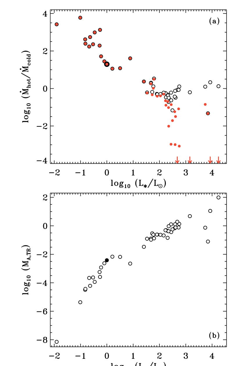
Figure 11.— Illustrations of the relative importance of “hot” versus “cold” mass loss mechanisms. (a) Ratio of hot to cold modeled values for $\dot{M}$ (open circles) compared with the modified ratio $\dot{M}_{\rm hot}\exp(-4M_{\rm A,TR}^{2})/\dot{M}_{\rm cold}$ (red filled circles). (b) Mach number at the TR, $M_{\rm A,TR}=u_{\rm TR}/V_{\rm A,TR}$. The Sun is shown as a thicker black circle in (a) and a filled black circle in (b).

For additional context about the hot and cold mass loss models described in Section 3.3, Figure 11 shows the ratio $\dot{M}_{\rm hot}/\dot{M}_{\rm cold}$ for the 47 modeled stars as well as the TR Mach number $M_{\rm A,TR}=u_{\rm TR}/V_{\rm A,TR}$. It is clear that the dwarf stars are dominated by hot coronae, and the stellar wind outflow is still negligibly small at the coronal base. However, as the luminosity exceeds $\sim 50\,L_{\odot}$ for the giant stars, the hot coronal contribution goes away and the acceleration becomes dominated by wave pressure.

Figure 12 examines how the plasma number density at the transition region, $n_{\rm TR}=\rho_{\rm TR}/m_{\rm H}$, depends on stellar rotation. Holzwarth & Jardine (2007) assumed $n_{\rm TR}\propto\Omega^{0.6}\propto P_{\rm rot}^{-0.6}$ (see also Ivanova & Taam, 2003). Although our models do not follow a single universal relation for both giants and dwarfs, the proposed scaling (or one slightly steeper) may be appropriate for certain sub-populations of stars. For the dwarf stars with well-determined rotation periods, it is interesting that the Sun’s computed value of $n_{\rm TR}$ is larger than that of stars having higher magnetic activity. Equation (22) shows that the dependence on filling factor is weak (i.e., about $f_{\ast}^{0.19}$ for $\theta=1/3$), so the variation comes mostly from the other stellar parameters. This seems to stand in contrast with other observational determinations of coronal electron densities, where $n$ tends to increase with activity (Güdel, 2004). However, X-ray determinations of number density are probably dominated by closed-field active regions, which are not necessarily correlated with the regions driving the stellar wind.

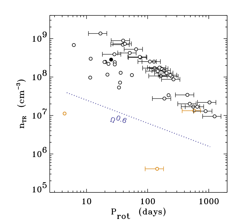
Figure 12.— Plasma number density at the TR plotted as a function of stellar rotation period. Symbols are the same as in Figure 10.

5.3. Predictions for Idealized Stellar Parameters

In addition to the above comparisons with the individual stars of Table 2, we also created some purely theoretical sets of stellar models and computed $\dot{M}$ for them. We began with the ZAMS model parameters given by Girardi et al. (2000), and we assumed solar metallicity for a range of constant rotation rates. This gave rise to a two-dimensional grid of models (varying $T_{\rm eff}$ and $P_{\rm rot}$) for main sequence stars. Because the modeled stars are all high-gravity dwarfs, we used only Equation (36) for $\tau_{c}$, in combination with Equation (38) for $f_{\rm min}$ as a function of Rossby number.

Figure 13 shows the resulting mass loss rates as a function of $T_{\rm eff}$ and $P_{\rm rot}$. If we had not utilized a basal “floor” on $f_{\ast}$, we would have predicted a steep drop-off in mass loss for $T_{\rm eff}\gtrsim 7000$ K, at which the Gunn et al. (1998) expression for $\tau_{c}$ decreases rapidly. However, because of the floor, there appear to be reasonably strong mass loss rates up to the point at which subsurface convection zones disappear at $T_{\rm eff}\gtrsim 9000$ K. There is a slightly discontinuous dip in the predicted basal mass flux around $T_{\rm eff}\approx 6100$ K that arises because of the iteration for ${\cal R}$, $\rho_{\rm TR}$, and $Q_{\rm TR}$. If the calculation of these quantities is halted after only one iteration, the final value of $\dot{M}$ varies more smoothly as a function of $T_{\rm eff}$. We plan to utilize a more self-consistent non-WKB model of Alfvén wave reflection in future versions of this work.

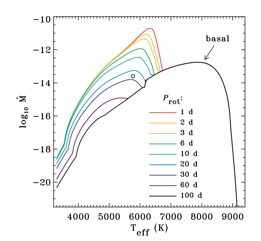
Figure 13.— Theoretical predictions of $\dot{M}$ for main sequence stars, plotted as a function of $T_{\rm eff}$. Differently colored curves show a range of assumed rotation periods (see labels for values). The Sun is indicated by an open circle.

The mass loss rates shown in Figure 13 are almost all due to the hot coronal processes discussed in Section 3.1. Thus, it is possible to simplify the components of Equation (26) in order to obtain an approximate scaling relation for $\dot{M}$ that is reasonable for these main sequence stellar models. Ignoring the weakest dependences on some stellar parameters (i.e., factors with exponents less than or equal to $1/7$), we found

$$\frac{\dot{M}}{10^{-10}\,M_{\odot}/\mbox{yr}}\,\sim\,\left(\frac{R_{\ast}}{R_{\odot}}\right)^{16/7}\left(\frac{L_{\ast}}{L_{\odot}}\right)^{-2/7}$$

$$\times\,\left(\frac{F_{\rm A\ast}}{10^{9}\,\mbox{erg}\,\,\mbox{cm}^{-2}\,\,\mbox{s}^{-1}}\right)^{12/7}f_{\ast}^{(4+3\theta)/7}\,\,,$$ (45)

which reproduces the curves in Figure 13 to within about an order of magnitude. Despite the fact that this scaling formula is relatively easy to apply, we do not recommend its use in stellar evolution or population synthesis calculations. Once stars leave the main sequence, Equation (45) is no longer a good approximation.

We also computed a time-dependent mass loss rate for the evolutionary track of a star having $M_{\ast}=1\,M_{\odot}$. There is evidence that the wind from the “young Sun” was significantly denser than it is today, and this more energetic outflow may have been important to early planetary evolution (e.g., Wood, 2006; Güdel, 2007; Sterenborg et al., 2011; Suzuki, 2011). We used the BaSTI evolutionary track plotted in Figure 1 (Pietrinferni et al., 2004) for the time variation of $R_{\ast}$ and $L_{\ast}$. We grafted on a model of rotational evolution for a solar-mass star from Figure 6(a) of Denissenkov et al. (2010). For late ages ($t\gtrsim 100$ Myr, or $\log t\gtrsim 8$), this model has approximately $P_{\rm rot}\propto t^{0.54}$. Such an age scaling is well within the range of empirically determined power laws ($t^{0.5}$ to $t^{0.6}$) obtained from young solar analogs (e.g., Barnes, 2003; Güdel, 2007).

Figure 14(a) shows how the luminosity and two dimensionless parameters related to the rotational dynamo (Ro and $f_{\rm min}$) vary as a function of age for this model. Note that prior to about $t\approx 70$ Myr the Rossby number is small enough that the filling factor appears to be saturated near its maximum assumed value of 0.5. At very late times, when the star begins to ascend the red giant branch, the Rossby number decreases again because of the increase in $\tau_{c}$ with decreasing $T_{\rm eff}$ and gravity. We utilized the $(g_{\odot}/g)^{0.18}$ correction factor when computing $\tau_{c}$, but it was relatively unimportant until the star left the main sequence.

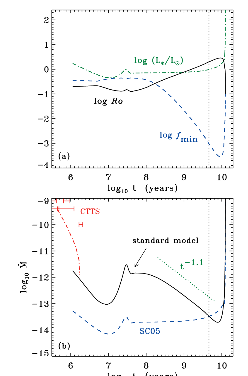
Figure 14.— Theoretical predictions of stellar wind properties for an evolving solar-mass star. (a) Base-10 logarithms of luminosity (green dot-dashed curve), Rossby number (black solid curve), and $f_{\rm min}$ (blue dashed curve) plotted as a function of age in years. (b) Our standard model for $\dot{M}$ (black solid curve), compared with the Schröder & Cuntz (2005) scaling (blue dashed curve) and an ideal power-law $t^{-1.1}$ decline with increasing age (green dotted curve). A model and observations of CTTS are shown for comparison (red error bars and dot-dashed curve).

Figure 14(b) gives our prediction for the age variation of the a solar-type star’s mass loss rate. For ages between about $t\approx 0.2$ and 7 Gyr the decrease in mass loss appears to be fit approximately by a power law, with $\dot{M}\propto t^{-1.1}$. This is a significantly shallower age dependence than the $t^{-2}$ decline suggested by Wood et al. (2002) on the basis of astrosphere measurements. We note that if the rotation period was the only variable to change with time, Equation (45) would give something like $\dot{M}\propto P_{\rm rot}^{-2.4}$ (for $f_{\ast}=f_{\rm min}$ and $\theta=1/3$). Thus, a more rapid increase of $P_{\rm rot}$ with age—such as the $t^{0.85}$ dependence in the solar-mass rotational model of Landin et al. (2010)—would give rise to a steeper age-$\dot{M}$ relationship more similar to that of Wood et al. (2002).

For comparison, Figure 14(b) also shows that the Schröder & Cuntz (2005) scaling law predicts a much smaller range of mass loss variation for the young Sun than does the present model. We also show a model (Cranmer, 2008, 2009) and measurements (Hartigan et al., 1995) for classical T Tauri stars (CTTS) at the youngest ages. It is clear that for $t\lesssim 10$ Myr some additional physical processes must be included (e.g., accretion-driven turbulence on the stellar surface) to successfully predict mass loss rates.

6. Discussion and Conclusions

The primary aim of this paper was to develop a new generation of physically motivated models of the winds of cool main sequence stars and evolved giants. These models follow the production of MHD turbulent motions from subsurface convection zones to their eventual dissipation and escape through the stellar wind. The magnetic activity of these stars is taken into account by extending standard age-activity-rotation indicators to include the evolution of the filling factor of strong magnetic fields in stellar photospheres. The winds of G and K dwarf stars tend to be driven by gas pressure from hot coronae, whereas the cooler outflows of red giants are supported mainly by Alfvén wave pressure. We tested our model of combined “hot” and “cold” winds by comparing with the observed mass loss rates of 47 stars, and we found that this model produces better agreement with the data than do published scaling laws. We also made predictions for the parametric dependence of $\dot{M}$ on $T_{\rm eff}$ and rotation period for main sequence stars, and on age for a one solar mass evolutionary track.

The eventual goal of this project is to provide a straightforward algorithm for predicting the mass loss rates of cool stars for use in calculations of stellar evolution and population synthesis. A brief stand-alone subroutine called BOREAS has been developed to implement the model described in this paper. This code is written in the Interactive Data Language (IDL) and it is included with this paper as online-only material. This code is also provided, with updates as needed, on the first author’s web page. Packaged with the code itself are data files that allow the user to reproduce many of the results shown in Section 5.

In order to further test the conjecture that Alfvén waves and turbulence drive cool-star winds, the models need to be expanded from the simple scaling laws of Section 3 to fully self-consistent solutions of the mass, momentum, and energy conservation equations along open flux tubes. Modeling the full radial dependence of density, temperature, magnetic field strength, and outflow speed would eliminate our reliance on approximate factors like $h$ and $\theta$. We believe that the models of Cranmer et al. (2007) for the solar wind, and Cranmer (2008) for T Tauri stars, can be extended straightforwardly and applied to other types of stars. However, there are many other approaches to producing self-consistent and/or three-dimensional models that should be explored (e.g., Airapetian et al., 2000, 2010; Holzwarth & Jardine, 2005; Schrijver & Title, 2005; Falceta-Gonçalves et al., 2006; Suzuki, 2007; Vidotto et al., 2009; Cohen et al., 2009; Cohen, 2011).

There are additional ways that our simplified models of coronal energy balance (Section 3.1) and wave-pressure driving (Section 3.2) may be improved:

1. Our standard assumption for the outflow speed in a coronal wind was $u_{\infty}=V_{\rm esc}$. However, Judge (1992) found that many stars have significantly smaller terminal speeds. It should be possible to use something like the Schwadron & McComas (2003) solar wind scaling law to estimate the peak temperature in the corona, and thus apply the Parker (1958) theory of gas pressure acceleration to compute the wind speed.

2. We assumed in Section 3.1 that $r_{\rm TR}\approx R_{\ast}$. However, Schröder & Cuntz (2005) estimated that some low-gravity stars should exhibit “puffed up” chromospheres with a fractional extent given by the final term in parentheses in Equation (42). We applied this correction factor to the modeled values of $r_{\rm TR}$ and $\dot{M}_{\rm hot}$ for the stars in Table 2. Doing so yielded significant differences from the standard model only for stars having $\dot{M}_{\rm cold}\gg\dot{M}_{\rm hot}$, i.e., the combined model value of $\dot{M}$ was relatively unchanged in those cases. However, in general there may be other stars for which this kind of correction factor needs to be considered in more detail.

3. We also assumed that the flux height scaling factor $h$ took on a single constant value for all stars. It may be useful to explore extending the Schröder & Cuntz (2005) idea of gravity-dependent spatial expansion to this parameter as well. The $\chi^{2}$ results shown in Table 4 suggest that a larger value of $h\approx 3$ could be appropriate for many of the low-gravity stars in our observational database, whereas the range $h\approx 0.5$–1 is probably best for main sequence stars like the Sun.

4. The flux of energy $F_{\rm A\ast}$ in kink/Alfvén waves in the photosphere may depend on other parameters that we have not considered. Musielak & Ulmschneider (2002a) found that the flux is rather sensitive to $B_{\ast}/B_{\rm eq}$ in the photosphere, so departures from our assumed value of 1.13 may give rise to significantly different predictions. Also, Musielak & Ulmschneider (2002b) examined the sensitivity to metallicity and found that lower $Z/Z_{\odot}$ tends to give lower values of $F_{\rm A\ast}$ for $T_{\rm eff}\lesssim 6000$ K. Preliminary tests showed that this effect does not strongly affect the mass loss rates derived in this paper. However, a varying metallicity should also change other properties of the convection—including the effective mixing length $\alpha$ parameter—thus possibly making this effect more important.

5. Instead of assuming a simple monotonic dependence of the open-field filling factor on Rossby number, it may be possible to construct realistic surface distributions of active regions for a given activity level and rotation period, and model the opening up of flux tubes by both stellar winds and centrifugal forces (Mullan & Steinolfson, 1983; Mestel & Spruit, 1987; Jardine, 2004; Holzwarth & Jardine, 2005; Cohen et al., 2009).

To continue testing and refining these models, it is also important to utilize the newest and most accurate measurements of stellar mass loss rates (see, e.g., Schröder & Cuntz, 2007; Willson, 2009; Catelan, 2009; Mauron & Josselin, 2011; Vieytes et al., 2011) and magnetic fields (Donati & Landstreet, 2009; Vlemmings et al., 2011).

Finally, we emphasize that a complete description of late-type stellar winds requires the incorporation of other physical processes besides Alfvén waves and turbulence. The outer atmospheres of cool stars are also likely to be powered by acoustic or longitudinal MHD waves (Cuntz, 1990; Buchholz et al., 1998), episodic flares or coronal mass ejections (Mullan, 1996; Aarnio et al., 2009), and large-amplitude pulsations (Bowen, 1988; de Jager et al., 1997; Willson, 2000). It is well known that radiative driving should not be neglected for AGB stars and red supergiants, and it may be important for Cepheids (Neilson & Lester, 2008) and horizontal branch stars (Vink & Cassisi, 2002) as well.

Appendix A Notes on Stellar Magnetic Field Measurements

In this work we focus on observations of unpolarized spectral lines sensitive to Zeeman splitting by stellar magnetic fields (e.g., Robinson, 1980). The resulting “Zeeman broadened” line profiles are valuable probes of both the intensity-weighted mean absolute value of the field strength (i.e., $B_{\ast}=\langle I_{\rm B}|B|\rangle/\langle I_{\rm B}\rangle$, where $I_{\rm B}$ is the continuum intensity in the magnetic regions) and the intensity-weighted fraction of the visible stellar hemisphere that is covered by these fields (i.e., the filling factor $f_{\ast}$). These detections are thus weighted towards the brightest regions of the stellar surface; i.e., plage or network regions. However, this technique allows detection of more topologically complex fields, and thus more comprehensive values of $f_{\ast}$ and $B_{\ast}$, than does the use of circular polarization. The latter exhibits significant signal cancellation when there are multiple oppositely directed patches of magnetic field in the same resolution element. In many cases, however, only the disk-averaged magnetic flux density ($B_{\ast}f_{\ast}$) can be determined reliably from Zeeman broadened spectra and not the separate values of $B_{\ast}$ and $f_{\ast}$ (see also Rüedi et al., 1997; Anderson et al., 2010).

Many details of the observations of the stars discussed in Section 4 were given by Saar & Linsky (1985, 1986) and Saar (1990, 1991, 1996a, 1996b, 2001). The approximate quality factors listed in Table 1 span the range from low ($q=1$) to high ($q=4$) relative confidence in the derived magnetic parameters. The values for $q$ were assigned based on a combination of the following properties of the spectroscopic data and its magnetic analysis:

1. Detections using lines with longer wavelengths and higher Landé $g_{\rm eff}$ factors are given higher $q$ values. The ratio of the strength of the Zeeman effect to the nonmagnetic Doppler width is $\Delta\lambda_{\rm B}/\Delta\lambda_{\rm D}$, where $\Delta\lambda_{\rm B}\propto g_{\rm eff}\lambda^{2}$ is the Zeeman splitting amplitude and $\Delta\lambda_{\rm D}\propto\lambda$ is the nonmagnetic Doppler width. Thus, the relative detectability of the effect increases as $g_{\rm eff}\lambda$.

2. Spectra with higher signal-to-noise (S/N) ratios and higher spectral resolution (${\cal R}=\lambda/\Delta\lambda$) tend to have higher quality (see, e.g., Saar, 1988), although a longer wavelength measurement can trump better ${\cal R}$. For example, the greater magnetic sensitivity at large $\lambda$ can lead to partial resolution of the individual Zeeman components (Saar & Linsky, 1985).

3. The simultaneous analysis of larger numbers of lines (especially with higher $g_{\rm eff}$) contributes to a good quality measurement (Rüedi et al., 1997). It is additionally helpful for the lines to be free of blends and for any rotational broadening to be small (i.e., $v\sin i\lesssim 10$ km s^-1); see also Saar (1988).

4. Finally, the method and quality of line modeling—including the level of detail in the magnetic radiative transfer, the atmospheric models used, details of integration over the stellar disk, and the treatment of line blends—vary widely. This field has seen a continual improvement in the sophistication of these models, with an attendant increase in our understanding of the measurement and systematic uncertainties (e.g., Anderson et al., 2010; Shulyak et al., 2010).

We chose to exclude several published observations from the list of stars given in Table 1. We did not use the M dwarf data presented by Reiners et al. (2009) because these stars all tended to sit in the saturated region of Figure 7 (i.e., $\mbox{Ro}/\mbox{Ro}_{\odot}<0.1$), and thus do not contribute to improving our knowledge of the rotation dependence of $f_{\ast}$. We did not include the measured field of the F6 main sequence star HD 68456 (Anderson et al., 2010) because we do not attempt to model the outflows of stars significantly hotter than the Sun. Also, its combined strong field and high Rossby number point to a possible transition to a different type of magnetic activity from that described by the standard cool-star age-activity-rotation relationship (see also Böhm-Vitense et al., 2002).

References

- Aarnio et al. (2009) Aarnio, A. N., Stassun, K. G., & Matt, S. P. 2009, in AIP Conf. Proc. 1094, 15th Cambridge Workshop on Cool Stars, Stellar Systems, and the Sun, ed. E. Stempels (Melville, NY: AIP), 337
- Airapetian et al. (2010) Airapetian, V. S., Carpenter, K. G., & Ofman, L. 2010, ApJ, 723, 1210
- Airapetian et al. (2000) Airapetian, V. S., Ofman, L., Robinson, R. D., Carpenter, K., & Davila, J. 2000, ApJ, 528, 965
- Alonso et al. (1996) Alonso, A., Arribas, S., & Martínez-Roger, C. 1996, A&AS, 117, 227
- Anderson et al. (2010) Anderson, R. I., Reiners, A., & Solanki, S. K. 2010, A&A, 522, A81
- Arge et al. (1995) Arge, C. N., Mullan, D. J., & Dolginov, A. Z. 1995, ApJ, 443, 795
- Ayres et al. (2007) Ayres, T. R., Brown, A., & Harper, G. M. 2007, ApJ, 658, L107
- Baliunas et al. (1996) Baliunas, S., Sokoloff, D., & Soon, W. 1996, ApJ, 457, L99
- Barnbaum et al. (1995) Barnbaum, C., Morris, M., & Kahane, C. 1995, ApJ, 450, 862
- Barnes (2003) Barnes, S. A. 2003, ApJ, 586, 464
- Barnes & Kim (2010) Barnes, S. A., & Kim, Y.-C. 2010, ApJ, 721, 675
- Basri (1986) Basri, G. 1986, in 4th Cambridge Workshop on Cool Stars, Stellar Systems, and the Sun, ed. M. Zeilik & D. Gibson (Berlin: Springer), 184
- Baumann et al. (2010) Baumann, P., Ramírez, I., Meléndez, J., Asplund, M., & Lind, K. 2010, A&A, 519, A87
- Bercik et al. (2005) Bercik, D. J., Fisher, G. H., Johns-Krull, C. M., & Abbett, W. P. 2005, ApJ, 631, 529
- Bergeat & Chevallier (2005) Bergeat, J., & Chevallier, L. 2005, A&A, 429, 235
- Berger & Title (2001) Berger, T. E., & Title, A. M. 2001, ApJ, 553, 449
- Berriman et al. (2010) Berriman, G. B., et al. 2010, in ASP Conf. Ser. 434, Astronomical Data Analysis Software and Systems XIX, ed. Y. Mizumoto, K.-I. Morita, & M. Ohishi (San Francisco: ASP), 119
- Bingert & Peter (2011) Bingert, S., & Peter, H. 2011, A&A, 530, A112
- Boehringer & Hensler (1989) Boehringer, H., & Hensler, G. 1989, A&A, 215, 147
- Böhm-Vitense et al. (2002) Böhm-Vitense, E., Robinson, R., Carpenter, K., & Mena-Werth, J. 2002, ApJ, 569, 941
- Bonfils et al. (2005) Bonfils, X., Delfosse, X., Udry, S., Santos, N. C., Forveille, T., & Ségransan, D. 2005, A&A, 442, 635
- Bowen (1988) Bowen, G. H. 1988, ApJ, 329, 299
- Breech et al. (2009) Breech, B., Matthaeus, W. H., Cranmer, S. R., Kasper, J., & Oughton, S. 2009, J. Geophys. Res., 114, A09103
- Bretherton & Garrett (1968) Bretherton, F. P., & Garrett, C. J. R. 1968, Proc. Roy. Soc. London A, 302, 529
- Buchholz et al. (1998) Buchholz, B., Ulmschneider, P., & Cuntz, M. 1998, ApJ, 494, 700
- Bujarrabal et al. (2007) Bujarrabal, V., van Winckel, H., Neri, R., Alcolea, J., Castro-Carrizo, A., & Deroo, P. 2007, A&A, 468, L45
- Bushby (2003) Bushby, P. J. 2003, MNRAS, 342, L15
- Carney et al. (2008) Carney, B. W., Gray, D. F., Yong, D., Latham, D. W., Manset, N., Zelman, R., & Laird, J. B. 2008, AJ, 135, 892
- Carpenter et al. (1999) Carpenter, K. G., Robinson, R. D., Harper, G. M., Bennett, P. D., Brown, A., & Mullan, D. J. 1999, ApJ, 521, 382
- Castor et al. (1975) Castor, J. I., Abbott, D. C., & Klein, R. I. 1975, ApJ, 195, 157
- Catelan (2000) Catelan, M. 2000, ApJ, 531, 826
- Catelan (2009) Catelan, M. 2009, Ap&SS, 320, 261
- Cayrel de Strobel et al. (2001) Cayrel de Strobel, G., Soubiran, C., & Ralite, N. 2001, A&A, 373, 159
- Chandrasekhar & Münch (1950) Chandrasekhar, S., & Münch, G. 1950, ApJ, 111, 142
- Choi et al. (1995) Choi, H.-J., Soon, W., Donahue, R. A., Baliunas, S. L., & Henry, G. W. 1995, PASP, 107, 744
- Christensen et al. (2009) Christensen, U. R., Holzwarth, V., & Reiners, A. 2009, Nature, 457, 167
- Cliver & Ling (2011) Cliver, E. W., & Ling, A. G. 2011, Sol. Phys., in press
- Cohen (2011) Cohen, O. 2011, MNRAS, in press, arXiv:1107.2275
- Cohen et al. (2009) Cohen, O., Drake, J. J., Kashyap, V. L., & Gombosi, T. I. 2009, ApJ, 699, 1501
- Coleman (1968) Coleman, P. J., Jr. 1968, ApJ, 153, 371
- Cortés et al. (2009) Cortés, C., Silva, J. R. P., Recio-Blanco, A., Catelan, M., Do Nascimento, J. D., & De Medeiros, J. R. 2009, ApJ, 704, 750
- Cranmer (2008) Cranmer, S. R. 2008, ApJ, 689, 316
- Cranmer (2009) Cranmer, S. R. 2009, ApJ, 706, 824
- Cranmer (2010) Cranmer, S. R. 2010, ApJ, 710, 676
- Cranmer & van Ballegooijen (2005) Cranmer, S. R., & van Ballegooijen, A. A. 2005, ApJS, 156, 265
- Cranmer et al. (2007) Cranmer, S. R., van Ballegooijen, A. A., & Edgar, R. J. 2007, ApJS, 171, 520
- Cuntz (1990) Cuntz, M. 1990, ApJ, 353, 255
- Cuntz et al. (1999) Cuntz, M., Rammacher, W., Ulmschneider, P., Musielak, Z. E., & Saar, S. H. 1999, ApJ, 522, 1053
- Cuntz et al. (1998) Cuntz, M., Ulmschneider, P., & Musielak, Z. E. 1998, ApJ, 493, L117
- Danziger & Faber (1972) Danziger, I. J., & Faber, S. M. 1972, A&A, 18, 428
- Davis (1955) Davis, L., Jr. 1955, Phys. Rev., 100, 1440
- Debes (2006) Debes, J. H. 2006, ApJ, 652, 636
- DeCampli (1981) DeCampli, W. M. 1981, ApJ, 244, 124
- de Jager et al. (1997) de Jager, C., Lobel, A., & Israelian, G. 1997, A&A, 325, 714
- de Jager et al. (1988) de Jager, C., Nieuwenhuijzen, H., & van der Hucht, K. A. 1988, A&AS, 72, 259
- de Medeiros & Mayor (1999) de Medeiros, J. R., & Mayor, M. 1999, A&AS, 139, 433
- Denissenkov et al. (2010) Denissenkov, P. A., Pinsonneault, M., Terndrup, D. M., & Newsham, G. 2010, ApJ, 716, 1269
- DeWarf et al. (2010) DeWarf, L. E., Datin, K. M., & Guinan, E. F. 2010, ApJ, 722, 343
- Dmitruk et al. (2002) Dmitruk, P., Matthaeus, W. H., Milano, L. J., Oughton, S., Zank, G. P., & Mullan, D. J. 2002, ApJ, 575, 571
- Donati & Landstreet (2009) Donati, J.-F., & Landstreet, J. D. 2009, ARA&A, 47, 333
- Dupree (1986) Dupree, A. K. 1986, ARA&A, 24, 377
- Dupree et al. (2009) Dupree, A. K., Smith, G. H., & Strader, J. 2009, AJ, 138, 1485
- Eggen (1996) Eggen, O. J. 1996, AJ, 111, 466
- Eggenberger et al. (2008) Eggenberger, P., Miglio, A., Carrier, F., Fernandes, J., & Santos, N. C. 2008, A&A, 482, 631
- Falceta-Gonçalves et al. (2006) Falceta-Gonçalves, D., Vidotto, A. A., & Jatenco-Pereira, V. 2006, MNRAS, 368, 1145
- Favata et al. (2000) Favata, F., Micela, G., & Reale, F. 2000, A&A, 354, 1021
- Fawzy & Cuntz (2011) Fawzy, D. E., & Cuntz, M. 2011, A&A, 526, A91
- Fawzy et al. (2002) Fawzy, D. E., Stȩpień, K., Ulmschneider, P., Rammacher, W., & Musielak, Z. E. 2002, A&A, 386, 994
- Fernandes et al. (1998) Fernandes, J., Lebreton, Y., Baglin, A., & Morel, P. 1998, A&A, 338, 455
- Ferraro & Plumpton (1958) Ferraro, C. A., & Plumpton, C. 1958, ApJ, 127, 459
- Gai et al. (2008) Gai, N., Bi, S.-L., & Tang, Y.-K. 2008, Chinese J. Astron. Astrophys., 8, 591
- Girardi et al. (2000) Girardi, L., Bressan, A., Bertelli, G., & Chiosi, C. 2000, A&AS, 141, 371.
- Gnat & Sternberg (2007) Gnat, O., & Sternberg, A. 2007, ApJS, 168, 213
- Gondoin (2005) Gondoin, P. 2005, A&A, 444, 531
- Gondoin (2007) Gondoin, P. 2007, A&A, 464, 1101
- Grevesse & Sauval (1998) Grevesse, N., & Sauval, A. J. 1998, Space Sci. Rev., 85, 161
- Griffin (1988) Griffin, R. E. M. 1988, JRASC, 82, 49
- Guandalini (2010) Guandalini, R. 2010, A&A, 513, A4
- Güdel (2004) Güdel, M. 2004, A&A Rev., 12, 71
- Güdel (2007) Güdel, M. 2007, Living Rev. Solar Phys., 4, 3
- Gunn et al. (1998) Gunn, A. G., Mitrou, C. K., & Doyle, J. G. 1998, MNRAS, 296, 150
- Hall (1994) Hall, D. S. 1994, Mem. Soc. Astron. Italiana, 65, 73
- Hammer (1982) Hammer, R. 1982, ApJ, 259, 767
- Hammer et al. (1996) Hammer, R., Nesis, A., Moore, R. L., Suess, S. T., & Musielak, Z. M. 1996, in ASP Conf. Ser. 109, 9th Cambridge Workshop on Cool Stars, Stellar Systems, and the Sun, ed. R. Pallavicini & A. Dupree (San Francisco, ASP), 525
- Hansteen & Leer (1995) Hansteen, V. H., & Leer, E. 1995, J. Geophys. Res., 100, 21577
- Harper et al. (1995) Harper, G. M., Wood, B. E., Linsky, J. L., Bennett, P. D., Ayres, T. R., & Brown, A. 1995, ApJ, 452, 407
- Hartigan et al. (1995) Hartigan, P., Edwards, S., & Ghandour, L. 1995, ApJ, 452, 736
- Hartmann et al. (1980) Hartmann, L., Dupree, A. K., & Raymond, J. C. 1980, ApJ, 236, L143
- Hartmann & MacGregor (1980) Hartmann, L., & MacGregor, K. B. 1980, ApJ, 242, 260
- Hearn (1988) Hearn, A. G. 1988, in Mass Outflows from Stars and Galactic Nuclei, ed. L. Bianchi & R. Gilmozzi (Dordrecht: Kluwer), 79
- Heinemann & Olbert (1980) Heinemann, M., & Olbert, S. 1980, J. Geophys. Res., 85, 1311
- Hekker & Aerts (2010) Hekker, S., & Aerts, C. 2010, A&A, 515, A43
- Höfner (2011) Höfner, S. 2011, in ASP Conf. Ser., Why Galaxies Care About AGB Stars II, ed. F. Kerschbaum, T. Lebzelter, & R. Wing (San Francisco: ASP), in press, arXiv:1102.5268
- Hollweg (1978) Hollweg, J. V. 1978, Rev. Geophys. Space Phys., 16, 689
- Hollweg (1986) Hollweg, J. V. 1986, J. Geophys. Res., 91, 4111
- Holzer & Axford (1970) Holzer, T. E., & Axford, W. I. 1970, ARA&A, 8, 31
- Holzer et al. (1983) Holzer, T. E., Flå, T., & Leer, E. 1983, ApJ, 275, 808
- Holzwarth & Jardine (2005) Holzwarth, V., & Jardine, M. 2005, A&A, 444, 661
- Holzwarth & Jardine (2007) Holzwarth, V., & Jardine, M. 2007, A&A, 463, 11
- Hossain et al. (1995) Hossain, M., Gray, P. C., Pontius, D. H., Jr., Matthaeus, W. H., & Oughton, S. 1995, Phys. Fluids, 7, 2886
- Irwin et al. (2011) Irwin, J., Berta, Z. K., Burke, C. J., Charbonneau, D., Nutzman, P., West, A. A., & Falco, E. E. 2011, ApJ, 727, 56
- Işık et al. (2011) Işık, E., Schmitt, D., & Schüssler, M. 2011, A&A, 528, A135
- Ivanova & Taam (2003) Ivanova, N., & Taam, R. E. 2003, ApJ, 599, 516
- Jacques (1977) Jacques, S. A. 1977, ApJ, 215, 942
- Janson et al. (2009) Janson, M., et al. 2009, MNRAS, 399, 377
- Jardine (2004) Jardine, M. 2004, A&A, 414, L5
- Jenkins et al. (2009) Jenkins, J. S., Ramsey, L. W., Jones, H. R. A., Pavlenko, Y., Gallardo, J., Barnes, J. R., & Pinfield, D. J. 2009, ApJ, 704, 975
- Jokipii & Davis (1969) Jokipii, J. R., & Davis, L., Jr. 1969, ApJ, 156, 110
- Judge (1992) Judge, P. G. 1992, in ASP Conf. Ser. 26, 7th Cambridge Workshop on Cool Stars, Stellar Systems, and the Sun, ed. M. Giampapa & J. Bookbinder (San Francisco, ASP), 403
- Judge & Stencel (1991) Judge, P. G., & Stencel, R. E. 1991, ApJ, 371, 357
- Kervella et al. (2008) Kervella, P., et al. 2008, A&A, 488, 667
- Kiraga & Stȩpień (2007) Kiraga, M., & Stȩpień, K. 2007, Acta Astron., 57, 149
- Kirsch et al. (2001) Kirsch, T., Baade, R., & Reimers, D. 2001, A&A, 379, 925
- Kitchatinov & Olemskoy (2011) Kitchatinov, L. L., & Olemskoy, S. V. 2011, MNRAS, 411, 1059
- Knapp et al. (1999) Knapp, G. R., Dobrovolsky, S. I., Ivezić, Z., Young, K., Crosas, M., Mattei, J. A., & Rupen, M. P. 1999, A&A, 351, 97
- Kovári et al. (2004) Kovári, Z., Strassmeier, K. G., Granzer, T., Weber, M., Oláh, K., & Rice, J. B. 2004, A&A, 417, 1047
- Kovtyukh et al. (2004) Kovtyukh, V. V., Soubiran, C., & Belik, S. I. 2004, A&A, 427, 933
- Kudritzki (2010) Kudritzki, R.-P. 2010, Astron. Nachr., 331, 459
- Lafon & Berruyer (1991) Lafon, J.-P. J., & Berruyer, N. 1991, A&A Rev., 2, 249
- Lambert et al. (1986) Lambert, D. L., Gustafsson, B., Eriksson, K., & Hinkle, K. H. 1986, ApJS, 62, 373
- Lamers & Cassinelli (1999) Lamers, H. J. G. L. M., & Cassinelli, J. P. 1999, Introduction to Stellar Winds (Cambridge: Cambridge University Press)
- Lamers et al. (1999) Lamers, H. J. G. L. M., Haser, S., de Koter, A., & Leitherer, C. 1999, ApJ, 516, 872
- Landin et al. (2010) Landin, N. R., Mendes, L. T. S., & Vaz, L. P. R. 2010, A&A, 510, A46
- Leer et al. (1982) Leer, E., Holzer, T. E., & Flå, T. 1982, Space Sci. Rev., 33, 161
- Leitherer (2010) Leitherer, C. 2010, in ASP Conf. Ser. 425, Hot and Cool: Bridging Gaps in Massive Star Evolution, ed. C. Leitherer, P. Bennett, P. Morris, & J. van Loon (San Francisco, ASP), 171
- Lighthill (1952) Lighthill, M. J. 1952, Proc. Roy. Soc. London A, 211, 564
- Linsky & Haisch (1979) Linsky, J. L., & Haisch, B. M. 1979, ApJ, 229, L27
- Mamajek & Hillenbrand (2008) Mamajek, E. E., & Hillenbrand, L. A. 2008, ApJ, 687, 1264
- Marcy & Basri (1989) Marcy, G. W., & Basri, G. 1989, ApJ, 345, 480
- Marigo & Aringer (2009) Marigo, P., & Aringer, B. 2009, A&A, 508, 1539
- Marshall (1996) Marshall, K. P. 1996, MNRAS, 280, 977
- Martínez-Arnáiz et al. (2011) Martínez-Arnáiz, R. M., López-Santiago, J., Crespo-Chacón, I., & Montes, D. 2011, MNRAS, 414, 2629
- Masana et al. (2006) Masana, E., Jordi, C., & Ribas, I. 2006, A&A, 450, 735
- Massarotti et al. (2008) Massarotti, A., Latham, D. W., Stefanik, R. P., & Fogel, J. 2008, AJ, 135, 209
- Matthaeus et al. (1999) Matthaeus, W. H., Zank, G. P., Oughton, S., Mullan, D. J., & Dmitruk, P. 1999, ApJ, 523, L93
- Mauron & Josselin (2011) Mauron, N., & Josselin, E. 2011, A&A, 526, A156
- Mazzotta et al. (1998) Mazzotta, P., Mazzitelli, G., Colafrancesco, S., & Vittorio, N. 1998, A&AS, 133, 403
- Mestel & Spruit (1987) Mestel, L., & Spruit, H. C. 1987, MNRAS, 226, 57
- Mészáros et al. (2009) Mészáros, S., Avrett, E. H., & Dupree, A. K. 2009, AJ, 138, 615
- Mishenina et al. (2008) Mishenina, T. V., Soubiran, C., Bienaymé, O., Korotin, S. A., Belik, S. I., Usenko, I. A., & Kovtyukh, V. V. 2008, A&A, 489, 923
- Mokiem et al. (2007) Mokiem, M. R., et al. 2007, A&A, 473, 603
- Montesinos & Jordan (1993) Montesinos, B., & Jordan, C. 1993, MNRAS, 264, 900
- Montesinos et al. (2001) Montesinos, B., Thomas, J. H., Ventura, P., & Mazzitelli, I. 2001, MNRAS, 326, 877
- Morales et al. (2008) Morales, J. C., Ribas, I., & Jordi, C. 2008, A&A, 478, 507
- Moss & Sokoloff (2009) Moss, D., & Sokoloff, D. 2009, A&A, 497, 829
- Mullan (1978) Mullan, D. J. 1978, ApJ, 226, 151
- Mullan (1996) Mullan, D. J. 1996, in ASP Conf. Ser. 109, 9th Cambridge Workshop on Cool Stars, Stellar Systems, and the Sun, ed. R. Pallavicini & A. Dupree (San Francisco, ASP), 461
- Mullan & MacDonald (2001) Mullan, D. J., & MacDonald, J. 2001, ApJ, 559, 353
- Mullan & Steinolfson (1983) Mullan, D. J., & Steinolfson, R. S. 1983, ApJ, 266, 823
- Musielak et al. (2000) Musielak, Z. E., Rosner, R., & Ulmschneider, P. 2000, ApJ, 541, 410
- Musielak & Ulmschneider (2002a) Musielak, Z. E., & Ulmschneider, P. 2002a, A&A, 386, 606
- Musielak & Ulmschneider (2002b) Musielak, Z. E., & Ulmschneider, P. 2002b, A&A, 386, 615
- Neilson & Lester (2008) Neilson, H. R., & Lester, J. B. 2008, ApJ, 684, 569