CCTP-2011-27

UFIFT-QG-11-07

Generalizing the ADM Computation to Quantum Field Theory

P. J. Mora^1∗, N. C. Tsamis^2† and R. P. Woodard^1,‡

¹ Department of Physics, University of Florida
Gainesville, FL 32611, UNITED STATES

² Institute of Theoretical Physics & Computational Physics
Department of Physics University of Crete
GR-710 03 Heraklion, HELLAS

ABSTRACT

The absence of recognizable, low energy quantum gravitational effects requires that some asymptotic series expansion be wonderfully accurate, but the correct expansion might involve logarithms or fractional powers of Newton’s constant. That would explain why conventional perturbation theory shows uncontrollable ultraviolet divergences. We explore this possibility in the context of the mass of a charged, gravitating scalar. The classical limit of this system was solved exactly in 1960 by Arnowitt, Deser and Misner, and their solution does exhibit nonanalytic dependence on Newton’s constant. We derive an exact functional integral representation for the mass of the quantum field theoretic system, and then develop an alternate expansion for it based on a correct implementation of the method of stationary phase. The new expansion entails adding an infinite class of new diagrams to each order and subtracting them from higher orders. The zeroth order term of the new expansion has the physical interpretation of a first quantized Klein-Gordon scalar which forms a bound state in the gravitational and electromagnetic potentials sourced by its own probability current. We show that such bound states exist and we obtain numerical results for their masses.

PACS numbers: 04.60-m

^∗ e-mail: pmora@phys.ufl.edu

^† e-mail: tsamis@physics.uoc.gr

^‡ e-mail: woodard@phys.ufl.edu

1 Introduction

The problem of quantum gravity is that perturbative loop corrections to quantum general relativity contain ultraviolet divergences that can only be absorbed by adding higher derivative counterterms which would make the universe decay instantly [1]. The divergence problems are well known and ubiquitous:

• Einstein + scalar requires a bad counterterm at one loop order [2];

• The same unacceptable one loop counterterm is also needed for Einstein + Maxwell [3], Einstein + Dirac [4] and Einstein + Yang-Mills [5];

• The Einstein theory by itself requires an unacceptable counterterm at two loop order [6]; and

• Although supergravity is on-shell finite at two loop order [7], and explicit computation shows that $N=8$ supergravity is on-shell finite at three [8] and four loop order [9], all supergravity models are expected to require unacceptable counterterms by seven loop order [10].

Quantum gravity can of course be used as an effective field theory by treating the bad counterterms as perturbations and then restricting to low energy predictions [11] which are insensitive to them. If the Asymptotic Safety scenario [12] is realized, it might even be that the escalating series of perturbative counterterms does not spoil predictivity at energies below the Planck scale. However, neither approach provides a fundamental resolution.

The problem arises from the tension between four facts [1]:

• Continuum Field Theories possess an infinite number of modes;

• Quantum Mechanics requires each mode to have a minimum amount of energy;

• General Relativity stipulates that stress-energy is the source of gravitation; and

• Perturbation Theory simply adds up the contribution from each mode at lowest order.

One or more of these principles must be sacrificed, and a little thought suggests focussing on the last two. There does not seem any way of disputing the experimental confirmation of quantum mechanics in the matter sector which is responsible for the lowest order divergences of quantum general relativity. And inflationary cosmology makes nonsense of any attempt to invoke a nonzero physical cutoff length. Inflation predicts that the universe has expanded by the staggering factor of at least $10^{52}$ [13], so if the physical cutoff is at the Planck length today then it must have been about $10^{-90}~{}{\rm m}$ during primordial inflation. But fossilized quantum gravitational effects from primordial inflation have been measured with a fractional strength of about $10^{-10}$ [14], which is inconsistent with so small a physical cutoff length.

Superstring theory can be viewed as an attempt to preserve the validity of perturbation theory by sacrificing general relativity. We wish here to investigate the alternative: that the problems of quantum general relativity derive from using conventional perturbation theory. We disavow any intention of seeking the exact solution. There is so far no example of an interacting quantum field theory in $D=3+1$ dimensions which can be solved exactly, and all experience with classical field theory suggests that general relativity is an unlikely candidate to be the first one. What interests us instead is the possibility that quantum general relativity has a perfectly finite asymptotic series expansion which is simply not given by conventional perturbation theory.

The conventional result for the expectation value of a quantum gravity observable $\mathcal{O}$ with characteristic length $R$ is assumed to take the form,

$$\Bigl{\langle}\Omega\Bigl{|}\mathcal{O}\Bigr{|}\Omega\Bigr{\rangle}=\Bigl{(}{\rm Tree\ Order}\Bigr{)}\Biggl{\{}1+\sum_{\ell=1}^{\infty}a_{\ell}\Bigl{(}\frac{\hbar G}{c^{3}R^{2}}\Bigr{)}^{\ell}\Biggr{\}}\;,$$ (1)

where $G$ is Newton’s constant, $\hbar$ is Planck’s constant and $c$ is the speed of light. Support for this form is adduced from the fact that quantum gravity has no observable effects at low energies. Even for the smallest distances ever probed, $R\sim 10^{-19}~{}{\rm m}$, the loop counting parameter is minuscule, $\hbar G/(c^{3}R^{2})\sim 10^{-32}$. But the same thing would be true of a series that incorporates fractional powers or logarithms such as,

$$\Bigl{\langle}\Omega\Bigl{|}\mathcal{O}\Bigr{|}\Omega\Bigr{\rangle}=\Bigl{(}{\rm Tree\ Order}\Bigr{)}\Biggl{\{}1+\sum_{\ell=1}^{\infty}\sum_{m=0}^{\ell}a_{\ell m}\Bigl{(}\frac{\hbar G}{c^{3}R^{2}}\Bigr{)}^{\ell}\Bigl{[}\ln\Bigl{(}\frac{\hbar G}{c^{3}R^{2}}\Bigr{)}\Bigr{]}^{m}\Biggr{\}}\;.$$ (2)

If the actual asymptotic expansion of quantum gravity were to take the form (2) then loop effects at $R\sim 10^{-19}~{}{\rm m}$ would still be suppressed by unobservably small powers of the parameter,

$$\Big{(}\frac{\hbar G}{c^{3}R^{2}}\Bigr{)}\ln\Bigl{(}\frac{\hbar G}{c^{3}R^{2}}\Bigr{)}\Biggl{|}_{R\sim 10^{-19}~{}{\rm m}}\sim-10^{-30}\;.$$ (3)

However, trying to force the putative series (2) into the assumed form (1) would result in logarithmically divergent coefficients $a_{\ell}$, which is exactly what explicit computations reveal.

The incorporation of such nonanalytic terms into an asymptotic expansion occurs even for very simple physical systems. Consider the canonical partition function for a non-interacting, highly relativistic particle of mass $m$ in a three dimensional volume $V$ at temperature $k_{B}T=1/\beta$,

$$Z = {V\over 2\pi^{2}\hbar^{3}}\int_{0}^{\infty}\!\!dp\,p^{2}\exp\Bigl{[}-\beta\sqrt{p^{2}c^{2}\!+\!m^{2}c^{4}}+\beta mc^{2}\Bigr{]}\;,$$ (4)

$$= {V\over 2\pi^{2}\hbar^{3}c^{3}}\int_{0}^{\infty}\!\!dK\,(K\!+\!mc^{2})\;\sqrt{K^{2}\!+\!2Kmc^{2}}\,\exp(-\beta K)\;.\qquad$$ (5)

When the rest mass energy is small compared to the thermal energy it ought to make sense to expand in the small parameter $x\equiv\beta mc^{2}$. But straightforward perturbation theory fails,

$$Z={V\over 2\pi^{2}}\Bigl{(}{k_{B}T\over\hbar c}\Bigr{)}^{3}\int_{0}^{\infty}\!\!\!\!dt\,t^{2}e^{-t}\Bigl{(}1\!+\!\frac{x}{t}\Bigr{)}\sqrt{1\!+\!2\frac{x}{t}}\;,$$ (7)

$$={V\over 2\pi^{2}}\Bigl{(}{k_{B}T\over\hbar c}\Bigr{)}^{3}\!\!\!\int_{0}^{\infty}\!\!\!\!dt\,t^{2}e^{-t}\Biggl{\{}1\!+\!2\frac{x}{t}\!+\!\frac{1}{2}\Bigl{(}\frac{x}{t}\Bigr{)}^{2}\!\!\!-\!\sum_{n=3}^{\infty}{(n\!-\!3)(2n\!-\!5)!!\over n!}\Bigl{(}-\frac{x}{t}\Bigr{)}^{n}\Biggr{\}}.\qquad$$

From expression (7) it seems as though the term of order $x^{3}$ vanishes, and that the higher terms have increasingly divergent coefficients with oscillating signs. In fact the $x^{3}$ term is non-zero, and the apparent divergences merely signal contamination with logarithms,

$$Z={V\over 2\pi^{2}}\Bigl{(}{k_{B}T\over\hbar c}\Bigr{)}^{3}\Biggl{\{}2\!+\!2x\!+\!\frac{1}{2}x^{2}\!-\!\frac{1}{6}x^{3}\!-\!\frac{1}{48}x^{4}\ln(x)\!+\!O\Bigl{(}x^{4}\Bigr{)}\Biggr{\}}\;.$$ (8)

Just as we suspect is the case for quantum gravity, the partition function has an excellent expansion for small $x=\beta mc^{2}$; the terms after order $x^{2}$ are indeed smaller than $x^{2}$, they just are not as small as one naively thinks.

Rather than attempting to develop a new expansion for an arbitrary quantum gravity observable, we restrict attention here to the self-energy of a charged, gravitating particle. An exact result for the $\hbar=0$ limit of this system was obtained in 1960 by Arnowitt, Deser and Misner (ADM) [15]. Their work provides strong support both for the possibility that negative gravitational interaction energy cancels divergences, and for the possibility that the correct asymptotic expansion involves nonanalytic dependence on Newton’s constant. We review this evidence in section 2. In section 3 we propose an alternate expansion scheme for the self-energy of a quantum field-theoretic particle. How the new expansion reshuffles the diagrams of conventional perturbation theory is worked out in section 4. We discuss the 0th order term of the new expansion in section 5. Our conclusions comprise section 6.

2 The ADM Computation

Arnowitt, Deser and Misner showed that perturbation theory breaks down in computing the self-energy of a classical, charged, gravitating point particle [15]. It is simplest to model the particle as a stationary spherical shell of radius $R$, charge $e$ and bare mass $M_{0}$. In Newtonian gravity its rest mass energy would be,

$$M_{R}c^{2}=M_{0}c^{2}+{e^{2}\over 8\pi\epsilon_{0}R}-{GM_{0}^{2}\over 2R}\;.$$ (9)

It turns out that all the effects of general relativity are accounted for by assuming it is the full mass $M_{R}$ which gravitates, rather than $M_{0}$ [15],

$$M_{R}=M_{0}+{e^{2}\over 8\pi\epsilon_{0}Rc^{2}}-{GM^{2}_{R}\over 2Rc^{2}}={Rc^{2}\over G}\sqrt{1+{2G\over Rc^{2}}\Bigl{(}M_{0}+{e^{2}\over 8\pi\epsilon_{0}Rc^{2}}\Bigr{)}}-\frac{Rc^{2}}{G}\;.$$ (10)

The perturbative result is obtained by expanding the square root,

$$M_{\rm pert}=M_{0}+{e^{2}\over 8\pi\epsilon_{0}Rc^{2}}+\sum_{n=2}^{\infty}{(2n-3)!!\over n!}\;\Biggl{(}-{G\over Rc^{2}}\Biggr{)}^{n-1}\Biggl{(}M_{0}+{e^{2}\over 8\pi\epsilon_{0}Rc^{2}}\Biggr{)}^{n}\;,$$ (11)

and shows the oscillating series of increasingly singular terms characteristic of the previous examples. The alternating sign derives from the fact that gravity is attractive. The positive divergence of order $e^{2}/R$ evokes a negative divergence or order $Ge^{4}/R^{3}$, which results in a positive divergence of order $G^{2}e^{6}/R^{5}$, and so on. The reason these terms are increasingly singular is that the gravitational response to an effect at one order is delayed to a higher order in perturbation theory.

The correct result is obtained by taking $R$ to zero before expanding in the coupling constants $e^{2}$ and $G$,

$$\lim_{R\rightarrow 0}M_{R}=\Biggl{(}{e^{2}\over 4\pi\epsilon_{0}G}\Biggr{)}^{\frac{1}{2}}\;.$$ (12)

Like the example of Section 1 it is finite but not analytic in the coupling constants $e^{2}$ and $G$. Unlike this example, it diverges for small $G$. This is because gravity has regulated the linear self-energy divergence which results for a non-gravitating charged particle.

One can understand the process from the fact that gravity has a built-in tendency to oppose divergences. A charge shell does not want to contract in pure electromagnetism; the act of compressing it calls forth a huge energy density concentrated in the nearby electric field. Gravity, on the other hand, tends to make things collapse, especially large concentrations of energy density. The dynamical signature of this tendency is the large negative energy density concentrated in the Newtonian gravitational potential. In the limit the two effects balance and a finite total mass results.

Said this way, there seems no reason why gravitational interactions should not act to cancel divergences in quantum field theory [16]. It is especially significant, in this context, that the divergences of some quantum field theories — such as QED — are weaker than the linear ones which ADM have shown that classical gravity regulates. The frustrating thing is that one cannot hope to see the cancellation perturbatively. In perturbation theory the gravitational response to an effect at any order must be delayed to a higher order. This is why the perturbative result (11) consists of an oscillating series of ever higher divergences. What is needed is an approximation technique in which gravity knows what is happening in the gauge sector so the gravitational response can keep pace at the same order.

A final point of interest is that any finite bare mass drops out of the exact result (12) in the limit $R\rightarrow 0$. This makes for an interesting contrast with the usual program of renormalization. Without gravity one would pick the desired physical mass, $M_{\rm phys}$, and then adjust the bare mass to be whatever divergent quantity was necessary to give it,

$$M_{0}=M_{\rm phys}-{e^{2}\over 8\pi\epsilon_{0}Rc^{2}}\;.$$ (13)

Of course the same procedure would work with gravity as well,

$$M_{0}=M_{\rm phys}-{e^{2}\over 8\pi\epsilon_{0}Rc^{2}}+{GM_{\rm phys}^{2}\over 2\epsilon_{0}Rc^{2}}\;.$$ (14)

The difference with gravity is that we have an alternative: keep $M_{0}$ finite and let the dynamical cancellation of divergences produce a unique result for the physical mass. The ADM mechanism is in fact the classical realization of the old dream of computing a particle’s mass from its self-interactions [17].

3 A New Expansion for Particle Masses

The purpose of this section is to explain the new expansion we propose for particle masses. For simplicity we work in the context of a charged and gravitating scalar field, although the same technique applies to fermions and to Yang-Mills force fields. The Lagrangian is the sum of those for general relativity, electrodynamics and a charged scalar,

$$\mathcal{L}_{\rm GR}[g] = \frac{R\sqrt{-g}}{16\pi G}\;,$$ (15)

$$\mathcal{L}_{\rm EM}[g,A] = -\frac{1}{4}F_{\rho\sigma}F_{\mu\nu}g^{\rho\mu}g^{\sigma\nu}\sqrt{-g}\;,$$ (16)

$$\mathcal{L}_{\rm SC}[g,A,\phi,\phi^{*}] = -(D_{\mu}\phi)^{*}D_{\nu}\phi g^{\mu\nu}\sqrt{-g}-M_{0}^{2}\phi^{*}\phi\sqrt{-g}\;.\qquad$$ (17)

Here and henceforth $g_{\mu\nu}(t,\vec{x})$ stands for the metric field, with inverse $g^{\mu\nu}$ and determinant $g$; $A_{\mu}(t,\vec{x})$ denotes the electromagnetic vector potential with field strength $F_{\mu\nu}\equiv\partial_{\mu}A_{\nu}-\partial_{\nu}A_{\mu}$; and $\phi(t,\vec{x})$ is the complex scalar field. The covariant derivative operator is $D_{\mu}\equiv\partial_{\mu}+ieA_{\mu}$. The alert reader will note that the scalar Lagrangian lacks the quartic self-interaction that would be required for perturbative renormalizability in flat space. Because the charged scalar is anyway not perturbatively renormalizable once gravity has been included, there does not seem to be any point to including this term for a first investigation of nonperturbative renormalizability.

We employ the usual units of particle physics in which $\hbar=1=c$, so that time and space have the dimensions of inverse mass, the charge $e$ is a pure number, the Newton constant $G$ is an inverse mass-squared, and the bare mass $M_{0}$ is a mass. We shall also sometimes distinguish time and space arguments — as in $\phi(t,\vec{x})$ — and sometimes lump them together into a single spacetime coordinate $x^{\mu}=(t,\vec{x})$ — as in $\phi(x)$.

Our attitude is that the physical mass $M$ of single scalar states is some complicated function of the bare parameters, $e$, $G$ and $M_{0}$. Our first goal is to derive a formal expression that would give $M$, assuming we had infinite computational ability. We then develop an alternative to the conventional perturbative expansion for evaluating this formal expression.

3.1 Functional Integral Expression for the Mass

If all interactions were turned off it would be simple to express the free scalar field in terms of the operators $b^{\dagger}(\vec{k})$ and $a(\vec{k})$ which create and annihilate one particle states with wave number $\vec{k}$,

$$\phi_{\rm free}(t,\vec{x})=\int\!\!\frac{d^{3}k}{(2\pi)^{3}}\Biggl{\{}\frac{1}{\sqrt{2\omega_{0}}}\,e^{-i\omega_{0}t+i\vec{k}\cdot\vec{x}}a(\vec{k})+\frac{1}{\sqrt{2\omega_{0}}}\,e^{i\omega_{0}t-\vec{k}\cdot\vec{x}}b^{\dagger}(\vec{k})\Biggr{\}}\;.$$ (18)

Here $\omega_{0}\equiv\sqrt{k^{2}+M_{0}^{2}}$ is the free energy. We can invert relation (18) to solve for the annihilation operator using the Wronskian $\vbox{\halign{#\cr$\leftrightarrow$\crcr\kern-1.0pt\nointerlineskip\cr$\hfil\displaystyle{W}\hfil$\crcr}}_{\!\!\mu}\equiv\overleftarrow{\partial}_{\!\!\mu}-\overrightarrow{\partial}_{\!\!\mu}$,

$$a(\vec{k})=\frac{i}{\sqrt{\omega_{0}}}\,e^{i\omega_{0}t}\,\vbox{\halign{#\cr$\leftrightarrow$\crcr\kern-1.0pt\nointerlineskip\cr$\hfil\displaystyle{W}\hfil$\crcr}}_{\!\!0}\,\widetilde{\phi}_{\rm free}(t,\vec{k})\;.$$ (19)

Here and henceforth, a tilde over some function denotes its spatial Fourier transform,

$$\widetilde{f}(t,\vec{k})\equiv\int\!\!d^{3}x\,e^{-i\vec{k}\cdot\vec{x}}f(t,\vec{x})\;.$$ (20)

In the presence of interactions it is no longer possible to give explicit relations such as (19) for the operators which create and destroy exact 1-particle states. However, if we temporarily regulate infrared divergences and agree to understand operator relations in the weak sense then it is possible to write the operators which annihilate outgoing particles and create incoming ones as simple limits [18],

$$a^{\rm out}(\vec{k}) = \lim_{t_{+}\rightarrow\infty}\frac{ie^{i\omega t_{+}}}{\sqrt{2\omega Z}}\,\vbox{\halign{#\cr$\leftrightarrow$\crcr\kern-1.0pt\nointerlineskip\cr$\hfil\displaystyle{W}\hfil$\crcr}}_{\!\!t_{+}}\,\widetilde{\phi}(t_{+},{\vec{k}})\;,$$ (23)

$$\Bigl{(}a^{\rm in}(\vec{k})\Bigr{)}^{\dagger} = \lim_{t_{-}\rightarrow-\infty}\frac{ie^{-i\omega t_{-}}}{\sqrt{2\omega Z}}\,\vbox{\halign{#\cr$\leftrightarrow$\crcr\kern-1.0pt\nointerlineskip\cr$\hfil\displaystyle{W}\hfil$\crcr}}_{\!\!t_{-}}\,\widetilde{\phi}^{*}(t_{-},{\vec{k}})\;.$$ (26)

Here $Z$ is the field strength renormalization (defined as the amplitude for the field to create a 1-particle state) and $\omega$ is the full energy,

$$\omega\equiv\sqrt{k^{2}+M^{2}}\;.$$ (27)

At this stage we do not know the physical mass $M$; it is some function of the bare parameters of the theory.

Now consider single particle states whose wave functions in the infinite past and future are $\psi_{\mp}(\vec{k})$, respectively. We can employ relations (23-26) to derive an expression for the inner product between these states,

$$\Bigl{\langle}\psi_{+}^{\rm out}\Bigl{|}\psi_{-}^{\rm in}\Bigr{\rangle}=\int\!\!\frac{d^{3}k}{(2\pi)^{3}}\,\frac{1}{2Z\omega}\psi_{+}^{*}(\vec{k})\psi_{-}(\vec{k})\Bigl{[}\lim_{t_{+}\rightarrow\infty}e^{i\omega t_{+}}\vbox{\halign{#\cr$\leftrightarrow$\crcr\kern-1.0pt\nointerlineskip\cr$\hfil\displaystyle{W}\hfil$\crcr}}_{\!\!t_{+}}\bullet\Bigr{]}\Bigl{[}\lim_{t_{-}\rightarrow\infty}e^{-i\omega t_{-}}\vbox{\halign{#\cr$\leftrightarrow$\crcr\kern-1.0pt\nointerlineskip\cr$\hfil\displaystyle{W}\hfil$\crcr}}_{\!\!t_{-}}\bullet\Bigr{]}$$ (33)

$$\hskip 128.0374pt\times\int\!\!d^{3}x\,e^{-i\vec{k}\cdot\vec{x}}\Bigl{\langle}\Omega^{\rm out}\Bigr{|}\phi(t_{+},\vec{x})\phi^{*}(t_{-},\vec{0})\Bigr{|}\Omega^{\rm in}\Bigr{\rangle}\;.\qquad$$

One way of computing the physical mass $M$ would be to adjust it to the precise value for which expression (33) reduces to,

$$\Bigl{\langle}\psi_{+}^{\rm out}\Bigl{|}\psi_{-}^{\rm in}\Bigr{\rangle}=\int\!\!\frac{d^{3}k}{(2\pi)^{3}}\,\frac{1}{2Z\omega}\,\psi_{+}^{*}(\vec{k})\psi_{-}(\vec{k})\;.$$ (34)

This agrees with the usual definition of the mass as the pole of the propagator, but it is problematic owing to infrared divergences.

A more direct way of computing the mass is to focus on the second line of (33) which we can express as the exponent of $-i$ times some complex function $\xi(t_{+},t_{-},k)$,

$$e^{-i\xi(t_{+},t_{-},k)}\equiv\int\!\!d^{3}x\,e^{-i\vec{k}\cdot\vec{x}}\,\Bigl{\langle}\Omega^{\rm out}\Bigl{|}\phi(t_{+},\vec{x})\phi^{*}(t_{-},\vec{0})\Bigr{|}\Omega^{\rm in}\Bigr{\rangle}\;.$$ (35)

This function $\xi(t_{+},t_{-},k)$ includes many things — the field strength renormalization, finite time correlation effects from multiparticle states, and so on — but only the single particle energy grows linearly with the time interval. Dividing by the time interval and then taking it to infinity gives this energy,

$$\lim_{t_{\pm}\rightarrow\pm\infty}\Biggl{[}\frac{\xi(t_{+},t_{-},k)}{t_{+}\!-\!t_{-}}\Biggr{]}=\sqrt{k^{2}+M^{2}}\;.$$ (36)

Setting $k=0$ gives the physical mass we are seeking. This way of computing $M$ avoids the problems of infrared divergences which affect the field strength renormalization but not the mass.

It is straightforward to write (35) as a functional integral,

$$e^{-i\xi(t_{+},t_{-},k)}=\int\!\!d^{3}x\,e^{-i\vec{k}\cdot\vec{x}}$$ (37)

$$\hskip 11.38092pt\times\hbox to0.0pt{$\Biggl{\rfloor}$\hss}\Biggl{\lceil}[dg][dA][d\phi][d\phi^{*}]\,\phi(t_{+},\vec{x})\phi^{*}(t_{-},\vec{0})\,e^{iS_{\rm GR}[g]+iS_{\rm EM}[g,A]+iS_{\rm SC}[g,A,\phi,\phi^{*}]}\;.\qquad$$

We have subsumed the details of gravitational and electromagnetic gauge fixing into the measure factors $[dg]$ and $[dA]$. Note that the various action integrals in expression (37) go from time $t_{-}$ to $t_{+}$,

$$S_{\rm GR}[g] \equiv \int_{t_{-}}^{t_{+}}\!\!dt\!\int\!\!d^{3}x\,\mathcal{L}_{\rm GR}[g](t,\vec{x})\;,\qquad$$ (38)

$$S_{\rm EM}[g,A] \equiv \int_{t_{-}}^{t_{+}}\!\!dt\!\int\!\!d^{3}x\,\mathcal{L}_{\rm EM}[g,A](t,\vec{x})\;,\qquad$$ (39)

$$S_{\rm SC}[g,A,\phi,\phi^{*}] \equiv \int_{t_{-}}^{t_{+}}\!\!dt\!\int\!\!d^{3}x\,\mathcal{L}_{\rm SC}[g,A,\phi,\phi^{*}](t,\vec{x})\;.\qquad$$ (40)

3.2 Eliminating the Matter Field

Expression (37) is only formal because there is not yet any way of defining it or evaluating it. One would usually resort to perturbation theory at this point. We shall instead integrate out the scalar field,

$$e^{-i\xi(t_{+},t_{-},k)}=\int\!\!d^{3}x\,e^{-i\vec{k}\cdot\vec{x}}$$ (41)

$$\hskip 56.9055pt\times\hbox to0.0pt{$\Biggl{\rfloor}$\hss}\Biggl{\lceil}[dg][dA]\,i\Delta[g,A]\Bigl{(}t_{+},\vec{x};t_{-},\vec{0}\Bigr{)}e^{iS_{\rm GR}[g]+iS_{\rm EM}[g,A]+i\Gamma_{\rm SC}[g,A]}\;.\qquad$$

The two new quantities this produces are the scalar propagator $i\Delta[g,A](x;x^{\prime})$ and the scalar effective action $\Gamma_{\rm SC}[g,A]$. Both can be defined using the scalar kinetic operator in the presence of an arbitrary metric and vector potential,

$$\mathcal{D}[g,A]\equiv D_{\mu}\sqrt{-g}g^{\mu\nu}D_{\nu}-M_{0}^{2}\sqrt{-g}\;.$$ (42)

In rough terms, the scalar propagator is $i$ times the functional inverse of $\mathcal{D}[g,A]$, subject to Feynman boundary conditions, while the effective action is $i$ times the logarithm of its determinant,

$$\mathcal{D}[g,A]\times i\Delta[g,A](x;x^{\prime})=i\delta^{4}(x\!-\!x^{\prime})\;,$$ (43)

$$\Gamma_{\rm SC}[g,A]\equiv i\ln\Bigl{(}\det[\mathcal{D}[g,A]\!-\!i\epsilon]\Bigr{)}\;.$$ (44)

It will facilitate subsequent work to be more precise about the definition of of the scalar propagator $i\Delta[g,A](x;x^{\prime})$. Consider a general “mode function” $u[g,A](t,\vec{x};\lambda)$ which obeys the homogeneous equation,

$$\mathcal{D}[g,A]\times u[g,A](x;\lambda)=0\;.$$ (45)

Here “$\lambda$” is a (possibly continuous) index which labels the solution; it would be the wave vector $\vec{k}$ for flat space and zero potential. We additionally require that the set of all solutions obey the canonical normalization condition,

$$-i\int_{t={\rm const}}\!\!\!\!\!\!\!\!\!\!\!\!d^{3}x\sqrt{-g(x)}\,g^{0\nu}(x)\,u[g,A](x;\lambda)\Bigl{(}\overleftarrow{D}_{\!\!\nu}-\overrightarrow{D}_{\!\!\nu}^{*}\Bigr{)}u^{*}[g,A](x;\kappa)=\delta_{\lambda\kappa}\;.$$ (46)

In terms of these mode functions the propagator is,

$$i\Delta[g,A](x;x^{\prime})=\sum_{\lambda}\Biggl{[}\theta(t\!-\!t^{\prime})u[g,A](x;\lambda)u^{*}[g,A](x^{\prime};\lambda)$$ (47)

$$\hskip 142.26378pt+\theta(t^{\prime}\!-\!t)u^{*}[g,A](x;\lambda)u[g,A](x^{\prime};\lambda)\Biggr{]}\;.\qquad$$

Note that only the first theta function contributes in the limit we require,

$$\lim_{t_{+}\gg t_{-}}i\Delta[g,A]\Bigl{(}t_{+},\vec{x};t_{-},\vec{0}\Bigr{)}=\sum_{\lambda}u[g,A](t_{+},\vec{x};\lambda)u^{*}[g,A](t_{-},\vec{0};\lambda)\;.$$ (48)

Our expression for the physical mass can therefore be written as,

$$M=\lim_{t_{\pm}\rightarrow\pm\infty}\Biggl{(}\frac{i}{t_{+}\!-\!t_{-}}\Biggr{)}\ln\Biggl{[}\int\!\!d^{3}x\sum_{\lambda}\hbox to0.0pt{$\Biggl{\rfloor}$\hss}\Biggl{\lceil}[dg][dA]$$ (49)

$$\hskip 28.45274pt\times u[g,A](t_{+},\vec{x};\lambda)\,u^{*}[g,A](t_{-},\vec{0};\lambda)\,e^{iS_{\rm GR}[g]+iS_{\rm EM}[g,A]+i\Gamma_{\rm SC}[g,A]}\Biggr{]}\;.\qquad$$

3.3 Stationary Phase Expansion

The expression (49) we have derived for the physical mass is exact, but formal because no one knows how to evaluate the functional integral. That would ordinarily be done by resorting to conventional perturbation theory. This could be viewed as an application of a simplified variant of the method of stationary phase to the original functional integral (37). Because our modified expansion involves undoing some of the simplifications we digress to review the technique.

Recall that the method of stationary phase gives an asymptotic expansion for integrals of the form,

$$I\equiv\int\!\!dz\,e^{if(z)}\;.$$ (50)

The technique is to first find the stationary point $z_{0}$ (which we assume to be unique) such that $f^{\prime}(z_{0})=0$. One then expands $f(z)$ around $z_{0}$,

$$f(z) = f(z_{0})+\frac{1}{2}f^{\prime\prime}(z_{0})(z\!-\!z_{0})^{2}+\sum_{n=3}^{\infty}\frac{f^{(n)}(z_{0})}{n!}\,(z\!-\!z_{0})^{n}\;,\qquad$$ (51)

$$\equiv f_{0}+\frac{1}{2}f_{0}^{\prime\prime}(z\!-\!z_{0})^{2}+\Delta\!f(z\!-\!z_{0})\;.\qquad$$ (52)

The next step is shifting to the variable $\zeta\equiv z-z_{0}$ and expanding $e^{i\Delta\!f}$,

$$I=e^{if_{0}}\int\!\!d\zeta\,e^{\frac{i}{2}f_{0}^{\prime\prime}\zeta^{2}}\sum_{m=0}^{\infty}\frac{1}{m!}\Bigl{[}i\Delta\!f(\zeta)\Bigr{]}^{m}\;.$$ (53)

At this stage the result is still exact, but generally no simpler to evaluate than the original form. What gives a computable series is the final step of interchanging integration and summation. It is at this point that the expansion ceases to be exact and becomes only asymptotic,

$$I \longrightarrow e^{if_{0}}\sum_{m=0}^{\infty}\frac{i^{m}}{m!}\int\!\!d\zeta\,e^{\frac{i}{2}f_{0}^{\prime\prime}\zeta^{2}}\,\Bigl{[}\Delta\!f(\zeta)\Bigr{]}^{m}\;,$$ (54)

$$= e^{if_{0}}\times\frac{e^{\frac{i}{4}\pi}}{\sqrt{2\pi f_{0}^{\prime\prime}}}\Biggl{[}1+\frac{1}{8}\times if_{0}^{\prime\prime\prime\prime}\Bigl{(}\frac{i}{f_{0}^{\prime\prime}}\Bigr{)}^{2}+\frac{5}{24}\times(if_{0}^{\prime\prime\prime})^{2}\Bigl{(}\frac{i}{f_{0}^{\prime\prime}}\Bigr{)}^{3}+\cdots\Biggr{]}\;.\qquad$$ (55)

Conventional perturbation theory is a simplified form of this technique, applied to the functional integral (37). The two simplifications are:

• The multiplicative factor of $\phi(t_{+},\vec{x})\phi^{*}(t_{-},\vec{0})$ is not included in the exponential, along with the action; and

• The stationary field configuration is assumed to be flat space with no charge fields,

  $$\overline{g}_{\mu\nu}(x)=\eta_{\mu\nu}\quad,\quad\overline{A}_{\mu}(x)=0\quad,\quad\overline{\phi}(x)=0\;.$$ (56)

These two simplification make conventional perturbation theory much simpler and more generally applicable than a strict application of the method of stationary phase because they remove any dependence of the propagators and vertices on the operator whose expectation value is being computed — in this case $\phi(t_{+},\vec{x})\phi^{*}(t_{-},\vec{0})$. However, simplicity is not always desirable, nor is it always physically correct. In this case, those simplifications preordain that the eventual asymptotic expansion for $M$ can contain only integer powers of $G$ and $e^{2}$. The same two simplifications also imply that the gravitational response to an $\ell$ loop effect in the electromagnetic sector must be delayed until $\ell+1$ loop order.

Our modified expansion is defined by making three changes. The first is to integrate out the matter fields and start from the functional integral (49). That is not so important. The important change is the second one: we include the factor $u[g,A](t_{+},\vec{x};\lambda)\times u^{*}[g,A](t_{-},\vec{0};\lambda)$ in the exponential, along with the gravitational and electromagnetic actions [19]. This makes the eventual series vastly more complicated but it does three desirable things:

• It allows the apparatus of perturbation theory — propagators and vertices — to depend on the operator whose expectation value is being computed;

• It permits the eventual expansion to involve complicated, nonanalytic functions of $e^{2}$ and $G$; and

• It allows the gravitational response to an electromagnetic effect at some order to occur at the same perturbative order.

The final change is that we drop the scalar effective action $\Gamma_{\rm SC}[g,A]$ from how we define the expansion. That is, it plays no role in determining the stationary point, the “classical” action, the propagators or the vertices; we regard $e^{i\Gamma_{\rm SC}}$ as a multiplicative factor, like $\phi\phi^{*}$ was in the conventional expansion. Although this can be done consistently because $\Gamma_{\rm SC}[g,A]$ is gauge invariant, there is no physical justification for it. The scalar effective action incorporates one loop vacuum polarization and its gravitational analog, which may be important effects. Our justification is just the pragmatic one that including $\Gamma_{\rm SC}[g,A]$ leads to a more complicated set of equations for the stationary point than we presently understand how to solve.

3.4 Physical Interpretation

The 0th order term in the new expansion can be interpreted as the energy of a first-quantized Klein-Gordon particle which moves in the electromagnetic and gravitational fields that are sourced by its probability current [20]. To see this, note that the quantum mechanical propagator for such a Klein-Gordon particle in fixed background fields $A_{\mu}(x)$ and $g_{\mu\nu}(x)$ is,

$$\mathcal{P}[g,A](x;x^{\prime})=\sum_{\lambda}u[g,A](x;\lambda)\,u^{*}[g,A](x^{\prime};\lambda)\;.$$ (57)

That means we can evolve the first-quantized wave function from $t^{\prime}$ to $t$ by taking the inner product with $\mathcal{P}[g,A](x;x^{\prime})$ according to relation (46),

$$\int_{t^{\prime}={\rm const}}\!\!\!\!\!\!\!\!\!\!\!\!d^{3}x^{\prime}\sqrt{-g(x^{\prime})}\,g^{0\nu}(x^{\prime})\,\mathcal{P}[g,A](x;x^{\prime})\vbox{\halign{#\cr$\leftrightarrow$\crcr\kern-1.0pt\nointerlineskip\cr$\hfil\displaystyle{W}\hfil$\crcr}}_{\!\!\nu}^{\prime}\,u[g,A](x^{\prime};\lambda)=u[g,A](x;\lambda)\;.$$ (58)

In expression (49) we are going from a delta function $\psi_{-}(\vec{x}^{\prime})=\delta^{3}(\vec{x}^{\prime})$ to a zero momentum plane wave $\psi_{+}(\vec{x})=1$. Of course the stationary field configurations for the metric and the vector potential are just those sourced by the quantum mechanical particle itself, hence the stated interpretation of the 0th order term.

Our ability to evaluate the 0th order term depends upon whether or not the first-quantized particle can form a bound state in its own potentials. If not then we are left with a complicated scattering problem which seems to be intractable. However, many simplifications are possible if a bound state forms. First, one can forget about the continuum solutions; the result for $M$ in expression (49) will derive entirely from the bound state with the largest overlap between the two asymptotic wavefunctions $\psi_{\pm}$. Second, one can specialize the wave function to take the form,

$$u[\overline{g},\overline{A}](t,\vec{x})=e^{-iEt}F(r)\;$$ (59)

Third, in solving for the stationary potentials one need only consider a class of metrics and vector potentials which is broad enough to include the eventual solution. For scalar QED this reduces the potentials from nine functions of spacetime (after gauge fixing) to only three functions of a single variable,

$$\overline{g}_{\mu\nu}(x)dx^{\mu}dx^{\nu} = -B(r)dt^{2}+A(r)dr^{2}+r^{2}d\Omega^{2}\;,\qquad$$ (60)

$$\overline{A}_{\mu}(x)dx^{\mu} = -\Phi(r)dt\;.\qquad$$ (61)

This simplification might also be relevant to the problem of going beyond 0th order. Although it is impossible to work out propagators for general background fields, it is sometimes possible to derive the propagator for potentials which depend upon only a single variable [21].

A final simplification is the possibility of deriving a variational formula for the bound state energy. Even if the functions $F(r)$, $A(r)$, $B(r)$ and $\Phi(r)$ could not be determined exactly, this technique would allow us to explore reasonable approximations for them. We might even optimize the free parameters in the largest class of solutions for which the field propagators can be worked out. A variational technique would also give an upper bound on the bound state energy.

The reason deriving a variational technique is only a possibility is that this system involves gravitation. It is well known that not all of the gravitational potentials contribute positive energy [22]. Of course it is precisely the negative energy potentials that provide the possibility for canceling self-energy divergences! These negative energy potentials do not lead to any instability because they are completely constrained variables; that is, they are determined in terms of the other variables. However, it is the constraint equations which enforces these relations. The Hamiltonian is not bounded below before imposing these constraint equations. So being able to derive a variational formalism depends upon identifying the negative energy potentials and solving the constraint equations for them.

4 Rearrangement of Perturbation Theory

The purpose of this section is to show where the old diagrams end up in the new expansion. The point of doing this is not to perform the computation; there are more efficient techniques which will be developed in the next section. The point is rather to see that the new expansion offers gravity the chance of “keeping up” with what is happening in other sectors. We will show that all the usual diagrams are present, and at the same “loop” order as in conventional perturbation theory. However, they are joined with a vast class of new diagrams which are added to one order and subtracted from another. To see all this we resort to a very simple, zero dimensional model of the functional integral in expression (37). We first work out what the conventional expansion gives, then derive the zeroth and first order results for the new expansion. The section closes with a discussion of the implications for the new expansion.

4.1 Zero Dimensional Model

We can model the functional integral (37) as an ordinary integration over two $N$-vectors: $x_{i}$, representing the metric and gauge fields; and $y^{a}$ representing the scalar. A simple model for the action is,

$$S(\vec{x},\vec{y})\equiv\frac{1}{2}A_{ij}x_{i}x_{j}+\frac{1}{2}B^{ab}y^{a}y^{b}+\frac{1}{2}C^{ab}_{i}x_{i}y^{a}y^{b}\;.$$ (62)

Of course scalar QED includes interactions between two photons and two scalars, and the action of general relativity contains self-interactions of the metric, as well as infinite order interactions of the metric with the scalar and the vector potential. However, our model action (62) will suffice for the purpose of understanding how conventional perturbation theory is reorganized.

The normalization integral and the 2-point function of our model are,

$$J \equiv \int\!\!d^{N}\!x\!\int\!\!d^{N}\!y\,e^{iS(\vec{x},\vec{y})}\;,$$ (63)

$$J^{ab} \equiv J^{-1}\int\!\!d^{N}\!x\!\int\!\!d^{N}\!y\,y^{a}y^{b}e^{iS(\vec{x},\vec{y})}\;.$$ (64)

It will simplify the notation if we use the script letters $\mathcal{A}_{ij}$ and $\mathcal{B}^{ab}$ to denote the matrix inverses of $A_{ij}$ and $B^{ab}$,

$$A_{ij}\mathcal{A}_{jk}=\delta_{ik}\qquad,\qquad B^{ab}\mathcal{B}^{bc}=\delta^{ac}\;.$$ (65)

When multiplied by $i$ these inverses are the “propagators” of this one dimensional quantum field theory. The expansions of the normalization integral and the 2-point function are,

$$J=\frac{(2\pi)^{N}e^{\frac{N\pi}{2}i}}{\sqrt{\det(A)\det(B)}}\Biggl{\{}1\!+\!\frac{1}{8}iC^{ab}_{i}iC^{cd}_{j}i\mathcal{A}_{ij}\Bigl{[}i\mathcal{B}^{ab}i\mathcal{B}^{cd}\!+\!2i\mathcal{B}^{ac}i\mathcal{B}^{bd}\Bigr{]}+O(C^{4})\Biggr{\}}.$$ (66)

$$J^{ab}=i\mathcal{B}^{ab}+\frac{1}{2}i\mathcal{B}^{ac}iC^{cd}_{i}i\mathcal{A}_{ij}iC^{ef}_{j}i\mathcal{B}^{ef}i\mathcal{B}^{db}+i\mathcal{B}^{ac}iC^{cd}_{i}i\mathcal{A}_{ij}i\mathcal{B}^{de}iC^{ef}_{j}i\mathcal{B}^{fb}+O(C^{4})\;.$$ (67)

Fig. 1 gives the diagrams associated with the expansion (67).

Figure 1: Usual expansion for the scalar propagator. Solid lines are scalars, wavy lines represent photons and gravitons.

Following subsection 3.2, we integrate out the “matter fields” $y^{a}$,

$$\int\!\!d^{N}\!y\,e^{iS(\vec{x},\vec{y})}\,y^{a}y^{b}=e^{\frac{i}{2}A_{ij}x_{i}x_{j}}\Biggl{[}\frac{i}{B\!+\!C_{k}x_{k}}\Biggr{]}^{ab}\frac{(2\pi)^{\frac{N}{2}}e^{\frac{N\pi}{4}i}}{\sqrt{\det(B\!+\!C_{\ell}x_{\ell})}}\;.$$ (68)

At this stage it is useful to extract the lowest order contribution from the determinant,

$$\det(B\!+\!C_{\ell}x_{\ell})=\det(B)\times\det(I\!-\!i\mathcal{B}\cdot iC_{\ell}x_{\ell})\;.$$ (69)

It is also useful to contract into “asymptotic state wavefunctions” — the analogues of $\psi_{\pm}$. These are the $N$-vectors $u^{a}$, analogous to $\psi_{+}$, and $v^{b}$, analogous to $\psi_{-}$. We shall also include a phase so that $u^{a}i\mathcal{B}^{ab}v^{b}=1$. Then the contraction of these two vectors into the field dependent propagator, the analogue of $i\Delta[g,A](x;x^{\prime})$, can be written as,

$$u^{a}\times\Biggl{[}\frac{1}{B\!+\!C_{k}x_{k}}\Biggr{]}^{ab}\times v^{b} = u^{a}\times\Biggl{[}\frac{i}{I\!-\!i\mathcal{B}\cdot iC_{k}x_{k}}\Biggr{]}^{ac}\times i\mathcal{B}^{cb}\times v^{b}\;,\qquad$$ (70)

$$= 1+u^{a}\times\sum_{n=1}^{\infty}\Biggl{[}\Bigl{(}i\mathcal{B}\cdot iC_{k}x_{k}\Bigr{)}^{n}\Biggr{]}^{ac}\!\!\times i\mathcal{B}^{cb}\times v^{b}\;,\qquad$$ (71)

$$\equiv 1+i\Delta(\vec{x})\;.\qquad$$ (72)

Except for the phase, the quantity whose logarithm we wish to take is,

$$\mathcal{J}=u^{a}\times J^{ab}\times v^{b}=\frac{\sqrt{\det(A)}}{(2\pi)^{\frac{N}{2}}e^{\frac{N\pi}{4}i}}\int\!\!d^{N}\!x\,e^{i\mathcal{E}(\vec{x})+i\Gamma(\vec{x})}\;.$$ (73)

Here the exponent $\mathcal{E}(\vec{x})$ and the “matter effective action” $\Gamma(\vec{x})$ are,

$$\mathcal{E}(\vec{x})=\frac{1}{2}A_{ij}x_{i}x_{j}\!-\!i\ln\Bigl{[}1\!+\!i\Delta(\vec{x})\Bigr{]}\quad,\quad\Gamma(\vec{x})=\frac{i}{2}\ln\Bigl{[}\det(I\!-\!i\mathcal{B}\!\cdot\!iC_{k}x_{k})\Bigr{]}\;.$$ (74)

4.2 0th Order in the Model

We want to do the stationary phase expansion on expression (73), but treating $\Gamma(\vec{x})$ as higher order. Hence the zeroth order term in the expansion is,

$$\mathcal{J}_{0}\equiv e^{i\mathcal{E}(\vec{X})}=\Bigl{[}1\!+\!i\Delta(\vec{X})\Bigr{]}e^{\frac{i}{2}A_{ij}X_{i}X_{j}}\;,$$ (75)

where the “stationary field configuration” $X_{i}$ is found by solving,

$$\frac{\partial\mathcal{E}(\vec{x})}{\partial x^{i}}\Biggl{|}_{\vec{x}=\vec{X}}=A_{ij}X_{j}-\frac{i\frac{\partial i\Delta(\vec{X})}{\partial x_{i}}}{1\!+\!i\Delta(\vec{X})}=0\;.$$ (76)

Despite the simplicity of our model, equation (76) is too difficult to solve exactly for general $A_{ij}$, $B^{ab}$ and $C^{ab}_{i}$. However, we are only interested in a perturbative solution — in powers of the “interaction” $C^{ab}_{i}$ — and that is simple enough to generate by iteration,

$$X_{i}=\frac{i\mathcal{A}_{ij}\frac{\partial i\Delta(\vec{X})}{\partial x_{j}}}{1\!+\!i\Delta(\vec{X})}\;,$$ (78)

$$=i\mathcal{A}_{ij}u\Bigl{[}i\mathcal{B}iC_{j}i\mathcal{B}\Bigr{]}v-i\mathcal{A}_{ij}u\Bigl{[}i\mathcal{B}iC_{j}i\mathcal{B}\Bigr{]}v\times u\Bigl{[}i\mathcal{B}iC_{k}i\mathcal{B}\Bigr{]}vi\mathcal{A}_{k\ell}u\Bigl{[}i\mathcal{B}iC_{\ell}i\mathcal{B}\Bigr{]}v$$

$$\hskip 8.5359pt+i\mathcal{A}_{ij}u\Bigl{[}i\mathcal{B}\Bigl{(}iC_{j}i\mathcal{B}iC_{k}\!+\!iC_{k}i\mathcal{B}iC_{j}\Bigr{)}i\mathcal{B}\Bigr{]}vi\mathcal{A}_{k\ell}u\Bigl{[}i\mathcal{B}iC_{\ell}i\mathcal{B}\Bigr{]}v+O(C^{5})\;.\qquad$$

Fig. 2 gives a diagrammatic representation of the expansion.

Figure 2: Expansion for the solution $X_{i}$ to equation (76). Solid lines are $y^{a}$ propagators (scalars), wavy lines represent $x_{i}$ propagators (photons and gravitons).

In evaluating $\mathcal{J}_{0}$ it is useful to first formally express things in terms of $i\Delta(\vec{X})$ and $\frac{i\Delta(\vec{X})}{\partial x_{i}}X_{i}$,

$$i\Delta(\vec{X}) \!\!=\!\! u\Bigl{[}i\mathcal{B}\!\cdot\!iC_{k}X_{k}\!\cdot\!i\mathcal{B}\Bigr{]}v+u\Bigl{[}i\mathcal{B}\!\cdot\!iC_{k}X_{k}\!\cdot\!i\mathcal{B}\!\cdot\!iC_{\ell}X_{\ell}\!\cdot\!i\mathcal{B}\Bigr{]}v+\cdots\;,\qquad$$ (79)

$$\frac{\partial i\Delta(\vec{X})}{\partial x_{i}}X_{i} \!\!=\!\! u\Bigl{[}i\mathcal{B}\!\cdot\!iC_{k}X_{k}\!\cdot\!i\mathcal{B}\Bigr{]}v+2u\Bigl{[}i\mathcal{B}\!\cdot\!iC_{k}X_{k}\!\cdot\!i\mathcal{B}\!\cdot\!iC_{\ell}X_{\ell}\!\cdot\!i\mathcal{B}\Bigr{]}v+\cdots\;.\qquad$$ (80)

Using expressions (75) and (76) we can write $\mathcal{J}_{0}$ as,

$$\mathcal{J}_{0} = 1+i\Delta(\vec{X})-\frac{1}{2}\frac{\partial i\Delta(\vec{x})}{\partial x_{i}}X_{i}+\frac{[\frac{\partial i\Delta(\vec{X})}{\partial x_{i}}X_{i}]^{2}}{8[1\!+\!i\Delta(\vec{X})]}+\cdots\;,\qquad$$ (81)

$$= 1+\frac{1}{2}u\Bigl{[}i\mathcal{B}\!\cdot\!iC_{k}X_{k}\!\cdot\!i\mathcal{B}\Bigr{]}v+\frac{1}{8}\Biggl{(}u\Bigl{[}i\mathcal{B}\!\cdot\!iC_{k}X_{k}\!\cdot\!i\mathcal{B}\Bigr{]}v\Biggr{)}^{2}+\dots\qquad$$ (82)

Now just substitute (78) in (82) to obtain,

$$\mathcal{J}_{0}=1+\frac{1}{2}u\Bigl{[}i\mathcal{B}\!\cdot\!iC_{i}\!\cdot\!i\mathcal{B}\Bigr{]}v\,i\!\mathcal{A}_{ij}\,u\Bigl{[}i\mathcal{B}\!\cdot\!iC_{j}\!\cdot\!i\mathcal{B}\Bigr{]}v$$ (83)

$$\hskip 14.22636pt-\frac{3}{8}\Biggl{(}u\Bigl{[}i\mathcal{B}\!\cdot\!iC_{i}\!\cdot\!i\mathcal{B}\Bigr{]}v\,i\!\mathcal{A}_{ij}\,u\Bigl{[}i\mathcal{B}\!\cdot\!iC_{j}\!\cdot\!i\mathcal{B}\Bigr{]}v\Biggr{)}^{2}+u\Bigl{[}i\mathcal{B}\!\cdot\!iC_{i}\!\cdot\!i\mathcal{B}\Bigr{]}v$$

$$\hskip 51.21504pt\times i\!\mathcal{A}_{ij}\,u\Bigl{[}i\mathcal{B}\!\cdot\!iC_{j}\!\cdot\!i\mathcal{B}\!\cdot\!iC_{k}\!\cdot\!i\mathcal{B}\Bigr{]}v\,i\!\mathcal{A}_{k\ell}\,u\Bigl{[}i\mathcal{B}\!\cdot\!iC_{\ell}\!\cdot\!i\mathcal{B}\Bigr{]}v+O(C^{6})\;.\qquad$$

Fig. 3 gives a diagrammatic expansion of $\mathcal{J}_{0}$.

Figure 3: Expansion for the 0th order term $\mathcal{J}_{0}$. Solid lines are $y^{a}$ propagators (scalars), wavy lines represent $x_{i}$ propagators (photons and gravitons).

4.3 1st Order in the Model

One loop effects come from the determinantal correction to the Method of Stationary Phase,

$$\mathcal{J}_{0+1}\equiv e^{i\mathcal{E}(\vec{X})}\times\Biggl{(}\det\Biggl{[}\mathcal{A}_{ij}\frac{\partial^{2}\mathcal{E}(\vec{X})}{\partial x_{j}\partial x_{k}}\Biggr{]}\Biggr{)}^{-\frac{1}{2}}\;.$$ (84)

The matrix whose determinant we must compute is,

$$\mathcal{A}_{ij}\frac{\partial^{2}\mathcal{E}(\vec{X})}{\partial x_{j}\partial x_{k}}=\delta_{ik}+\Biggl{[}\frac{X_{i}\frac{\partial i\Delta(\vec{X})}{\partial x_{k}}\!-\!i\!\mathcal{A}_{ij}\frac{\partial^{2}i\Delta(\vec{X})}{\partial x_{j}\partial x_{k}}}{1\!+\!i\Delta(\vec{X})}\Biggr{]}\equiv\delta_{ik}+M_{ik}\;.$$ (85)

We can evaluate the determinant in (84) by first expanding in powers of the matrix $M_{ij}$,

$$\frac{1}{\sqrt{\det(I\!+\!M)}} = e^{-\frac{1}{2}{\rm Tr}[\ln(I+M)]}\;,$$ (86)

$$= 1-\frac{1}{2}{\rm Tr}[M]+\frac{1}{8}\Bigl{(}{\rm Tr}[M]\Bigr{)}^{2}+\frac{1}{4}{\rm Tr}[M^{2}]+O(M^{3})\;.\qquad$$ (87)

The determinantal contribution to (84) is sufficiently complex that it is worthwhile to present results for each term of (87). As before, it is best to express these contributions in terms of the full solution $X_{i}$,

$$-\frac{1}{2}{\rm Tr}[M]=-\frac{1}{2}u\Bigl{[}i\mathcal{B}\!\cdot\!iC_{k}X_{k}\!\cdot\!i\mathcal{B}\Bigr{]}v+i\!\mathcal{A}_{ij}u\Bigl{[}i\mathcal{B}\!\cdot\!iC_{i}\!\cdot\!i\mathcal{B}\!\cdot\!iC_{j}\!\cdot\!i\mathcal{B}\Bigr{]}v$$ (88)

$$+\frac{1}{2}\Biggl{(}u\Bigl{[}i\mathcal{B}\!\cdot\!iC_{k}X_{k}\!\cdot\!i\mathcal{B}\Bigr{]}v\Biggr{)}^{\!2}\!\!\!-u\Bigl{[}i\mathcal{B}\!\cdot\!iC_{k}X_{k}\!\cdot\!i\mathcal{B}\Bigr{]}v\,i\!\mathcal{A}_{ij}\,u\Bigl{[}i\mathcal{B}\!\cdot\!iC_{i}\!\cdot\!i\mathcal{B}\!\cdot\!iC_{j}\!\cdot\!i\mathcal{B}\Bigr{]}v$$

$$\hskip 8.5359pt-u\Bigl{[}i\mathcal{B}\!\cdot\!iC_{k}X_{k}\!\cdot\!i\mathcal{B}\!\cdot\!iC_{\ell}X_{\ell}\!\cdot\!i\mathcal{B}\Bigr{]}v+i\!\mathcal{A}_{ij}u\Biggl{[}i\mathcal{B}\Biggl{(}iC_{i}\!\cdot\!i\mathcal{B}\!\cdot\!iC_{j}\!\cdot\!i\mathcal{B}\!\cdot\!iC_{k}X_{k}\qquad$$

$$\hskip 19.91684pt+iC_{i}\!\cdot\!i\mathcal{B}\!\cdot\!iC_{k}X_{k}\!\cdot\!i\mathcal{B}\!\cdot\!iC_{j}\!+\!iC_{k}X_{k}\!\cdot\!i\mathcal{B}\!\cdot\!iC_{i}\!\cdot\!i\mathcal{B}\!\cdot\!iC_{j}\Biggr{)}i\mathcal{B}\Biggr{]}v+O(C^{6})\;,\qquad$$

$$\frac{1}{8}\Bigl{(}{\rm Tr}[M]\Bigr{)}^{2}=\frac{1}{8}\Biggl{(}u\Bigl{[}i\mathcal{B}\!\cdot\!iC_{k}X_{k}\!\cdot\!i\mathcal{B}\Bigr{]}v\Biggr{)}^{\!2}-\frac{1}{2}u\Bigl{[}i\mathcal{B}\!\cdot\!iC_{k}X_{k}\!\cdot\!i\mathcal{B}\Bigr{]}v\,i\!\mathcal{A}_{ij}$$ (89)

$$\times u\Bigl{[}i\mathcal{B}\!\cdot\!iC_{i}\!\cdot\!i\mathcal{B}\!\cdot\!iC_{j}\!\cdot\!i\mathcal{B}\Bigr{]}v+\frac{1}{2}\Biggl{(}i\!\mathcal{A}_{ij}\,u\Bigl{[}i\mathcal{B}\!\cdot\!iC_{i}\!\cdot\!i\mathcal{B}\!\cdot\!iC_{j}\!\cdot\!i\mathcal{B}\Bigr{]}v\Biggr{)}^{\!2}+O(C^{6})\;,\qquad$$

$$\frac{1}{4}{\rm Tr}[M^{2}]=\frac{1}{4}\Biggl{(}u\Bigl{[}i\mathcal{B}\!\cdot\!iC_{k}X_{k}\!\cdot\!i\mathcal{B}\Bigr{]}v\Biggr{)}^{\!2}\!\!-u\Bigl{[}i\mathcal{B}\!\cdot\!iC_{k}X_{k}\!\cdot\!i\mathcal{B}\!\cdot\!iC_{\ell}X_{\ell}\!\cdot\!i\mathcal{B}\Bigr{]}v\!+\!\frac{1}{2}i\!\mathcal{A}_{ij}\,i\!\mathcal{A}_{k\ell}$$ (90)

$$\times u\Bigl{[}i\mathcal{B}\!\cdot\!iC_{j}\!\cdot\!i\mathcal{B}\!\cdot\!iC_{k}\!\cdot\!i\mathcal{B}\Bigr{]}v\,u\Bigl{[}i\mathcal{B}\Bigl{(}iC_{\ell}\!\cdot\!i\mathcal{B}\!\cdot\!iC_{i}\!+\!iC_{i}\!\cdot\!i\mathcal{B}\!\cdot\!iC_{\ell}\Bigr{)}i\mathcal{B}\Bigr{]}v+O(C^{6})\;.\qquad$$

The first order contribution to $\mathcal{J}$ in our new expansion is,

$$\mathcal{J}_{1}=e^{i\mathcal{E}(\vec{X})}\Biggl{\{}\Biggl{(}\det\Biggl{[}\mathcal{A}_{ij}\frac{\partial^{2}\mathcal{E}(\vec{X})}{\partial x_{j}\partial x_{k}}\Biggr{]}\Biggr{)}^{-\frac{1}{2}}-1\Biggr{\}}\;,$$ (92)

$$=-\frac{1}{2}u\Bigl{[}i\mathcal{B}\!\cdot\!iC_{i}\!\cdot\!i\mathcal{B}\Bigr{]}v\,i\!\mathcal{A}_{ij}\,u\Bigl{[}i\mathcal{B}\!\cdot\!iC_{j}\!\cdot\!i\mathcal{B}\Bigr{]}v+i\!\mathcal{A}_{ij}\,u\Bigl{[}i\mathcal{B}\!\cdot\!iC_{i}i\mathcal{B}iC_{j}\!\cdot\!i\mathcal{B}\Bigr{]}v\qquad$$

$$+\frac{7}{8}\Biggl{(}u\Bigl{[}i\mathcal{B}\!\cdot\!iC_{i}\!\cdot\!i\mathcal{B}\Bigr{]}v\,i\!\mathcal{A}_{ij}\,u\Bigl{[}i\mathcal{B}\!\cdot\!iC_{j}\!\cdot\!i\mathcal{B}\Bigr{]}v\Biggr{)}^{\!2}\!\!-3u\Bigl{[}i\mathcal{B}\!\cdot\!iC_{i}\!\cdot\!i\mathcal{B}\Bigr{]}v\,i\!\mathcal{A}_{ij}$$

$$\times u\Bigl{[}i\mathcal{B}\!\cdot\!iC_{j}\!\cdot\!i\mathcal{B}\!\cdot\!iC_{k}\!\cdot\!i\mathcal{B}\Bigr{]}v\,i\!\mathcal{A}_{k\ell}\,u\Bigl{[}i\mathcal{B}\!\cdot\!iC_{\ell}\!\cdot\!i\mathcal{B}\Bigr{]}v-u\Bigl{[}i\mathcal{B}\!\cdot\!iC_{i}\!\cdot\!i\mathcal{B}\Bigr{]}v$$

$$\times i\!\mathcal{A}_{ij}\,u\Bigl{[}i\mathcal{B}\!\cdot\!iC_{j}\!\cdot\!i\mathcal{B}\Bigr{]}v\,i\!\mathcal{A}_{k\ell}\,u\Bigl{[}i\mathcal{B}\!\cdot\!iC_{k}\!\cdot\!i\mathcal{B}\!\cdot\!iC_{\ell}\!\cdot\!i\mathcal{B}\Bigr{]}v+u\Bigl{[}i\mathcal{B}\!\cdot\!C_{i}\!\cdot\!i\mathcal{B}\Bigr{]}v\,i\!\mathcal{A}_{ij}\,i\!\mathcal{A}_{k\ell}$$

$$\times u\Biggl{[}i\mathcal{B}\Biggr{(}\!iC_{j}\!\cdot\!i\mathcal{B}\!\cdot\!iC_{k}\!\cdot\!i\mathcal{B}\!\cdot\!iC_{\ell}\!+\!iC_{k}\!\cdot\!i\mathcal{B}\!\cdot\!iC_{j}\!\cdot\!i\mathcal{B}\!\cdot\!iC_{\ell}\!+\!iC_{k}\!\cdot\!i\mathcal{B}\!\cdot\!iC_{\ell}\!\cdot\!i\mathcal{B}\!\cdot\!iC_{j}\!\Biggr{)}i\mathcal{B}\Biggr{]}v$$

$$+\frac{1}{2}i\!\mathcal{A}_{ij}\,u\Bigl{[}i\mathcal{B}\!\cdot\!iC_{j}\!\cdot\!i\mathcal{B}\!\cdot\!iC_{k}\!\cdot\!i\mathcal{B}\Bigr{]}v\,i\!\mathcal{A}_{k\ell}\,u\Bigl{[}i\mathcal{B}\Bigl{(}iC_{\ell}\!\cdot\!i\mathcal{B}\!\cdot\!iC_{i}\!+\!iC_{i}\!\cdot\!i\mathcal{B}\!\cdot\!iC_{\ell}\Bigr{)}i\mathcal{B}\Bigr{]}v$$

$$\hskip 113.81102pt+\frac{1}{2}\Biggl{(}i\!\mathcal{A}_{ij}\,u\Bigl{[}i\mathcal{B}\!\cdot\!iC_{i}\!\cdot\!i\mathcal{B}\!\cdot\!iC_{j}\!\cdot\!i\mathcal{B}\Bigr{]}v\Biggr{)}^{\!2}+O(C^{6})\;.\qquad$$

Fig. 4 gives a diagrammatic representation of the expansion.

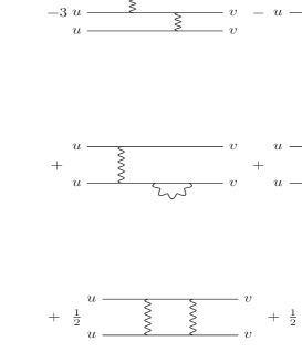
Figure 4: Expansion for the 1st order term $\mathcal{J}_{1}$. Solid lines are $y^{a}$ propagators (scalars), wavy lines represent $x_{i}$ propagators (photons and gravitons).

4.4 Implications for Our Expansion

Let us compare the new expansion $\mathcal{J}=\mathcal{J}_{0}+\mathcal{J}_{1}+\cdots$ with the old one, $\mathcal{J}=J_{0}+J_{1}+\cdots$. The first two terms of the new expansion are expressions (75) and (92). In contrast, the first two terms of the old expansion are,

$$J_{0}=1\qquad,\qquad J_{1}=i\!\mathcal{A}_{ij}\,u\Bigl{[}i\mathcal{B}\!\cdot\!iC_{i}\!\cdot\!i\mathcal{B}\!\cdot\!iC_{j}i\mathcal{B}\Bigr{]}v\;.$$ (93)

It is useful to define the difference between new and old at order $\ell$,

$$\Delta\!\mathcal{J}_{\ell}\equiv\mathcal{J}_{\ell}-J_{\ell}\;.$$ (94)

We can read off $\Delta\!\mathcal{J}_{0}$ from expression (75),

$$\Delta\!\mathcal{J}_{0}=\frac{1}{2}u\Bigl{[}i\mathcal{B}\!\cdot\!iC_{i}\!\cdot\!i\mathcal{B}\Bigr{]}v\,i\!\mathcal{A}_{ij}\,u\Bigl{[}i\mathcal{B}\!\cdot\!iC_{j}\!\cdot\!i\mathcal{B}\Bigr{]}v$$ (95)

$$\hskip 14.22636pt-\frac{3}{8}\Biggl{(}u\Bigl{[}i\mathcal{B}\!\cdot\!iC_{i}\!\cdot\!i\mathcal{B}\Bigr{]}v\,i\!\mathcal{A}_{ij}\,u\Bigl{[}i\mathcal{B}\!\cdot\!iC_{j}\!\cdot\!i\mathcal{B}\Bigr{]}v\Biggr{)}^{2}u\Bigl{[}i\mathcal{B}\!\cdot\!iC_{i}\!\cdot\!i\mathcal{B}\Bigr{]}v\,i\!\mathcal{A}_{ij}$$

$$\hskip 71.13188pt\times u\Bigl{[}i\mathcal{B}\!\cdot\!iC_{j}\!\cdot\!i\mathcal{B}\!\cdot\!iC_{k}\!\cdot\!i\mathcal{B}\Bigr{]}v\,i\!\mathcal{A}_{k\ell}\,u\Bigl{[}i\mathcal{B}\!\cdot\!iC_{\ell}\!\cdot\!i\mathcal{B}\Bigr{]}v+O(C^{6})\;.\qquad$$

Note that each contribution to $\Delta\!\mathcal{J}_{0}$ is a “tree diagram”; the expansion in powers of the interaction $C$ could also be viewed as an expansion in numbers of external lines. From expression (92) we see that $\Delta\!\mathcal{J}_{1}$ possesses both “tree” and “one loop” contributions,

$$\Delta\!\mathcal{J}_{1}^{0}=-\frac{1}{2}u\Bigl{[}i\mathcal{B}\!\cdot\!iC_{i}\!\cdot\!i\mathcal{B}\Bigr{]}v\,i\!\mathcal{A}_{ij}\,u\Bigl{[}i\mathcal{B}\!\cdot\!iC_{j}\!\cdot\!i\mathcal{B}\Bigr{]}v$$ (96)

$$\hskip 14.22636pt+\frac{7}{8}\Biggl{(}u\Bigl{[}i\mathcal{B}\!\cdot\!iC_{i}\!\cdot\!i\mathcal{B}\Bigr{]}v\,i\!\mathcal{A}_{ij}\,u\Bigl{[}i\mathcal{B}\!\cdot\!iC_{j}\!\cdot\!i\mathcal{B}\Bigr{]}v\Biggr{)}^{2}-3u\Bigl{[}i\mathcal{B}\!\cdot\!iC_{i}\!\cdot\!i\mathcal{B}\Bigr{]}v\,i\!\mathcal{A}_{ij}$$

$$\hskip 71.13188pt\times u\Bigl{[}i\mathcal{B}\!\cdot\!iC_{j}\!\cdot\!i\mathcal{B}\!\cdot\!iC_{k}\!\cdot\!i\mathcal{B}\Bigr{]}v\,i\!\mathcal{A}_{k\ell}\,u\Bigl{[}i\mathcal{B}\!\cdot\!iC_{\ell}\!\cdot\!i\mathcal{B}\Bigr{]}v+O(C^{6})\;,\qquad$$

$$\Delta\!\mathcal{J}_{1}^{1}=-u\Bigl{[}i\mathcal{B}\!\cdot\!iC_{i}\!\cdot\!i\mathcal{B}\Bigr{]}vi\!\mathcal{A}_{ij}\,u\Bigl{[}i\mathcal{B}\!\cdot\!iC_{j}\!\cdot\!i\mathcal{B}\Bigr{]}v\,i\!\mathcal{A}_{k\ell}\,u\Bigl{[}i\mathcal{B}\!\cdot\!iC_{k}\!\cdot\!i\mathcal{B}\!\cdot\!iC_{\ell}\!\cdot\!i\mathcal{B}\Bigr{]}v$$ (97)

$$+u\Bigl{[}i\mathcal{B}\!\cdot\!C_{i}\!\cdot\!i\mathcal{B}\Bigr{]}v\,i\!\mathcal{A}_{ij}\,i\!\mathcal{A}_{k\ell}\,u\Biggl{[}i\mathcal{B}\Biggr{(}\!iC_{j}\!\cdot\!i\mathcal{B}\!\cdot\!iC_{k}\!\cdot\!i\mathcal{B}\!\cdot\!iC_{\ell}\!+\!iC_{k}\!\cdot\!i\mathcal{B}\!\cdot\!iC_{j}\!\cdot\!i\mathcal{B}\!\cdot\!iC_{\ell}$$

$$+iC_{k}\!\cdot\!i\mathcal{B}\!\cdot\!iC_{\ell}\!\cdot\!i\mathcal{B}\!\cdot\!iC_{j}\!\Biggr{)}i\mathcal{B}\Biggr{]}v+\frac{1}{2}i\!\mathcal{A}_{ij}\,u\Bigl{[}i\mathcal{B}\!\cdot\!iC_{j}\!\cdot\!i\mathcal{B}\!\cdot\!iC_{k}\!\cdot\!i\mathcal{B}\Bigr{]}v\,i\!\mathcal{A}_{k\ell}\,u\Bigl{[}i\mathcal{B}\Bigl{(}iC_{\ell}$$

$$\times i\mathcal{B}\!\cdot\!iC_{i}+iC_{i}\!\cdot\!i\mathcal{B}\!\cdot\!iC_{\ell}\Bigr{)}i\mathcal{B}\Bigr{]}v\!+\!\frac{1}{2}\Biggl{(}i\!\mathcal{A}_{ij}\,u\Bigl{[}i\mathcal{B}\!\cdot\!iC_{i}\!\cdot\!i\mathcal{B}\!\cdot\!iC_{j}\!\cdot\!i\mathcal{B}\Bigr{]}v\Biggr{)}^{\!2}\!\!+O(C^{6})\;.\qquad$$

Note that the order $C^{2}$ contributions to $\Delta\!\mathcal{J}_{0}$ and $\Delta\!\mathcal{J}_{1}^{0}$ cancel. They do not cancel at order $C^{4}$, but the residual $C^{4}$ terms are canceled by $\Delta\!\mathcal{J}_{2}^{0}$. So the new expansion does not move the old diagrams from one order to another, rather it adds a new class of diagrams — with more external lines — to one order and subtracts them from higher orders. What we have learned can be summarized by the following observations:

• Each term $\mathcal{J}_{\ell}$ in the new expansion can be written as an infinite series which begins at order $C^{2\ell}$;

• The lowest order term in this series expansion of each $\mathcal{J}_{\ell}$ is the old $\ell$-loop term $J_{\ell}$;

• The new terms in $\mathcal{J}_{\ell}$ involve diagrams with up to and including $\ell$ loops;

• The new terms at each order have more powers of the external state factors $u^{a}$ and $v^{b}$; and

• The sum of all the new terms is zero.

Although there is no guarantee that the new expansion is free of ultraviolet divergences, it does possess a number of desirable features. Note first that ultraviolet divergences are no worse in the new expansion than the old one because none of the new diagrams in $\mathcal{J}_{\ell}$ have more than $\ell$ loops. Our simple model makes no distinction between photons and gravitons but the quantum field theoretic expansion will of course involve both particles. The new diagrams — with more powers of the coupling constants $e^{2}$ and $G$, but no more loops — are one way gravity at order $\ell$ in the new expansion can know about an order $\ell$ divergence from the gauge sector. So the new expansion breaks the conundrum of conventional perturbation theory that the gravitational response to a problem at one order cannot come until the next order. Note finally, that the infinite sums of new diagrams at any fixed order of the new expansion allow the possibility of getting nonanalytic dependence upon $G$ and $e^{2}$.

5 The 0th Order Term

The purpose of this section is the evaluate the 0th order term in the new expansion of expression (49) for the scalar mass. Recall that this means solving the problem of a first quantized Klein-Gordon scalar which forms a bound state in the gravitational and electrostatic potentials sourced by its own probability current. We begin by specializing the Lagrangians, the field equations and the normalization condition to the bound state ansatz (59-61). We then note that one of the equations can be solved exactly for the negative energy gravitational degree of freedom. Substituting this solution into the action gives a functional of the remaining fields whose minimization yields the remaining field equations. This functional serves as the basis for a variational formulation of the problem. The section closes with a numerical solution.

5.1 Field Equations

If a bound state forms we can simplify the fields to take the form (59-61),

$$\phi=e^{-iEt}F(r)\qquad,\qquad A_{\mu}=-\Phi(r)\delta^{0}_{\mu}\;,$$ (98)

$$g_{00}=-B(r)\qquad,\qquad g_{0i}=0\qquad,\qquad g_{ij}=\pi_{ij}+\widehat{r}_{i}\widehat{r}_{j}A(r)\;.$$ (99)

Here $\widehat{r}_{i}\equiv x_{i}/r$ is the radial unit vector and $\pi_{ij}\equiv\delta_{ij}-\widehat{r}_{i}\widehat{r}_{j}$ is the transverse projection operator. The nonvanishing components of the affine connection are,

$$\Gamma^{0}_{~{}0i}=\widehat{r}_{i}\Bigl{(}\frac{B^{\prime}}{2B}\Bigr{)}\quad,\quad\Gamma^{i}_{~{}00}=\widehat{r}_{i}\Bigl{(}\frac{B^{\prime}}{2A}\Bigr{)}\quad,\quad\Gamma^{i}_{~{}jk}=\widehat{r}_{i}\widehat{r}_{j}\widehat{r}_{k}\frac{A^{\prime}}{2A}\!+\!\widehat{r}_{i}\pi_{jk}\Bigl{(}\frac{A\!-\!1}{rA}\Bigr{)}\;.$$ (100)

The nonzero components of the Riemann tensor are,

$$R^{0}_{~{}i0j} = \widehat{r}_{i}\widehat{r}_{j}\Bigl{[}-\frac{B^{\prime\prime}}{2B}\!+\!\frac{{B^{\prime}}^{2}}{4B^{2}}\!+\!\frac{A^{\prime}B^{\prime}}{4AB}\Bigr{]}-\pi_{ij}\Bigl{(}\frac{B^{\prime}}{2rAB}\Bigr{)}\;,\qquad$$ (101)

$$R^{i}_{~{}jk\ell} = \Bigl{[}\pi_{ik}\widehat{r}_{j}\widehat{r}_{\ell}\!-\!\pi_{i\ell}\widehat{r}_{j}\widehat{r}_{k}\Bigr{]}\Bigl{(}\frac{A^{\prime}}{2rA}\Bigr{)}+\Bigl{[}\pi_{i\ell}\widehat{r}_{i}\widehat{r}_{k}\!-\!\pi_{jk}\widehat{r}_{i}\widehat{r}_{\ell}\Bigr{]}\Bigl{(}\frac{A^{\prime}}{2rA^{2}}\Bigr{)}\qquad$$ (102)

$$\hskip 170.71652pt+\Bigl{[}\pi_{ik}\pi_{j\ell}\!-\!\pi_{i\ell}\pi_{jk}\Bigr{]}\Bigl{(}\frac{A\!-\!1}{r^{2}A}\Bigr{)}\;.\qquad$$

Contraction gives the Ricci tensor $R_{\mu\nu}=R^{\rho}_{~{}\mu\rho\nu}$,

$$R_{00} = \frac{B^{\prime\prime}}{2A}\!-\!\frac{{B^{\prime}}^{2}}{4AB}\!-\!\frac{A^{\prime}B^{\prime}}{4A^{2}}\!+\!\frac{A^{\prime}}{rA}\;,\qquad$$ (103)

$$R_{ij} = \widehat{r}_{i}\widehat{r}_{j}\Bigl{[}-\frac{B^{\prime\prime}}{2B}\!+\!\frac{{B^{\prime}}^{2}}{4B^{2}}\!+\!\frac{A^{\prime}B^{\prime}}{4AB}\!+\!\frac{A^{\prime}}{rA}\Bigr{]}$$ (104)

$$\hskip 128.0374pt+\pi_{ij}\Bigl{[}-\frac{B^{\prime}}{2rAB}\!+\!\frac{A^{\prime}}{2rA^{2}}+\Bigl{(}\frac{A\!-\!1}{r^{2}A}\Bigr{)}\Bigr{]}\;.\qquad$$

And contracting that gives the Ricci scalar $R=g^{\mu\nu}R_{\mu\nu}$,

$$R=-\frac{B^{\prime\prime}}{AB}\!+\!\frac{{B^{\prime}}^{2}}{2AB^{2}}\!+\!\frac{A^{\prime}B^{\prime}}{2A^{2}B}\!+\!\frac{2A^{\prime}}{rA^{2}}\!-\!\frac{2B^{\prime}}{rAB}\!+\!2\Bigl{(}\frac{A\!-\!1}{r^{2}A}\Bigr{)}\;.$$ (105)

In specializing the various Lagrangians (15-17) to our ansatz (98-99) it is best to use spherical coordinates and integrate the angles so that the effective measure factor is,

$$\sqrt{-g}=4\pi r^{2}\sqrt{A(r)B(r)}\;.$$ (106)

ADM long ago worked out the surface term one must add to the Hilbert Lagrangian (15) for asymptotically flat field configurations [22]. For our static, spherically symmetric geometry the result is,

$$\mathcal{L}_{\rm ADM}\longrightarrow\frac{1}{16\pi G}\Biggl{[}R\sqrt{-g}-\frac{\partial}{\partial r}\Bigl{(}\frac{B^{\prime}\sqrt{-g}}{AB}\Bigr{)}\Biggr{]}=\frac{1}{8\pi G}\Biggl{[}\frac{A^{\prime}}{rA^{2}}\!+\!\Bigl{(}\frac{A\!-\!1}{r^{2}A}\Bigr{)}\Biggr{]}\sqrt{-g}\;.$$ (107)

The other two Lagrangians (16-17) require no surface terms,

$$\mathcal{L}_{\rm EM} \longrightarrow \frac{\epsilon_{0}{\Phi^{\prime}}^{2}}{2AB}\sqrt{-g}\;,\qquad$$ (108)

$$\mathcal{L}_{\rm SC} \longrightarrow \frac{1}{B}(E\!+\!e\Phi)^{2}F^{2}\sqrt{-g}-\frac{1}{A}{F^{\prime}}^{2}\sqrt{-g}-M_{0}^{2}F^{2}\sqrt{-g}\;.\qquad$$ (109)

Hence the action is,

$$S[F,\Phi,B,A]=(t_{+}\!-\!t_{-})\int_{0}^{\infty}\!\!dr\,\sqrt{-g}\,\Biggl{\{}\frac{1}{8\pi G}\Biggl{[}\frac{A^{\prime}}{rA^{2}}\!+\!\Bigl{(}\frac{A\!-\!1}{r^{2}A}\Bigr{)}\Biggr{]}$$ (110)

$$\hskip 128.0374pt+\frac{\epsilon_{0}{\Phi^{\prime}}^{2}}{2AB}+\frac{(E\!+\!e\Phi)^{2}F^{2}}{B}-\frac{{F^{\prime}}^{2}}{A}-M_{0}^{2}F^{2}\Biggr{\}}.\qquad$$

It is well known that the operation of making an ansatz for the solution does not commute with varying the action to obtain the field equations. The correct procedure is to vary first and then simplify. However, all of the equations one gets by simplifying first and then varying are correct, and it turns out that the only ones we miss are the trivial relations implied by the Bianchi identity [23]. Except for the overall factor of $\Delta t\equiv(t_{+}-t_{-})$, the variations with respect to various fields are,

$$\frac{1}{\Delta t}\frac{\delta S}{\delta F} = \frac{\partial}{\partial r}\Biggl{[}\frac{2F^{\prime}\sqrt{-g}}{A}\Biggr{]}+\frac{2(E\!+\!e\Phi)^{2}F\sqrt{-g}}{B}-2M_{0}^{2}F\sqrt{-g}\;,\qquad$$ (111)

$$\frac{1}{\Delta t}\frac{\delta S}{\delta\Phi} = \frac{\partial}{\partial r}\Biggl{[}\frac{\epsilon_{0}\Phi^{\prime}\sqrt{-g}}{AB}\Biggr{]}+\frac{2e(E\!+\!e\Phi)F^{2}\sqrt{-g}}{B}\;,\qquad$$ (112)

$$\frac{1}{\Delta t}\frac{\delta S}{\delta B} = \Biggl{\{}\frac{1}{8\pi G}\Biggl{[}\frac{A^{\prime}}{rA^{2}}\!+\!\Bigl{(}\frac{A\!-\!1}{r^{2}A}\Bigr{)}\Biggr{]}-\frac{\epsilon_{0}{\Phi^{\prime}}^{2}}{2AB}$$ (113)

$$\hskip 99.58464pt-\frac{(E\!+\!e\Phi)^{2}F^{2}}{B}-\frac{{F^{\prime}}^{2}}{A}-M_{0}^{2}F^{2}\Biggr{\}}\frac{\sqrt{-g}}{2B}\;,\qquad$$

$$\frac{1}{\Delta t}\frac{\delta S}{\delta A} = \Biggl{\{}\frac{1}{8\pi G}\Biggl{[}-\frac{B^{\prime}}{rAB}\!+\!\Bigl{(}\frac{A\!-\!1}{r^{2}A}\Bigr{)}\Biggr{]}-\frac{\epsilon_{0}{\Phi^{\prime}}^{2}}{2AB}$$ (114)

$$\hskip 99.58464pt+\frac{(E\!+\!e\Phi)^{2}F^{2}}{B}+\frac{{F^{\prime}}^{2}}{A}-M_{0}^{2}F^{2}\Biggr{\}}\frac{\sqrt{-g}}{2A}\;.\qquad$$

Our goal is to find $F(r)$, $\Phi(r)$, $B(r)$ and $A(r)$ so as to make each of the variations (111-114) vanish. However, those equations have solutions for any constant $E$. As always, it is normalizability which puts the “quantum” in quantum mechanics. For our problem the normalization condition is,

$$2\int_{0}^{\infty}\!\!dr\sqrt{-g}\,\frac{(E\!+\!e\Phi)F^{2}}{B}=1\;.$$ (115)

Any field configurations $F_{0}(r)$, $\Phi_{0}(r)$, $B_{0}(r)$ and $A_{0}(r)$ which make all the variations (111-114) vanish and also obey (115) will only do so for very special values of $E$. Note that the field equations and normalizability requires $A(r)$ to approach one at infinity, and $F(r)$ to approach zero. The asymptotic values of $\Phi(r)$ and $B(r)$ are both gauge choices. By choosing the $U(1)$ gauge parameter to be $-t\times\Phi_{\infty}$ we can make $\Phi(r)$ vanish at infinity. By changing time to $t/k$ we induce the rescalings,

$$B(r) \longrightarrow k^{2}\times B(r)\;,$$ (116)

$$\Phi(r) \longrightarrow k\times\Phi(r)\;,$$ (117)

$$E \longrightarrow k\times E\;.$$ (118)

We shall always use this freedom to make $B(r)$ approach one at infinity.

If we can find a normalized solution $F_{0}(r)$, $\Phi_{0}(r)$, $B_{0}(r)$ and $A_{0}(r)$ then our zeroth order result for the mass is,

$$M_{\rm 0th}=E-\frac{1}{\Delta t}S[F_{0},\Phi_{0},B_{0},A_{0}]\;.$$ (119)

The first term on the right hand side of (119) is from the the two scalar fields,

$$\phi(t_{+},\vec{x})\phi^{*}(t_{-},\vec{0})\longrightarrow F_{0}(r)F_{0}(0)e^{-iE\Delta t}\;.$$ (120)

The final term in (119) represents the gravitational and electromagnetic contribution to the mass. Note that the scalar action vanishes for solutions because the scalar Lagrangian is a surface term which goes to zero,

$$\mathcal{L}_{\rm SC}\longrightarrow-\frac{\partial}{\partial r}\Biggl{[}\frac{F_{0}F_{0}^{\prime}\sqrt{-g_{0}}}{A_{0}}\Biggr{]}\;.$$ (121)

5.2 A Variational Formalism

Solving differential equations is tough, and we are not able to find exact solutions for all four of the fields. For many bound state problems in quantum mechanics the absence of exact solutions is not crippling because variational techniques allow one to derive strong bounds on the ground state energy. Such a technique would be simple to formulate for our Klein-Gordon scalar if only the electromagnetic and gravitational potentials were fixed. However, the fact that these potentials are sourced by the Klein-Gordon wave function itself endows this problem with a slippery, nonlinear character. The presence of gravitational interactions is especially problematic because some of the constrained degrees of freedom in gravity possess negative energy. Instability is only avoided by constraining these degrees of freedom to obey their field equations; attempting to minimize the action with respect to these degrees of freedom would carry one away from the actual solution.

There are good reasons for suspecting that the field $B(r)$ is the only negative energy degree of freedom. In the normal ADM formalism $B=N^{2}$ would be the square of the lapse field, and it could be specified arbitrarily as a choice of gauge. However, $B$ is a dynamical degree of freedom in this problem. The structure of our Lagrangian is similar to the usual formalism for describing cosmological perturbations during primordial inflation [24]. In that setting, as for us, the Lagrangian can be written as the sum of a “kinetic” part $K$ and a “potential” part $P$,

$$\mathcal{L}=\Biggl{[}\frac{K}{B}+P\Biggr{]}\sqrt{-g}\;.$$ (122)

For us the kinetic and potential parts are,

$$K = \frac{\epsilon_{0}{\Phi^{\prime}}^{2}}{2A}+(E\!+\!e\Phi)^{2}F^{2}\;,\qquad$$ (123)

$$P = \frac{1}{8\pi G}\Biggl{[}\frac{A^{\prime}}{rA^{2}}\!+\!\Bigl{(}\frac{A\!-\!1}{r^{2}A}\Bigr{)}\Biggr{]}-\frac{{F^{\prime}}^{2}}{A}-M_{0}^{2}F^{2}\;.\qquad$$ (124)

The field equation for $B$ is algebraic and has a trivial solution,

$$\frac{1}{\Delta t}\frac{\delta S}{\delta B}=\Biggl{[}-\frac{K}{B}+P\Biggr{]}\frac{\sqrt{-g}}{2B}=0\qquad\Longrightarrow\qquad B=\frac{K}{P}\;.$$ (125)

Substituting (125) into (122) allows us to express the action in terms of just $F(r)$, $\Phi(r)$ and $A(r)$,

$$S[F,\Phi,A]=8\pi\Delta t\int_{0}^{\infty}\!\!dr\,r^{2}\sqrt{AKP}\;.$$ (126)

It is simple to show that varying (126) gives equations (111-112) and (114). Because (126) is positive semi-definite, the problem of extremizing it is likely to be the same as that of minimizing it. The corresponding normalization condition is,

$$8\pi\int_{0}^{\infty}\!\!dr\,r^{2}\sqrt{\frac{AK}{P}}\,(E\!+\!e\Phi)F^{2}=1\;.$$ (127)

And our zeroth order result for the scalar mass becomes,

$$M_{\rm 0th}=E-8\pi\int_{0}^{\infty}\!\!dr\,r^{2}\sqrt{A_{0}K_{0}P_{0}}\;.$$ (128)

We illustrate the method with simple trial functions for $F(r)$, $\Phi(r)$ and $A(r)$. We cannot make $F(r)$ a spherical shell like ADM, or even a hard sphere, because the factors of ${F^{\prime}}^{2}$ become ill-defined if $F(r)$ has a discontinuity. The next best thing is to assume the scalar drops linearly to zero within some distance $R$,

$$F(r)=a(R\!-\!r)\theta(R\!-\!r)\;.$$ (129)

Comparably simple forms for the potentials are,

$$\Phi(r) = -\frac{e\theta(R\!-\!r)}{4\pi\epsilon_{0}R}-\frac{e\theta(r\!-\!R)}{4\pi\epsilon_{0}r}\;,\qquad$$ (130)

$$\frac{1}{A(r)} = \Bigl{[}1\!-\!br^{2}\Bigr{]}\theta(R\!-\!r)+\Bigl{[}1\!-\!\frac{c}{r}\!+\!\frac{d}{r^{2}}\Bigr{]}\theta(r\!-\!R)\;.\qquad$$ (131)

We can make $A(r)$ continuous by choosing,

$$b=\frac{c}{R^{3}}-\frac{d}{R^{4}}\;.$$ (132)

The corresponding forms for the kinetic and potential terms are,

$$K(r) = \Bigl{(}E\!-\!\frac{\alpha}{R}\Bigr{)}^{2}a^{2}(R\!-\!r)^{2}\theta(R\!-\!r)+\frac{\alpha}{8\pi r^{4}}\Bigl{(}1\!-\!\frac{c}{r}\!+\!\frac{d}{r^{2}}\Bigr{)}\theta(r\!-\!R)\;,\qquad$$ (133)

$$P(r) = \Biggl{[}\frac{3b}{8\pi G}-a^{2}\Bigl{[}1\!-\!br^{2}\!+\!M_{0}^{2}(R\!-\!r)^{2}\Bigr{]}\Biggr{]}\theta(R\!-\!r)+\frac{d\theta(r\!-\!R)}{8\pi Gr^{4}}\;.\qquad$$ (134)

Hence the potential $B(r)$ is,

$$B(r)=\frac{(E\!-\!\frac{\alpha}{R})^{2}a^{2}(R\!-\!r)^{2}\theta(R\!-\!r)}{\frac{3b}{8\pi G}-a^{2}[1\!-\!br^{2}\!+\!M_{0}^{2}(R\!-\!r)^{2}]}+\frac{\frac{\alpha}{8\pi r^{4}}(1\!-\!\frac{c}{r}\!+\!\frac{d}{r^{2}})\theta(r\!-\!R)}{\frac{d}{8\pi Gr^{4}}}\;.$$ (135)

Enforcing that $B(r)$ goes to one at infinity determines the coefficient $d$,

$$d=\alpha G\;,$$ (136)

where $\alpha\equiv e^{2}/4\pi\epsilon_{0}\approx 1/137$ is the fine structure constant. Enforcing continuity at $r=R$ — which means $B(R)=0$ — requires the choice,

$$c=R+\frac{\alpha G}{R}\qquad\Longrightarrow\qquad b=\frac{1}{R^{2}}\;.$$ (137)

At this stage the free parameters in our trial solution are $R$, $a$ and the energy $E$. The next step is to enforce normalizability, which requires,

$$\frac{1}{8\pi} = \int_{0}^{R}\!\!\frac{dr\,r^{2}}{\sqrt{1\!-\!br^{2}}}\frac{(E\!-\!\frac{\alpha}{R})^{2}a^{3}(R\!-\!r)^{3}}{\sqrt{\frac{3b}{8\pi G}\!-\!a^{2}[1\!-\!br^{2}\!+\!M_{0}^{2}(R\!-\!r)^{2}]}}\;,\qquad$$ (138)

$$= (RE\!-\!\alpha)^{2}R^{4}a^{2}\int_{0}^{1}\!\!\frac{dx\,x^{2}}{\sqrt{1\!-\!x^{2}}}\frac{(1\!-\!x)^{3}}{\sqrt{\frac{3}{8\pi GR^{2}a^{2}}\!-\![1\!-\!x^{2}\!+\!R^{2}M_{0}^{2}(1\!-\!x)^{2}]}}\;,\qquad$$ (139)

$$\equiv (RE\!-\!\alpha)^{2}R^{4}a^{2}\times I\Bigl{(}GR^{2}a^{2},R^{2}M_{0}^{2})\;.\qquad$$ (140)

The function $I(x,y)$ in equation (140) can be expressed in terms of elliptic integrals but we may as well treat it as an elementary function and use it to express the energy,

$$E=\Biggl{[}\frac{1}{\sqrt{8\pi R^{4}a^{2}I(GR^{2}a^{2},R^{2}M_{0}^{2})}}+\alpha\Biggr{]}\frac{1}{R}\;.$$ (141)

We can now regard the two free parameters as,

$$A\equiv\frac{Ra}{M_{0}}\qquad,\qquad\mu\equiv RM_{0}\;.$$ (142)

The field action is,

$$\frac{S}{\Delta t}=\Biggl{[}\frac{\sqrt{8\pi}\,AJ(GM_{0}^{2}A^{2},\mu^{2})}{\sqrt{I(GM_{0}^{2}A^{2},\mu^{2})}}+\frac{\alpha}{\mu}\Biggr{]}M_{0}\;,$$ (143)

where the new integral is,

$$J(GM_{0}^{2}A^{2},\mu^{2})\equiv\int_{0}^{1}\!\frac{dx\,x^{2}(1\!-\!x)}{\sqrt{1\!-\!x^{2}}}\sqrt{\frac{3}{8\pi GM_{0}^{2}A^{2}}\!-\![1\!-\!x^{2}\!+\!\mu^{2}(1\!-\!x)^{2}]}\;.$$ (144)

We determine the free parameters $A$ and $\mu$ by minimizing $S/\Delta t$.

Expressions (140), (143) and (144) seem very complicated. However, note that because $I(GM_{0}^{2}A^{2},\mu^{2})$ is an increasing function of $A$ and $\mu$, and $J(GM_{0}^{2}A^{2},\mu^{2})$ is a decreasing function of $A$ and $\mu$, $S/\Delta t$ is a decreasing function of $\mu$ at fixed $A$. Hence $S/\Delta t$ is minimized, at fixed $A$, by choosing $\mu$ to be the maximum value for which the two integrals remain real,

$$\mu_{\rm max}=\sqrt{\frac{3}{8\pi GM_{0}^{2}A^{2}}\!-\!1}\qquad\Longrightarrow\qquad 0<A<A_{\rm max}=\sqrt{\frac{3}{8\pi GM_{0}^{2}}}\;.$$ (145)

At $\mu=\mu_{\rm max}$ the two integrals become,

$$i(\mu_{\rm max}) \equiv I(GM_{0}^{2}A^{2},\mu_{\rm max}^{2})=\int_{0}^{1}\!\!\frac{dx\,x^{2}}{\sqrt{1\!-\!x^{2}}}\frac{(1\!-\!x)^{3}}{\sqrt{\mu_{\rm max}^{2}[1\!-\!(1\!-\!x)^{2}]\!+\!x^{2}}}\;,\qquad$$ (146)

$$j(\mu_{\rm max}) \equiv J(GM_{0}^{2}A^{2},\mu_{\rm max}^{2})=\int_{0}^{1}\!\frac{dx\,x^{2}(1\!-\!x)}{\sqrt{1\!-\!x^{2}}}\sqrt{\mu_{\rm max}^{2}[1\!-\!(1\!-\!x)^{2}]\!+\!x^{2}}\;.\qquad$$ (147)

And the field action (143) takes the form,

$$\frac{S}{\Delta t}=\Biggl{[}\sqrt{\frac{3}{GM_{0}^{2}}}\,\frac{j(\mu_{\rm max})}{\sqrt{(1\!+\!\mu_{\rm max}^{2})i(\mu_{\rm max})}}+\frac{\alpha}{\mu_{\rm max}}\Biggr{]}M_{0}\;.$$ (148)

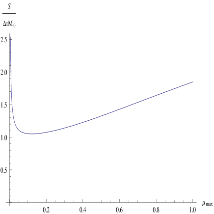
Figure 5: Plot of $\frac{S}{M_{0}\Delta t}$ versus $\mu_{\rm max}$ from equation (148) for $GM_{0}^{2}=0.36$. The minimum seems to be at about $\mu_{\rm max}=0.12$.

At this stage the problem is numerical. Fig. 5 shows $S/M_{0}\Delta t$ as a function of $\mu_{\rm max}$ for $GM_{0}^{2}=0.36$. The minimum seems to be at about $\mu_{\rm max}=0.12$, which corresponds to,

$$R = \frac{\mu_{\rm max}}{\sqrt{GM_{0}^{2}}}\times\sqrt{G}\approx 0.20\times\sqrt{G}\;,\qquad$$ (149)

$$a = \sqrt{\frac{3GM_{0}^{2}}{8\pi}}\frac{1}{\mu_{\rm max}\sqrt{1\!+\!\mu_{\rm max}^{2}}}\times\frac{1}{G}\approx 1.7\times\frac{1}{G}\;,\qquad$$ (150)

$$E = \Biggl{[}\frac{GM_{0}^{2}}{\mu_{\rm max}^{2}}\sqrt{\frac{1\!+\!\mu_{\rm max}^{2}}{3i(\mu_{\rm max})}}\!+\!\frac{\alpha\sqrt{GM_{0}^{2}}}{\mu_{\rm max}}\Biggr{]}\frac{1}{\sqrt{G}}\approx 62\times\frac{1}{\sqrt{G}}\;,$$ (151)

$$M = E-\frac{S}{\Delta t}\approx 62\times\frac{1}{\sqrt{G}}\;.\qquad$$ (152)

We will see that these results are not very accurate.

5.3 Numerical Results

It is desirable to check any variational ansatz against a direct, numerical solution to the problem. Of course computers can only solve for dimensionless quantities, so it is first necessary to express everything in geometrodynamical units, using $G$ to absorb each quantity’s natural units,

$$r=\sqrt{G}\,\widetilde{r}\;\;,\;\;M_{0}=\frac{\widetilde{M}}{\sqrt{G}}\;\;,\;\;E=\frac{\widetilde{E}}{\sqrt{G}}\;\;,\;\;M=\frac{\widetilde{M}}{\sqrt{G}}\;\;,$$ (153)

$$F(r)=\frac{\widetilde{F}(\widetilde{r})}{\sqrt{G}}\;\;,\;\;\Phi(r)=\frac{[\widetilde{\Phi}(\widetilde{r})\!-\!\widetilde{E}]}{e\sqrt{G}}\;\;,\;\;B(r)=\widetilde{B}(\widetilde{r})\;\;,\;\;A(r)=\widetilde{A}(\widetilde{r})\;\;,$$ (154)

$$\sqrt{-g(r)}=G\sqrt{-\widetilde{g}(\widetilde{r})}\;\;,\;\;K(r)=\frac{\widetilde{K}(\widetilde{r})}{G^{2}}\;\;,\;\;P(r)=\frac{\widetilde{P}(\widetilde{r})}{G^{2}}\;\;.$$ (155)

Note that we have absorbed the energy into the electrostatic potential. In all cases we employ a tilde to denote the dimensionless quantity. Geometrodynamic fields such as $\widetilde{F}$ are considered to be functions of the geometrodynamic radius $\widetilde{r}$. A prime on such a field indicates differentiation with respect to $\widetilde{r}$, so we have,

$$F^{\prime}=\frac{\widetilde{F}^{\prime}}{G}\qquad,\qquad\Phi^{\prime}=\frac{\widetilde{\Phi}^{\prime}}{eG}\;.$$ (156)

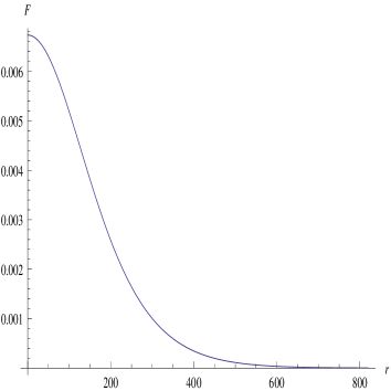
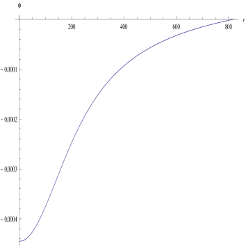
Figure 6: Plots of the scalar amplitude $F(r)$ (in units of $M_{\rm Pl}=1/\sqrt{G}$) and the electrostatic potential $\Phi(r)$ (in units of $M_{\rm Pl}/e$) as functions of $r$ (in units of $1/M_{\rm Pl}$). These figures were generated for bare mass $M_{0}=0.60\,M_{\rm Pl}$.

In these units the four field equations (111-114) take the form,

$$\frac{\partial}{\partial\widetilde{r}}\Biggl{[}\frac{\widetilde{F}^{\prime}\sqrt{-\widetilde{g}}}{\widetilde{A}}\Biggr{]}+\frac{\widetilde{\Phi}^{2}\widetilde{F}\sqrt{-\widetilde{g}}}{\widetilde{B}}-\widetilde{M}_{0}^{2}\widetilde{F}\sqrt{-\widetilde{g}}=0\;,\qquad$$ (157)

$$\frac{\partial}{\partial\widetilde{r}}\Biggl{[}\frac{\widetilde{\Phi}^{\prime}\sqrt{-\widetilde{g}}}{\widetilde{A}\widetilde{B}}\Biggr{]}+\frac{8\pi\alpha\widetilde{\Phi}\widetilde{F}^{2}\sqrt{-\widetilde{g}}}{\widetilde{B}}=0\;,\qquad$$ (158)

$$\frac{1}{8\pi}\Biggl{[}\frac{\widetilde{A}^{\prime}}{\widetilde{r}\widetilde{A}^{2}}\!+\!\Bigl{(}\frac{\widetilde{A}\!-\!1}{\widetilde{r}^{2}\widetilde{A}}\Bigr{)}\Biggr{]}-\frac{\widetilde{\Phi}^{\prime 2}}{8\pi\alpha\widetilde{A}\widetilde{B}}-\frac{\widetilde{\Phi}^{2}\widetilde{F}^{2}}{\widetilde{B}}-\frac{\widetilde{F}^{\prime 2}}{\widetilde{A}}-\widetilde{M}_{0}^{2}\widetilde{F}^{2}=0\;,\qquad$$ (159)

$$\frac{1}{8\pi}\Biggl{[}-\frac{\widetilde{B}^{\prime}}{\widetilde{r}\widetilde{A}\widetilde{B}}\!+\!\Bigl{(}\frac{\widetilde{A}\!-\!1}{\widetilde{r}^{2}\widetilde{A}}\Bigr{)}\Biggr{]}-\frac{\widetilde{\Phi}^{\prime 2}}{8\pi\alpha\widetilde{A}\widetilde{B}}+\frac{\widetilde{\Phi}^{2}\widetilde{F}^{2}}{\widetilde{B}}+\frac{\widetilde{F}^{\prime 2}}{\widetilde{A}}-\widetilde{M}_{0}^{2}\widetilde{F}^{2}=0\;.\qquad$$ (160)

(Recall that $\alpha\equiv e^{2}/4\pi\epsilon_{0}\approx 1/137$ is the fine structure constant.) The kinetic and potential terms are,

$$\widetilde{K} = \frac{\widetilde{\Phi}^{\prime 2}}{8\pi\alpha\widetilde{A}}+\widetilde{\Phi}^{2}\widetilde{F}^{2}\;,\qquad$$ (161)

$$\widetilde{P} = \frac{1}{8\pi}\Biggl{[}\frac{\widetilde{A}^{\prime}}{\widetilde{r}\widetilde{A}^{\prime 2}}\!+\!\Bigl{(}\frac{\widetilde{A}\!-\!1}{\widetilde{r}^{2}\widetilde{A}}\Bigr{)}\Biggr{]}-\frac{\widetilde{F}^{\prime 2}}{\widetilde{A}}-\widetilde{M}_{0}^{2}\widetilde{F}^{2}\;.\qquad$$ (162)

The normalization condition is,

$$2\int_{0}^{\infty}\!\!d\widetilde{r}\sqrt{-\widetilde{g}}\,\frac{\widetilde{\Phi}\widetilde{F}^{2}}{\widetilde{B}}=1\;.$$ (163)

And the final result is,

$$\widetilde{M}_{\rm 0th}=\widetilde{E}-8\pi\int_{0}^{\infty}\!\!d\widetilde{r}\,\widetilde{r}^{2}\sqrt{\widetilde{A}\widetilde{K}\widetilde{P}}\;.$$ (164)

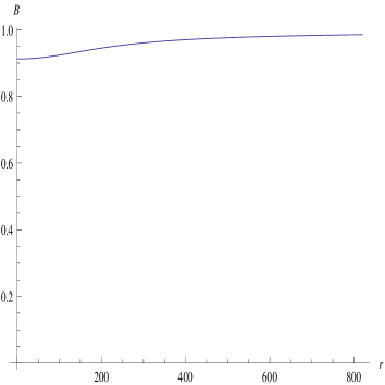
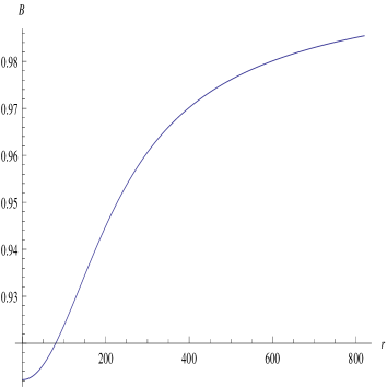
Figure 7: Plots of minus the $tt$ component of the metric $B(r)$ (dimensionless) as a function of $r$ (in units of $1/M_{\rm Pl}=\sqrt{G}$). The right hand figure has an expanded vertical axis to show the small variation of the field. These figures were generated for bare mass $M_{0}=0.60\,M_{\rm Pl}$.

The nonlinear nature of this problem requires a special solution strategy. The development of our technique was facilitated by the vast amount of work that has been done of “boson stars” [25, 26]. There has also been a recent study by Carlip of gravitationally bound atoms [27].

Our strategy is to begin by evolving equations (157-160) outward from $\widetilde{r}=0$, with arbitrary choices for $\widetilde{F}(0)>0$, $\widetilde{\Phi}(0)<0$ and $\widetilde{B}(0)>0$, and with the other boundary values at,

$$\widetilde{F}^{\prime}(0)=0\;\;,\;\;\widetilde{\Phi}(0)=0\;\;,\;\;\widetilde{A}(0)=1\;.$$ (165)

The choice of $\widetilde{B}(0)>0$ really is arbitrary because we will eventually make a global re-scaling of time to force $\widetilde{B}(\widetilde{r})$ to approach one at infinity. However, the choice of $\widetilde{\Phi}(0)$ essentially gives the energy, and this matters of course. There is zero probability of guessing a true eigenvalue. With the other conditions fixed, varying $\widetilde{\Phi}(0)$ gives solutions for which $\widetilde{F}(\widetilde{r})$ either becomes negative (which a magnitude cannot do) or grows at infinity (which a normalizable solution cannot do). One knows that a true energy eigenvalue has been bracketed between two different choices of $\widetilde{\Phi}(0)$ when the behavior of $\widetilde{F}(\widetilde{r})$ changes from one extreme to the other. Then one closes in on the eigenvalue to whatever accuracy is desired. Note that this means cutting off the behavior of the solution past a certain value of $\widetilde{r}$, beyond which $\widetilde{F}(\widetilde{r})$ begins to degenerate.

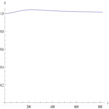
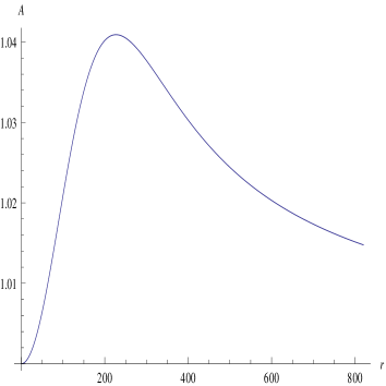
Figure 8: Plots of the $rr$ component of the metric $A(r)$ (dimensionless) as a function of $r$ (in units of $1/M_{\rm Pl}=\sqrt{G}$). The right hand figure has an expanded vertical axis to show the small variation of the field. These figures were generated for bare mass $M_{0}=0.60\,M_{\rm Pl}$.

The procedure we have just outlined gives a solution which is normalizable, but not yet normalized. For that we compute (163) and then either increase or decrease $\widetilde{F}(0)$ as needed. Of course the nonlinear nature of this problem means that one does not get a solution by simply multiplying $\widetilde{F}(\widetilde{r})$ by a constant! We must instead start from the new $\widetilde{F}(0)$ and again go through the process of trapping the energy eigenvalue. However, our evolution programs are efficient enough that this can be done to high accuracy, and fairly quickly.

Figures 6-8 show the behavior of the fields for $\widetilde{M}=0.6$. For this bare mass the energy is $\widetilde{E}\approx 0.586378$ and the total mass is $\widetilde{M}\approx-0.000882$. A measure of the numerical error is the accuracy with which the scalar action vanishes, which is $\widetilde{S}_{\rm SC}/\Delta t\approx 3\times 10^{-6}$. Another measure of accuracy comes from the finite cutoff at $\widetilde{r}=\widetilde{R}_{\rm cut}$, occasioned by the finite accuracy of $\widetilde{E}$. For that bare mass we cut the various integrations off at $\widetilde{R}_{\rm cut}=500$, which corresponds to a contribution of $\alpha/\widetilde{R}_{\rm cut}\approx 10^{-5}$ from the electromagnetic tail.

The variational results (149-152) obtained in the previous subsection are quite different from the numerical solution. From Fig. 6 one can see than the scalar amplitude has roughly the same shape as that of our trial function (129), but with initial height $Ga\approx 0.0065$, rather than the variational value (150) of $Ga\approx 1.7$. And the radial extent is about $\sqrt{G}\,R\approx 300$, rather than the variational result (149) of $\sqrt{G}\,R\approx 0.20$. There is no chance that the discrepancy derives from the numerical solution, the error of which we estimate to be no larger than $10^{-5}$. The problem must lie instead with the variational formalism. Our trial solution seems roughly correct, but it may be that, like $B(r)$, the gravitational potential $A(r)$ represents a negative energy direction in field space. In that case minimizing the constrained action would take us away from the actual solution, which seems to be what has happened.

	$\!\!\!\!\widetilde{M}_{0}\!\!\!\!$	$\!\!\!\!\widetilde{E}\!\!\!\!$	$\!\!\!\!\widetilde{M}\!\!\!\!$	$\!\!\!\!\widetilde{S}_{\rm SC}/\Delta t\!\!\!\!$	$\!\!\!\!\widetilde{R}_{\rm cut}\!\!\!\!$
	0.15	0.149994	-0.000320	$2.0\times 10^{-10}$	70,000
	0.20	0.199962	-0.000260	$1.5\times 10^{-9}$	25,000
	0.25	0.249870	-0.000505	$2.9\times 10^{-9}$	11,750
	0.30	0.299653	-0.000239	$9.6\times 10^{-9}$	4,500
	0.35	0.349215	-0.001075	$5.7\times 10^{-8}$	3,200
	0.40	0.398424	-0.000455	$1.3\times 10^{-7}$	1,800
	0.45	0.447073	-0.000826	$3.5\times 10^{-7}$	1,300
	0.50	0.494904	-0.000788	$7.3\times 10^{-7}$	1,400
	0.55	0.541546	-0.000412	$1.6\times 10^{-6}$	1,100
	0.60	0.586378	-0.000815	$3.4\times 10^{-6}$	500
	0.65	0.628511	-0.001440	$8.1\times 10^{-6}$	350
	0.70	0.666426	-0.001866	$1.7\times 10^{-5}$	275
	0.75	0.696992	-0.000532	$4.1\times 10^{-5}$	400

Table 1: Numerical results for the scalar energy $\widetilde{E}$ and the total mass $\widetilde{M}$ for different values of the bare mass $\widetilde{M}_{0}$. Also given are the scalar action $\widetilde{S}_{\rm SC}/\Delta t$, which should vanish, and the cutoff radius beyond which the finite accuracy of the energy eigenvalue makes the solution unreliable. All quantities are expressed in Planck units.

Table 1 gives our results for $\widetilde{E}$ and $\widetilde{M}$ for a variety of different bare masses. The most obvious feature is the almost total cancellation between the energy of the scalar wave function and the field action, to give a very small, negative total mass. This is physical nonsense because it fails to agree with the mass one can read off from asymptotic values of the metric. We believe that the problem arises from the asymptotic conditions (23-26) — which are certainly valid for scattering with other particles — not being right for the study of self-interactions. We believe that this can be fixed without much change.

The other features of our numerical work are:

• The energy $\widetilde{E}$ agrees with the mass inferred from the asymptotic values of the metric.

• There is no bound state unless the bare mass $\widetilde{M}_{0}$ exceeds the ADM result of $\sqrt{\alpha}\approx 0.85$ [26].

• The bound state energy $\widetilde{E}$ is in all cases less than the bare mass.

• The ratio $\widetilde{E}/\widetilde{M}_{0}$ increases with $\widetilde{M}_{0}$ and eventually becomes zero [26].

Because there would not even be any bound states without gravity, it seems fair to conclude that the system depends nonanalytically upon $G$.

6 Epilogue

We have explored the possibility that the apparent problems of quantum general relativity may be artifacts of conventional perturbation theory. One might think this unlikely because the absence of recognizable, low energy quantum gravitational phenomena implies that some asymptotic series expansion is wonderfully accurate. However, it may be that the correct series involves logarithms or fractional powers of Newton’s constant. If that were the case, trying to re-expand in integer powers of $G$ would result in an escalating series of divergences, which is exactly what conventional perturbation theory shows.

We studied this possibility in the context of computing the mass of a charged, gravitating scalar. An exact result for the classical limit of this system was derived by ADM in 1960 [15], and it does exhibit both nonanalytic dependence upon $G$ and the breakdown of conventional perturbation theory. If the classical point particle is regulated to be a spherical shell of radius $R$, the ADM result is,

$$M_{R}=\frac{Rc^{2}}{G}\sqrt{1\!+\!\frac{2GM_{0}}{Rc^{2}}\!+\!\frac{e^{2}G}{4\pi\epsilon_{0}R^{2}c^{4}}}\,-\frac{Rc^{2}}{G}\;.$$ (166)

The correct zero radius limit is $M=\sqrt{\alpha/G}$. Its finiteness results from negative gravitational interaction energy canceling the positive electromagnetic energy. In contrast, the perturbative result is obtained by first expanding the square root in powers of $G$ and $e^{2}$, which produces a series of ever-higher divergences with alternating signs. The alternating signs are a signal that gravity is trying to cancel the electromagnetic self-energy divergence, but this cancellation can never happen in conventional perturbation theory because the gravitational response to a divergence at one order is delayed until one order higher. What we need for quantum gravity is an alternate expansion in which the negative gravitational interaction energy has a chance to “keep up” with what is going on in the positive energy sectors.

In section 3 we derived an exact functional integral expression (49) for the scalar mass. We then developed an alternate asymptotic expansion based on the Method of Stationary Phase, with the full functional integrand — not just the action — used to determine the stationary point. This is more difficult to implement than conventional perturbation theory, but it is also more correct. A simple integral representation for the Bessel function illustrates the distinction between our approach and that of conventional perturbation theory,

$$J_{N}(z)=\frac{1}{2\pi}\int_{-\pi}^{\pi}\!\!\!d\theta\,e^{iz\sin(\theta)}\times\Bigl{(}e^{-i\theta}\Bigr{)}^{N}\;.$$ (167)

In our approach both factors are included in the exponent and the two stationary points are found by minimizing the function $f(\theta)=z\sin(\theta)-N\theta$,

$$f^{\prime}(\theta_{\pm})=0\qquad\Longrightarrow\qquad\theta_{\pm}=\pm{\rm acos}\Bigl{(}\frac{N}{z}\Bigr{)}\;.$$ (168)

The values of the function and its second derivative at these points are,

$$f(\theta_{\pm})=\pm\Bigl{[}\sqrt{z^{2}\!-\!N^{2}}-N{\rm acos}\Bigl{(}\frac{N}{z}\Bigr{)}\Bigr{]}\qquad,\qquad f^{\prime\prime}(\theta_{\pm})=\mp\sqrt{z^{2}\!-\!N^{2}}\;.$$ (169)

And the result for the 0th and 1st order contributions is,

$$J_{N}(z)\longrightarrow\sqrt{\frac{2}{\pi\sqrt{z^{2}\!-\!N^{2}}}}\cos\Bigl{[}\sqrt{z^{2}\!-\!N^{2}}-N{\rm acos}\Bigl{(}\frac{N}{z}\Bigr{)}\!-\!\frac{\pi}{4}\Bigr{]}\;.$$ (170)

In contrast, conventional perturbation theory would be based on the function $f(\theta)=z\sin(\theta)$, with the stationary points at $\theta_{\pm}=\pm\frac{\pi}{2}$. The result for the 0th and 1st order contributions from conventional perturbation theory is,

$$J_{N}(z)\longrightarrow\sqrt{\frac{2}{\pi z}}\cos\Bigl{[}z\!-\!N\frac{\pi}{2}\!-\!\frac{\pi}{4}\Bigr{]}\;.$$ (171)

Section 4 presents an analysis of the new expansion in the context of a simplified model. We conclude that all the old $\ell$ loop diagrams appear at $\ell$-th order in the new expansion. However, the old $\ell$ loop diagrams are combined with an infinite class of new diagrams which possess more external lines and no more than $\ell$ loops. The new diagrams which are added at $\ell$-th order are all subtracted at higher orders, so we are really adding zero to the usual expansion. Because the new $\ell$-th order diagrams have no more than $\ell$ loops, the divergences of the new expansion can be no worse than those of conventional perturbation theory. Because infinitely many new diagrams are added at each order, the new expansion can depend nonanalytically on Newton’s constant. It also offers a way in which the negative gravitational interaction energy can respond, at the same order, to problems in the positive energy sectors. These are all desirable features, although it must be admitted that these is no guarantee at this stage that the new expansion is any better than the old one.

The analysis of section 4 was done only to understand how the new expansion compares with the old one. There are much better ways of actually implementing the new expansion. We exploit two of these methods in section 5 to evaluate the zeroth order result. Our analysis is based on interpreting the zeroth order term as the phase developed by a first-quantized Klein-Gordon scalar moving in the gravitational and electrodynamic potentials which are sourced by its own probability current. The fact that this system reduces to the ADM problem for $\hbar\rightarrow 0$ provides a solid reason for believing both that the negative energy gravitational interactions cancel at least some of the usual self-energy divergences, and that the final result depends nonanalytically on Newton’s constant.

Evaluating the zeroth order term of the new expansion amounts to solving for a bound state of the scalar in its own potentials. Although we cannot obtain exact solutions for all four of the relevant field equations, we were able to eliminate one of the negative energy gravitational degrees of freedom to derive a variational formalism. We were also able to solve the equations numerically, taking advantage of the vast body of work which has been done on “boson stars” [25, 26].

We achieved high numerical accuracy which revealed a substantial discrepancy with the variational approach. This probably means that the gravitational potential we were not able to eliminate also carries negative energy, so that minimizing the constrained action takes one away from the true solution. As was seen in previous numerical work, we found that there are no solutions unless the bare mass $M_{0}$ is greater than the ADM result of $\sqrt{\alpha/G}$. We developed solutions for many choices of $M_{0}$ above this limit. All of them show an almost total cancellation between the energy of the scalar wave function and the field energy of the gravitational and electromagnetic potentials. This gives nearly zero for the total mass, which seems to be nonsense. It also fails to agree with a determination of the scalar mass from the asymptotic values of the gravitational potentials.

The problem seems to derive from our use of the asymptotic conditions (23-26). Expressed in simple words, these conditions mean that “the fields become free at asymptotically early and late times”. That is perfectly true (in the weak operator sense and assuming the existence of a mass gap) for interactions between different particles, which is the usual application [18]. However, we are here trying to use the conditions to study interactions of a particle with itself. These self-interactions would usually be subsumed into forcing the field strength and mass to come out right by renormalization, but that is exactly what we are not doing. We believe that when a more accurate procedure is used to interpolate the single particle states — which might be as simple as including a $U(1)$ gauge string between the two fields to make them invariant — then the nonsense result for $M$ will go away, and most of our analysis of the new expansion will be unchanged.

Acknowledgements

We are grateful to Stanley Deser for years of guidance and inspiration. We have profited from conversations on this subject with G. T. Horowitz and T. N. Tomaras. This work was partially supported by European Union Grant FP-7-REGPOT-2008-1-CreteHEPCosmo-228644, by FQXi Grant RFP2-08-31, by NSF grant PHY-0855021, and by the Institute for Fundamental Theory at the University of Florida.

References

- [1] R. P. Woodard, Rep. Prog. Phys. 72 (2009) 126002, arXiv:0907.4238.
- [2] G. ‘t Hooft and M. Veltman, Ann. Inst. Henri Poincaré 20 (1974) 69.
- [3] S. Deser and P. van Nieuwenhuizen, Phys. Rev. Lett. 32 (1974) 245; Phys. Rev. D10 (1974) 401.
- [4] S. Deser and P. van Nieuwenhuizen, Lett. Nuovo Cim. 11 (1974) 218; Phys. Rev. D10 (1974) 411.
- [5] S. Deser, H. S. Tsao and P. van Nieuwenhuizen, Phys. Lett. B50 (1974) 491; Phys. Rev. D10 (1974) 3337.
- [6] M. Goroff and A. Sagnotti, Phys. Lett. B106 (1985) 81; Nucl. Phys. B266 (1986) 709; A. E. M. van de Ven, Nucl. Phys. B378 (1992) 309.
- [7] S. Deser, J. H. Kay and K. S. Stelle, Phys. Rev. Lett. 38 (1977) 527.
- [8] Z. Bern, J. J. Carrasco, L. J. Dixon, H. Johansson, D. A. Kosower and R. Roiban, Phys. Rev. Lett. 98 (2007) 161303, hep-th/0702112; Z. Bern, J. J. Carrasco, L. J. Dixon, H. Johansson and R. Roiban, Phys. Rev. D78 (2008) 105019, arXiv:0808.4112.
- [9] Z. Bern, J. J. Carrasco, L. J. Dixon, H. Johansson and R. Roiban, Phys. Rev. Lett. 103 (2009) 081301, arXiv:0905.2326.
- [10] G. Bossard, P. S. Howe, K. S. Stelle and P. Vanhove, arXiv:1105.6087.
- [11] J. F. Donoghue, Phys. Rev. Lett. 72 (1994) 2996, gr-qc/9310024; Phys. Rev. D50 (1994) 3874, gr-qc/9405057.
- [12] S. Weinberg, in General Relativity: An Einstein Centenary Survey, (Cambridge University Press, 1979) ed. S. W. Hawking and W. Israel, pp. 790-831; O. Lauscher and M. Reuter, Class. Quant. Grav. 19 (2002) 483, hep-th/0110021; M. Niedermaier and M. Reuter, Living Rev. Rel. 9 (2006) 5.
- [13] A. D. Linde, Particle Physics and Inflationary Cosmology (Harwood, Chur, Switzerland, 1990).
- [14] E. Komatsu et al., Astrophys. J. Suppl. 192 (2011) 18, arXiv:1001.4538.
- [15] R. Arnowitt, S. Deser and C. W. Misner, Phys. Rev. Lett. 4 (1960) 375; Phys. Rev. 120 (1960) 313; Phys. Rev. 120 (1960) 321; Ann. Phys. 33 (1965) 88.
- [16] S. Deser, Rev. Mod. Phys. 29 (1957) 417; B. S. DeWitt, Phys. Rev. Lett. 13 (1964) 114; I. B. Khriplovich, Soviet J. Nucl. Phys. 3 (1966) 415; C. J. Isham, A. Salam and J. Strathdee, Phys. Rev. D3 (1971) 1805; Phys. Rev. D5 (1972) 2548; M. J. Duff, J. Huskins and A. Rothery, Phys. Rev. D4 (1971) 1851; M. J. Duff, Phys. Rev. D7 (1973) 2317; Phys. Rev. D9 (1974) 1837.
- [17] H. A. Lorentz, Theory of Electrons 1915 edition (Dover, New York, 1952); P. A. M. Dirac, Proc. R. Soc. London A167 (1938) 148.
- [18] H. Lehmann, K. Symmanzik and W. Zimmermann, Nuovo Cim. 1 (1955) 205; Nuovo Cim. 6 (1957) 319.
- [19] N. C. Tsamis and R. P. Woodard, Class. Quant. Grav. 7 (1990) 919.
- [20] R. P. Woodard, gr-qc/9803096.
- [21] T. N. Tomaras, N. C. Tsamis and R. P. Woodard, Phys. Rev. D62 (2000) 125005, hep-ph/0007166; JHEP 0111 (2001) 008, hep-th/0108090; N. C. Tsamis and R. P. Woodard, Class. Quant. Grav. 18 (2001) 83, hep-ph/0007167; H. M. Fried and R. P. Woodard, Phys. Lett. B524 (2002) 233, hep-th/0110180; M. E. Soussa and R. P. Woodard, Phys. Rev. D66 (2002) 085017, hep-ph/0207190.
- [22] R. Arnowitt and S. Deser, Phys. Rev. 113 (1959) 745; R. Arnowitt, S. Deser and C. W. Misner, Phys. Rev. 116 (1959) 1322; Phys. Rev. 117 (1960) 1595; Nuovo Cim. 15 (1960) 487; Phys. Rev. 118 (1960) 1100; J. Math. Phys. 1 (1960) 434; Ann. Phys. 11 (1960) 116; Nuovo Cim. 19 (1961) 668; Phys. Rev. 121 (1961) 1556; Phys. Rev. 122 (1961) 997.
- [23] R. Palais, Commun. Math. Phys. 69 (1979) 19; C. G. Torre, arXiv:1011.3429.
- [24] E. O. Kahya, V. K. Onemli and R. P. Woodard, Phys. Lett. B694 (2010) 101, arXiv:1006.3999.
- [25] F. E. Schunck and E. W. Mielke, Class. Quant. Grav. 20 (2003) R301, arXiv:0801.0307.
- [26] P. Jetzer and J. J. van der Bij, Phys. Lett. B227 (1989) 341.
- [27] S. Carlip, arXiv:0803.3456.