Weighted Extremal Domains and Best Rational Approximation

Abstract.

Let $f$ be holomorphically continuable over the complex plane except for finitely many branch points contained in the unit disk. We prove that best rational approximants to $f$ of degree $n$, in the $L^{2}$-sense on the unit circle, have poles that asymptotically distribute according to the equilibrium measure on the compact set outside of which $f$ is single-valued and which has minimal Green capacity in the disk among all such sets. This provides us with $n$-th root asymptotics of the approximation error. By conformal mapping, we deduce further estimates in approximation by rational or meromorphic functions to $f$ in the $L^{2}$-sense on more general Jordan curves encompassing the branch points. The key to these approximation-theoretic results is a characterization of extremal domains of holomorphy for $f$ in the sense of a weighted logarithmic potential, which is the technical core of the paper.

List of Symbols

Sets:
$\overline{\mathbb{C}}$	extended complex plane
$T$	Jordan curve with exterior domain $O$ and interior domain $G$
$\mathbb{T}$	unit circle with exterior domain $\mathbb{O}$ and interior domain $\mathbb{D}$
$E_{f}$	set of the branch points of $f$
$K^{*}$	reflected set $\{z:1/\bar{z}\in K\}$
K	set of minimal condenser capacity in $\mathcal{K}_{f}(G)$
$\Gamma_{\nu}$ and $D_{\nu}$	minimal set for Problem $(f,\nu)$ and its complement in $\overline{\mathbb{C}}$
$(\Gamma)_{\epsilon}$	$\{z\in\mathbb{D}:\textnormal{dist}(z,\Gamma)<\epsilon\}$
$\gamma^{u}$	image of a set $\gamma$ under $1/(\cdot-u)$

Collections:
$\mathcal{K}_{f}(G)$	admissible sets for $f\in\mathcal{A}(G)$, $\mathcal{K}_{f}=\mathcal{K}_{f}(\mathbb{D})$
$\mathcal{G}_{f}$	admissible sets in $\mathcal{K}_{f}$ comprised of a finite number of continua
$\Lambda(F)$	probability measures on $F$

Spaces:
$\mathcal{P}_{n}$	algebraic polynomials of degree at most $n$
$\mathcal{M}_{n}(G)$	monic algebraic polynomials of degree $n$ with $n$ zeros in $G$, $\mathcal{M}_{n}=\mathcal{M}_{n}(\mathbb{D})$
$\mathcal{R}_{n}(G)$	$\mathcal{R}_{n}(G):=\mathcal{P}_{n-1}\mathcal{M}_{n}^{-1}(G)$, $\mathcal{R}_{n}=\mathcal{R}_{n}(\mathbb{D})$
$\mathcal{A}(G)$	holomorphic functions $\overline{\mathbb{C}}$ except for branch-type singularities in $G$
$L^{p}(T)$	classical $L^{p}$ spaces, $p<\infty$, with respect to arclength on $T$ and the norm $\|\cdot\|_{p,T}$
$\|\cdot\|_{K}$	supremum norm on a set $K$
$E^{2}(G)$	Smirnov class of holomorphic functions in $G$ with $L^{2}$ traces on $T$
$E_{n}^{2}(G)$	$E_{n}^{2}(G):=E^{2}(G)\mathcal{M}_{n}^{-1}(G)$
$H^{2}$	classical Hardy space of holomorphic functions in $\mathbb{D}$ with $L^{2}$ traces on $\mathbb{T}$
$H_{n}^{2}$	$H_{n}^{2}:=H^{2}\mathcal{M}_{n}^{-1}$

Measures:
$\omega^{*}$	reflected measure, $\omega^{*}(B)=\omega(B^{*})$
$\widehat{\omega}$ or $\widetilde{\omega}$	balayage of $\omega$, $\textnormal{supp}(\omega)\subset D$, onto $\partial D$
$\omega_{F}$	equilibrium distribution on $F$
$\omega_{F,\psi}$	weighted equilibrium distribution on $F$ in the field $\psi$
$\omega_{(F,E)}$	Green equilibrium distribution on $F$ relative to $\overline{\mathbb{C}}\setminus E$

Capacities:
$\textnormal{cap}(K)$	logarithmic capacity of $K$
$\textnormal{cap}_{\nu}(K)$	$\nu$-capacity of $K$
$\textnormal{cap}(E,F)$	capacity of the condenser $(E,F)$

Energies:
$I[\omega]$	logarithmic energy of $\omega$
$I_{\psi}[\omega]$	weighted logarithmic energy of $\omega$ in the field $\psi$
$I_{D}[\omega]$	Green energy of $\omega$ relative to $D$
$I_{\nu}[K]$	$\nu$-energy of a set $K$
$\mathscr{D}_{D}(u,v)$	Dirichlet integral of functions $u,v$ in a domain $D$

Potentials:
$V^{\omega}$	logarithmic potential of $\omega$
$V_{*}^{\omega}$	spherical logarithmic potential of $\omega$
$U^{\nu}$	spherically normalized logarithmic potential of $\nu^{*}$
$V_{D}^{\omega}$	Green potential of $\omega$ relative to $D$
$g_{D}(\cdot,u)$	Green function for $D$ with pole at $u$

Constants:
$c(\psi;F)$	modified Robin constant, $c(\psi;F)=I_{\psi}[\omega_{F,\psi}]-\int\psi d\omega_{F,\psi}$
$c(\nu;D)$	is equal to $\int g_{D}(z,\infty)d\nu(z)$ if $D$ is unbounded and to $0$ otherwise

1. Introduction

Approximation theory in the complex domain has undergone striking developments over the last years that gave new impetus to this classical subject. After the solution to the Gonchar conjecture [39, 44] and the achievement of weak asymptotics in Padé approximation [48, 50, 25] came the disproof of the Baker-Gammel-Wills conjecture [36, 15], and the Riemann-Hilbert approach to the limiting behavior of orthogonal polynomials [18, 31] that opened the way to unprecedented strong asymptotics in rational interpolation [4, 3, 14] (see [17, 30] for other applications of this powerful device). Meanwhile, the spectral approach to meromorphic approximation [1], already instrumental in [39], has produced sharp converse theorems in rational approximation and fueled engineering applications to control systems and signal processing [23, 41, 38, 40].

In most investigations involved with non-Hermitian orthogonal polynomials and rational interpolation, a central role has been played by certain geometric extremal problems from logarithmic potential theory, close in spirit to the Lavrentiev type [32], that were introduced in [49]. On the one hand, their solution produces systems of arcs over which non-Hermitian orthogonal polynomials can be analyzed; on the other hand such polynomials are precisely denominators of rational interpolants to functions that may be expressed as Cauchy integrals over this system of arcs, the interpolation points being chosen in close relation with the latter.

One issue facing now the theory is to extend to best rational or meromorphic approximants of prescribed degree to a given function the knowledge that was gained about rational interpolants. Optimality may of course be given various meanings. However, in view of the connections with interpolation theory pointed out in [35, 11, 12], and granted their relevance to spectral theory, the modeling of signals and systems, as well as inverse problems [2, 22, 28, 37, 10, 29, 46], it is natural to consider foremost best approximants in Hardy classes.

The main interest there attaches to the behavior of the poles whose determination is the non-convex and most difficult part of the problem. The first obstacle to value interpolation theory in this context is that it is unclear whether best approximants of a given degree should interpolate the function at enough points, and even if they do these interpolation points are no longer parameters to be chosen adequately in order to produce convergence but rather unknown quantities implicitly determined by the optimality property. The present paper deals with $H^{2}$-best rational approximation in the complement of the unit disk, for which maximum interpolation is known to take place; it thus remains in this case to locate the interpolation points. This we do asymptotically, when the degree of the approximant goes large, for functions whose singularities consist of finitely many poles and branch points in the disk. More precisely, we prove that the normalized (probability) counting measures of the poles of the approximants converge, in the weak star sense, to the equilibrium distribution of the continuum of minimum Green capacity, in the disk, outside of which the approximated function is single-valued. By conformal mapping, the result carries over to best meromorphic approximants with a prescribed number of poles, in the $L^{2}$-sense on a Jordan curve encompassing the poles and branch points. We also estimate the approximation error in the $n$-th root sense, that turns out to be the same as in uniform approximation for the functions under consideration. Note that $H^{2}$-best rational approximants on the disk are of fundamental importance in stochastic identification [28] and that functions with branch points arise naturally in inverse sources and potential problems [7, 9], so the result may be regarded as a prototypical case of the above-mentioned program.

The paper is organized as follows. In Sections 2 and 3, we fix the terminology and recall some known facts about $H^{2}$-best rational approximants and sets of minimal condenser capacity, before stating our main results (Theorems 5 and 7) along with some corollaries. We set up in Section 4 a weighted version of the extremal potential problem introduced in [49] (cf. Definition 9) and stress its main features. Namely, a solution exists uniquely and can be characterized, among continua outside of which the approximated function is single-valued, as a system of arcs possessing the so-called $S$-property in the field generated by the weight (cf. Definition 10 and Theorem 12). Section 5 is a brief introduction to multipoint Padé interpolants, of which $H^{2}$-best rational approximants are a particular case. Section 6 contains the proofs of all the results: first we establish Theorem 12, which is the technical core of the paper, using compactness properties of the Hausdorff metric together with the a priori geometric estimate of Lemma 17 to prove existence; the $S$-property is obtained by showing the local equivalence of our weighted extremal problem with one of minimal condenser capacity (Lemma 19); uniqueness then follows from a variational argument using Dirichlet integrals (Lemma 20). After Theorem 12 is established, the proof of Theorem 7 is not too difficult. We choose as weight (minus) the potential of a limit point of the normalized counting measures of the interpolation points of the approximants and, since we now know that a compact set of minimal weighted capacity exists and that it possesses the $S$-property, we can adapt results from [25] to the effect that the normalized counting measures of the poles of the approximants converge to the weighted equilibrium distribution on this system of arcs. To see that this is nothing but the Green equilibrium distribution, we appeal to the fact that poles and interpolation points are reflected from each other across the unit circle in $H^{2}$-best rational approximation. The results carry over to more general domains as in Theorem 5 by a conformal mapping (Theorem 6). The appendix in Section 7 gathers some technical results from logarithmic potential theory that are needed throughout the paper.

2. Rational Approximation in $L^{2}$

In this work we are concerned with rational approximation of functions analytic at infinity having multi-valued meromorphic continuation to the entire complex plane deprived of a finite number of points. The approximation will be understood in the $L^{2}$-norm on a rectifiable Jordan curve encompassing all the singularities of the approximated function. Namely, let $T$ be such a curve. Let further $G$ and $O$ be the interior and exterior domains of $T$, respectively, i.e., the bounded and unbounded components of the complement of $T$ in the extended complex plane $\overline{\mathbb{C}}$. We denote by $L^{2}(T)$ the space of square-summable functions on $T$ endowed with the usual norm

$$\|f\|_{2,T}^{2}:=\int_{T}|f|^{2}ds,$$

where $ds$ is the arclength differential. Set $\mathcal{P}_{n}$ to be the space of algebraic polynomials of degree at most $n$ and $\mathcal{M}_{n}(G)$ to be its subset consisting of monic polynomials with $n$ zeros in $G$. Define

(2.1) $$\mathcal{R}_{n}(G):=\left\{\frac{p(z)}{q(z)}=\frac{p_{n-1}z^{n-1}+p_{n-2}z^{n-2}+\cdots+p_{0}}{z^{n}+q_{n-1}z^{n-1}+\cdots+q_{0}}:~{}p\in\mathcal{P}_{n-1},~{}q\in\mathcal{M}_{n}(G)\right\}.$$

That is, $\mathcal{R}_{n}(G)$ is the set of rational functions with at most $n$ poles that are holomorphic in some neighborhood of $\overline{O}$ and vanish at infinity. Let $f$ be a function holomorphic and vanishing at infinity (vanishing at infinity is a normalization required for convenience only). We say that $f$ belongs to the class $\mathcal{A}(G)$ if

• $f$ admits holomorphic and single-valued continuation from infinity to an open neighborhood of $\overline{O}$;

• $f$ admits meromorphic, possibly multi-valued, continuation along any arc in $\overline{G}\setminus E_{f}$ starting from $T$, where $E_{f}$ is a finite set of points in $G$;

• $E_{f}$ is non-empty, the meromorphic continuation of $f$ from infinity has a branch point at each element of $E_{f}$.

The primary example of functions in $\mathcal{A}(G)$ is that of algebraic functions. Every algebraic function $f$ naturally defines a Riemann surface. Fixing a branch of $f$ at infinity is equivalent to selecting a sheet of this covering surface. If all the branch points and poles of $f$ on this sheet lie above $G$, the function $f$ belongs to $\mathcal{A}(G)$. Other functions in $\mathcal{A}(G)$ are those of the form $g\circ\log(l_{1}/l_{2})+r$, where $g$ is entire and $l_{1},l_{2}\in\mathcal{M}_{m}(G)$ while $r\in\mathcal{R}_{k}(G)$ for some $m,k\in\mathbb{N}$. However, $\mathcal{A}(G)$ is defined in such a way that it contains no function in $\mathcal{R}_{n}(G)$, $n\in\mathbb{N}$, in order to avoid degenerate cases.

With the above notation, the goal of this section is to describe the asymptotic behavior of

(2.2) $$\rho_{n,2}(f,T):=\inf\left\{\|f-r\|_{2,T}:~{}r\in\mathcal{R}_{n}(G)\right\},\quad f\in\mathcal{A}(G).$$

This problem is, in fact, a variation of a classical question in Chebyshev (uniform) rational approximation of holomorphic functions where it is required to describe the asymptotic behavior of

$$\rho_{n,\infty}(f,T):=\inf\left\{\|f-r\|_{T}:~{}r\in\mathcal{R}_{n}(G)\right\},$$

where $\|\cdot\|_{T}$ is the supremum norm on $T$. The theory behind Chebyshev approximation is rather well established while its $L^{2}$-counterpart, which naturally arises in system identification and control theory [5] and serves as a method to approach inverse source problems [7, 9, 10], is not so much developed. In particular, it follows from the techniques of rational interpolation devised by Walsh [54] that

(2.3) $$\limsup_{n\to\infty}\rho_{n,\infty}^{1/n}(f,T)\leq\exp\left\{-\frac{1}{\textnormal{cap}(K,T)}\right\}$$

for any function $f$ holomorphic outside of $K\subset G$, where $\textnormal{cap}(K,T)$ is the condenser capacity (Section 7.1.3) of a set $K$ contained in a domain $G$ relative to this domain. On the other hand, it was conjectured by Gonchar and proved by Parfënov [39, Sec. 5] on simply connected domains, also later by Prokhorov [44] in full generality, that

(2.4) $$\liminf_{n\to\infty}\rho_{n,\infty}^{1/2n}(f,T)\leq\exp\left\{-\frac{1}{\textnormal{cap}(K,T)}\right\}.$$

Notice that only the $n$-th root is taken in (2.3) while (2.4) provides asymptotics for the $2n$-th root. Observe also that there are many compacts $K$ which make a given $f\in\mathcal{A}(G)$ single-valued in their complement. Hence, (2.3) and (2.4) can be sharpened by taking the infimum over $K$ on the right-hand side of both inequalities. To explore this fact we need the following definition.

Definition 1.

We say that a compact $K\subset G$ is admissible for $f\in\mathcal{A}(G)$ if $\overline{\mathbb{C}}\setminus K$ is connected and $f$ has meromorphic and single-valued extension there. The collection of all admissible sets for $f$ we denote by $\mathcal{K}_{f}(G)$.

As equations (2.3) and (2.4) suggest and Theorem 5 below shows, the relevant admissible set in rational approximation to $f\in\mathcal{A}(G)$ is the set of minimal condenser capacity [48, 49, 50, 51] relative to $G$:

Definition 2.

Let $f\in\mathcal{A}(G)$. A compact $\textnormal{K}\in\mathcal{K}_{f}(G)$ is said to be a set of minimal condenser capacity for $f$ if

• $\textnormal{cap}(\textnormal{K},T)\leq\textnormal{cap}(K,T)$ for any $K\in\mathcal{K}_{f}(G)$;

• $\textnormal{K}\subset K$ for any $K\in\mathcal{K}_{f}(G)$ such that $\textnormal{cap}(K,T)=\textnormal{cap}(\textnormal{K},T)$.

It follows from the properties of condenser capacity that $\textnormal{cap}(\textnormal{K},T)=\textnormal{cap}(T,\textnormal{K})=\textnormal{cap}(\overline{O},\textnormal{K})$ since K has connected complement that contains $T$ by Definition 1. In other words, the set K can be seen as the complement of the “largest” (in terms of capacity) domain containing $\overline{O}$ on which $f$ is single-valued and meromorphic. In fact, this is exactly the point of view taken up in [48, 49, 50, 51]. It is known that such a set always exists, is unique, and has, in fact, a rather special structure. To describe it, we need the following definition.

Definition 3.

We say that a set $K\in\mathcal{K}_{f}(G)$ is a smooth cut for $f$ if $K=E_{0}\cup E_{1}\cup\bigcup\gamma_{j}$, where $\bigcup\gamma_{j}$ is a finite union of open analytic arcs, $E_{0}\subseteq E_{f}$ and each point in $E_{0}$ is the endpoint of exactly one $\gamma_{j}$, while $E_{1}$ is a finite set of points each element of which is the endpoint of at least three arcs $\gamma_{j}$. Moreover, we assume that across each arc $\gamma_{j}$ the jump of $f$ is not identically zero.

Let us informally explain the motivation behind Definition 3. In order to make $f$ single-valued, it is intuitively clear that one needs to choose a proper system of cuts joining certain points in $E_{f}$ so that one cannot encircle these points nor access the remaining ones without crossing the cut. It is then plausible that the geometrically “smallest” system of cuts comprises of Jordan arcs. In the latter situation, the set $E_{1}$ consists of the points of intersection of these arcs. Thus, each element of $E_{1}$ serves as an endpoint for at least three arcs since two arcs meeting at a point are considered to be one. In Definition 3 we also impose that the arcs be analytic. It turns out that the set of minimal condenser capacity (Theorem S) as well as minimal sets from Section 4 (Theorem 12) have exactly this structure. It is possible for $E_{0}$ to be a proper subset of $E_{f}$. This can happen when some of the branch points of $f$ lie above $G$ but on different sheets of the Riemann surface associated with $f$ that cannot be accessed without crossing the considered system of cuts.

The following is known about the set K (Definition 2) [48, Thm. 1 and 2] and [49, Thm. 1].

Theorem S.

Let $f\in\mathcal{A}(G)$. Then K, the set of minimal condenser capacity for $f$, exists and is unique. Moreover, it is a smooth cut for $f$ and

(2.5) $$\frac{\partial}{\partial\textnormal{\bf n}^{+}}V_{\overline{\mathbb{C}}\setminus\textnormal{K}}^{\omega_{(T,\textnormal{K})}}=\frac{\partial}{\partial\textnormal{\bf n}^{-}}V_{\overline{\mathbb{C}}\setminus\textnormal{K}}^{\omega_{(T,\textnormal{K})}}\quad\mbox{on}\quad\bigcup\gamma_{j},$$

where $\partial/\partial\textnormal{\bf n}^{\pm}$ are the partial derivatives with respect to the one-sided normals on each $\gamma_{j}$, $V_{\overline{\mathbb{C}}\setminus\textnormal{K}}^{\omega_{(T,\textnormal{K})}}$ is the Green potential of $\omega_{(T,\textnormal{K})}$ relative to $\overline{\mathbb{C}}\setminus\textnormal{K}$, and $\omega_{(T,\textnormal{K})}$ is the Green equilibrium distribution on $T$ relative to $\overline{\mathbb{C}}\setminus\textnormal{K}$ (Section 7.1.3).

Note that (2.5) is independent of the orientation chosen on $\gamma_{j}$ to define $\partial/\partial\textnormal{\bf n}^{\pm}$. Property (2.5) turns out to be more beneficial than Definition 2 in the sense that all the forthcoming proofs use only (2.5). However, one does not achieve greater generality by relinquishing the connection to the condenser capacity and considering (2.5) by itself as this property uniquely characterizes K. Indeed, the following theorem is proved in Section 6.4.

Theorem 4.

The set of minimal condenser capacity for $f\in\mathcal{A}(G)$ is uniquely characterized as a smooth cut for $f$ that satisfies (2.5).

With all the necessary definitions at hand, the following result takes place.

Theorem 5.

Let $T$ be a rectifiable Jordan curve with interior domain $G$ and exterior domain $O$. If $f\in\mathcal{A}(G)$, then

(2.6) $$\lim_{n\to\infty}\rho_{n,2}^{1/2n}(f,T)=\lim_{n\to\infty}\rho_{n,\infty}^{1/2n}(f,T)=\exp\left\{-\frac{1}{\textnormal{cap}(\textnormal{K},T)}\right\},$$

where K is set of minimal condenser capacity for $f$.

The second equality in (2.6) follows from [25, Thm $1^{\prime}$], where a larger class of functions than $\mathcal{A}(G)$ is considered (see Theorem GR in Section 6.3). To prove the first equality, we appeal to another type of approximation, namely, meromorphic approximation in $L^{2}$-norm on $T$, for which asymptotics of the error and the poles are obtained below. This type of approximation turns out to be useful in certain inverse source problems [9, 34, 16]. Observe that $|T|^{1/p-1/2}\|h\|_{2,T}\leq\|h\|_{p,T}\leq|T|^{1/p}\|h\|_{T}$ for any $p\in(2,\infty)$ and any bounded function $h$ on $T$ by Hölder inequality, where $\|\cdot\|_{p,T}$ is the usual $p$-norm on $T$ with respect to $ds$ and $|T|$ is the arclength of $T$. Thus, Theorem 5 implies that (2.6) holds for $L^{p}(T)$-best rational approximants as well when $p\in(2,\infty)$. In fact, as Vilmos Totik pointed out to the authors [53], with a different method of proof Theorem 5 can be extended to include the full range $p\in[1,\infty]$.

Just mentioned best meromorphic approximants are defined as follows. Denote by $E^{2}(G)$ the Smirnov class for $G$ [20, Sec. 10.1]. It is known that functions in $E^{2}(G)$ have non-tangential boundary values a.e. on $T$ and thus formed traces of functions in $E^{2}(G)$ belong to $L^{2}(T)$. Now, put $E_{n}^{2}(G):=E^{2}(G)\mathcal{M}^{-1}_{n}(G)$ to be the set of meromorphic functions in $G$ with at most $n$ poles there and square-summable traces on $T$. It is known [10, Sec. 5] that for each $n\in\mathbb{N}$ there exists $g_{n}\in E_{n}^{2}(G)$ such that

$$\|f-g_{n}\|_{2,T}=\inf\left\{\|f-g\|_{2,T}:~{}g\in E_{n}^{2}(G)\right\}.$$

That is, $g_{n}$ is a best meromorphic approximant for $f$ in the $L^{2}$-norm on $T$.

Theorem 6.

Let $T$ be a rectifiable Jordan curve with interior domain $G$ and exterior domain $O$. If $f\in\mathcal{A}(G)$, then

(2.7) $$|f-g_{n}|^{1/2n}\stackrel{{\scriptstyle\scriptsize\textnormal{cap}}}{{\rightarrow}}\exp\left\{V_{G}^{\omega_{(\textnormal{K},T)}}-\frac{1}{\textnormal{cap}(\textnormal{K},T)}\right\}\quad\mbox{in}\quad G\setminus\textnormal{K},$$

where the functions $g_{n}\in E^{2}_{n}(G)$ are best meromorphic approximants to $f$ in the $L^{2}$-norm on $T$, K is the set of minimal condenser capacity for $f$ in $G$, $\omega_{(\textnormal{K},T)}$ is the Green equilibrium distribution on K relative to $G$, and $\stackrel{{\scriptstyle\scriptsize\textnormal{cap}}}{{\rightarrow}}$ denotes convergence in capacity (see Section 7.1.1). Moreover, the counting measures of the poles of $g_{n}$ converge weak^∗ to $\omega_{(\textnormal{K},T)}$.

3. $\bar{H}_{0}^{2}$-Rational Approximation

To prove Theorems 5 and 6, we derive a stronger result in the model case where $G$ is the unit disk, $\mathbb{D}$. The strengthening comes from the facts that in this case $L^{2}$-best meromorphic approximants specialize to $L^{2}$-best rational approximants the latter also turn out to be interpolants. In fact, we consider not only best rational approximants but also critical points in rational approximation.

Let $\mathbb{T}$ be the unit circle and set for brevity $L^{2}:=L^{2}(\mathbb{T})$. Denote by $H^{2}\subset L^{2}$ the Hardy space of functions whose Fourier coefficients with strictly negative indices are zero. The space $H^{2}$ can be described as the set of traces of holomorphic functions in the unit disk whose square-means on concentric circles centered at zero are uniformly bounded above [20]. Further, denote by $\bar{H}_{0}^{2}$ the orthogonal complement of $H^{2}$ in $L^{2}$, $L^{2}=H^{2}\oplus\bar{H}_{0}^{2}$, with respect to the standard scalar product

$$\langle f,g\rangle:=\int_{\mathbb{T}}f(\tau)\overline{g(\tau)}|d\tau|,\quad f,g\in L^{2}.$$

From the viewpoint of analytic function theory, $\bar{H}_{0}^{2}$ can be regarded as a space of traces of functions holomorphic in $\mathbb{O}:=\overline{\mathbb{C}}\setminus\overline{\mathbb{D}}$ and vanishing at infinity whose square-means on the concentric circles centered at zero (this time with radii greater then 1) are uniformly bounded above. In what follows, we denote by $\|\cdot\|_{2}$ the norm on $L^{2}$ induced by the scalar product $\langle\cdot,\cdot\rangle$. In fact, $\|\cdot\|_{2}$ is a norm on $H^{2}$ and $\bar{H}_{0}^{2}$ as well.

We set $\mathcal{M}_{n}:=\mathcal{M}_{n}(\mathbb{D})$ and $\mathcal{R}_{n}:=\mathcal{R}_{n}(\mathbb{D})$. Observe that $\mathcal{R}_{n}$ is the set of rational functions of degree at most $n$ belonging to $\bar{H}^{2}_{0}$. With the above notation, consider the following $\bar{H}_{0}^{2}$-rational approximation problem:

Given $f\in\bar{H}_{0}^{2}$ and $n\in\mathbb{N}$, minimize $\|f-r_{n}\|_{2}$ over all $r\in\mathcal{R}_{n}$.

It is well-known (see [6, Prop. 3.1] for the proof and an extensive bibliography on the subject) that this minimum is always attained while any minimizing rational function, also called a best rational approximant to $f$, lies in $\mathcal{R}_{n}\setminus\mathcal{R}_{n-1}$ unless $f\in\mathcal{R}_{n-1}$.

Best rational approximants are part of the larger class of critical points in $\bar{H}_{0}^{2}$-rational approximation. From the computational viewpoint, critical points are as important as best approximants since a numerical search is more likely to yield a locally best rather than a best approximant. For fixed $f\in\bar{H}^{2}_{0}$, critical points can be defined as follows. Set

(3.1) $$\begin{array}[]{rll}\Psi_{f,n}:\mathcal{P}_{n-1}\times\mathcal{M}_{n}&\to&[0,\infty)\\ (p,q)&\mapsto&\|f-p/q\|_{2}^{2}.\end{array}$$

In other words, $\Psi_{f,n}$ is the squared error of approximation of $f$ by $r=p/q$ in $\mathcal{R}_{n}$. We topologically identify $\mathcal{P}_{n-1}\times\mathcal{M}_{n}$ with an open subset of $\mathbb{C}^{2n}$ with coordinates $p_{j}$ and $q_{k}$, $j,k\in\{0,\ldots,n-1\}$ (see (2.1)). Then a pair of polynomials $(p_{c},q_{c})\in\mathcal{P}_{n-1}\times\mathcal{M}_{n}$, identified with a vector in $\mathbb{C}^{2n}$, is said to be a critical pair of order $n$, if all the partial derivatives of $\Psi_{f,n}$ do vanish at $(p_{c},q_{c})$. Respectively, a rational function $r_{c}\in\mathcal{R}_{n}$ is a critical point of order $n$ if it can be written as the ratio $r_{c}=p_{c}/q_{c}$ of a critical pair $(p_{c},q_{c})$ in $\mathcal{P}_{n-1}\times\mathcal{M}_{n}$. A particular example of a critical point is a locally best approximant. That is, a rational function $r_{l}=p_{l}/q_{l}$ associated with a pair $(p_{l},q_{l})\in\mathcal{P}_{n-1}\times\mathcal{M}_{n}$ such that $\Psi_{f,n}(p_{l},q_{l})\leq\Psi_{f,n}(p,q)$ for all pairs $(p,q)$ in some neighborhood of $(p_{l},q_{l})$ in $\mathcal{P}_{n-1}\times\mathcal{M}_{n}$. We call a critical point of order $n$ irreducible if it belongs to $\mathcal{R}_{n}\setminus\mathcal{R}_{n-1}$. As we have already mentioned, best approximants, as well as local minima, are always irreducible critical points unless $f\in\mathcal{R}_{n-1}$. In general there may be other critical points, reducible or irreducible, which are saddles or maxima. In fact, to give amenable conditions for uniqueness of a critical point it is a fairly open problem of great practical importance, see [5, 11, 13] and the bibliography therein.

One of the most important properties of critical points is the fact that they are “maximal” rational interpolants. More precisely, let $f\in\bar{H}^{2}_{0}$ and $r_{n}$ be an irreducible critical point of order $n$, then $r_{n}$ interpolates $f$ at the reflection ($z\mapsto 1/\bar{z}$) of each pole of $r_{n}$ with order twice the multiplicity that pole [35], [13, Prop. 2], which is the maximal number of interpolation conditions (i.e., $2n$) that can be imposed in general on a rational function of type $(n-1,n)$ (i.e., the ratio of a polynomial of degree $n-1$ by a polynomial of degree $n$).

With all the definitions at hand, we are ready to state our main results concerning the behavior of critical points in $\bar{H}_{0}^{2}$-rational approximation for functions in $\mathcal{A}(\mathbb{D})$, which will be proven in Section 6.4.

Theorem 7.

Let $f\in\mathcal{A}(\mathbb{D})$ and $\{r_{n}\}_{n\in\mathbb{N}}$ be a sequence of irreducible critical points in $\bar{H}_{0}^{2}$-rational approximation for $f$. Further, let K be the set of minimal condenser capacity for $f$. Then the normalized counting measures of the poles of $r_{n}$ converge weak^∗ to the Green equilibrium distribution on K relative to $\mathbb{D}$, $\omega_{(\textnormal{K},\mathbb{T})}$. Moreover, it holds that

(3.2) $$|(f-r_{n})|^{1/2n}\stackrel{{\scriptstyle\scriptsize\textnormal{cap}}}{{\rightarrow}}\exp\left\{-V_{\overline{\mathbb{C}}\setminus\textnormal{K}}^{\omega^{*}_{(\textnormal{K},\mathbb{T})}}\right\}\quad\mbox{in}\quad\overline{\mathbb{C}}\setminus(\textnormal{K}\cup\textnormal{K}^{*}),$$

where $\textnormal{K}^{*}$ and $\omega_{(\textnormal{K},\mathbb{T})}^{*}$ are the reflections of K and $\omega_{(\textnormal{K},\mathbb{T})}$ across $\mathbb{T}$, respectively, and $\stackrel{{\scriptstyle\scriptsize\textnormal{cap}}}{{\rightarrow}}$ denotes convergence in capacity. In addition, it holds that

(3.3) $$\limsup_{n\to\infty}|(f-r_{n})(z)|^{1/2n}\leq\exp\left\{-V_{\overline{\mathbb{C}}\setminus\textnormal{K}}^{\omega^{*}_{(\textnormal{K},\mathbb{T})}}(z)\right\}$$

uniformly for $z\in\overline{\mathbb{O}}$.

Using the fact that the Hardy space $H^{2}$ is orthogonal to $\bar{H}_{0}^{2}$, one can show that $L^{2}$-best meromorphic approximants discussed in Theorem 6 specialize to $L^{2}$-best rational approximants when $G=\mathbb{D}$ (see the proof of Theorem 6). Moreover, it is shown in Lemma 25 in Section 7 that $\displaystyle-V_{\overline{\mathbb{C}}\setminus\textnormal{K}}^{\omega_{(\textnormal{K},\mathbb{T})}^{*}}\equiv V_{\mathbb{D}}^{\omega_{(\textnormal{K},\mathbb{T})}}-1/\textnormal{cap}(\textnormal{K},\mathbb{T})$ in $\overline{\mathbb{D}}$. So, formula (2.7) is, in fact, a generalization of (3.2), but only in $G\setminus\textnormal{K}$. Lemma 25 also implies that $V_{\overline{\mathbb{C}}\setminus\textnormal{K}}^{\omega_{(\textnormal{K},\mathbb{T})}^{*}}\equiv 1/\textnormal{cap}(\textnormal{K},\mathbb{T})$ on $\mathbb{T}$. In particular, the following corollary to Theorem 7 can be stated.

Corollary 8.

Let $f$, $\{r_{n}\}$, and K be as in Theorem 7. Then

(3.4) $$\lim_{n\to\infty}\|f-r_{n}\|_{2}^{1/2n}=\lim_{n\to\infty}\|f-r_{n}\|_{\mathbb{T}}^{1/2n}=\exp\left\{-\frac{1}{\textnormal{cap}(\textnormal{K},\mathbb{T})}\right\},$$

where $\|\cdot\|_{\mathbb{T}}$ stands for the supremum norm on $\mathbb{T}$.

Observe that Corollary 8 strengthens Theorem 5 in the case when $T=\mathbb{T}$. Indeed, (3.4) combined with (2.6) implies that the critical points in ${\bar{H}}_{0}^{2}$-rational approximation also provide the best rate of uniform approximation in the $n$-th root sense for $f$ on $\overline{\mathbb{O}}$.

4. Domains of Minimal Weighted Capacity

Our approach to Theorem 7 lies in exploiting the interpolation properties of the critical points in $\bar{H}^{2}_{0}$-rational approximation. To this end we first study the behavior of rational interpolants with predetermined interpolation points (Theorem 14 in Section 5). However, before we are able to touch upon the subject of rational interpolation proper, we need to identify the corresponding minimal sets. These sets are the main object of investigation in this section.

Let $\nu$ be a probability Borel measure supported in $\overline{\mathbb{D}}$. We set

(4.1) $$U^{\nu}(z):=-\int\log|1-z\bar{u}|d\nu(u).$$

The function $U^{\nu}$ is simply the spherically normalized logarithmic potential of $\nu^{*}$, the reflection of $\nu$ across $\mathbb{T}$ (see (7.1)). Hence, it is a harmonic function outside of $\textnormal{supp}(\nu^{*})$, in particular, in $\mathbb{D}$. Considering $-U^{\nu}$ as an external field acting on non-polar compact subsets of $\mathbb{D}$, we define the weighted capacity in the usual manner (Section 7.1.2). Namely, for such a set $K\subset\mathbb{D}$, we define the $\nu$-capacity of $K$ by

(4.2) $$\textnormal{cap}_{\nu}(K):=\exp\left\{-I_{\nu}[K]\right\},\quad I_{\nu}[K]:=\min_{\omega}\left(I[\omega]-2\int U^{\nu}d\omega\right),$$

where the minimum is taken over all probability Borel measures $\omega$ supported on $K$ (see Section 7.1.1 for the definition of energy $I[\cdot]$). Clearly, $U^{\delta_{0}}\equiv 0$ and therefore $\textnormal{cap}_{\delta_{0}}(\cdot)$ is simply the classical logarithmic capacity (Section 7.1.1), where $\delta_{0}$ is the Dirac delta at the origin.

The purpose of this section is to extend results in [48, 49] obtained for $\nu=\delta_{0}$. For that, we introduce a notion of a minimal set in a weighted context. This generalization is the key enabling us to adapt the results of [25] to the present situation, and its study is really the technical core of the paper. For simplicity, we put $\mathcal{K}_{f}:=\mathcal{K}_{f}(\mathbb{D})$.

Definition 9.

Let $\nu$ be a probability Borel measure supported in $\overline{\mathbb{D}}$. A compact $\Gamma_{\nu}\in\mathcal{K}_{f}$, $f\in\mathcal{A}(\mathbb{D})$, is said to be a minimal set for Problem $(f,\nu)$ if

• $\textnormal{cap}_{\nu}(\Gamma_{\nu})\leq\textnormal{cap}_{\nu}(K)$ for any $K\in\mathcal{K}_{f}$;

• $\Gamma_{\nu}\subset\Gamma$ for any $\Gamma\in\mathcal{K}_{f}$ such that $\textnormal{cap}(\Gamma)=\textnormal{cap}(\Gamma_{\nu})$.

The set $\Gamma_{\nu}$ will turn out to have geometric properties similar to those of minimal condenser capacity sets (Definition 2). This motivates the following definition.

Definition 10.

A compact $\Gamma\in\mathcal{K}_{f}$ is said to be symmetric with respect to a Borel measure $\omega$, $\textnormal{supp}(\omega)\cap\Gamma=\varnothing$, if $\Gamma$ is a smooth cut for $f$ (Definition 3) and

(4.3) $$\frac{\partial}{\partial\textnormal{\bf n}^{+}}V_{\overline{\mathbb{C}}\setminus\Gamma}^{\omega}=\frac{\partial}{\partial\textnormal{\bf n}^{-}}V_{\overline{\mathbb{C}}\setminus\Gamma}^{\omega}\quad\mbox{on}\quad\bigcup\gamma_{j},$$

where $\partial/\partial\textnormal{\bf n}^{\pm}$ are the partial derivatives with respect to the one-sided normals on each side of $\gamma_{j}$ and $\displaystyle V_{\overline{\mathbb{C}}\setminus\Gamma}^{\omega}$ is the Green potential of $\omega$ relative to $\overline{\mathbb{C}}\setminus\Gamma$.

Definition 10 is given in the spirit of [49] and thus appears to be different from the S-property defined in [25]. Namely, a compact $\Gamma\subset\mathbb{D}$ having the structure of a smooth cut is said to possess the S-property in the field $\psi$, assumed to be harmonic in some neighborhood of $\Gamma$, if

(4.4) $$\frac{\partial(V^{\omega_{\Gamma,\psi}}+\psi)}{\partial\textnormal{\bf n}^{+}}=\frac{\partial(V^{\omega_{\Gamma,\psi}}+\psi)}{\partial\textnormal{\bf n}^{-}},\quad\mbox{q. e. on}\quad\bigcup\gamma_{j},$$

where $\omega_{\Gamma,\psi}$ is the weighted equilibrium distribution on $\Gamma$ in the field $\psi$ and the normal derivatives exist at every tame point of $\textnormal{supp}(\omega_{\Gamma,\psi})$ (see Section 6.3). It follows from (7.23) and (7.20) that $\Gamma$ has the S-property in the field $-U^{\nu}$ if and only if it is symmetric with respect to $\nu^{*}$, taking into account that $V^{\omega_{\Gamma,-U^{\nu}}}-U^{\nu}$ is constant on the arcs $\gamma_{j}$ which are regular (see Section 7.2.2) hence the normal derivatives exist at every point. This reconciles Definition 10 with the one given in [25] in the setting of our work.

The symmetry property (4.3) entails that $V_{\overline{\mathbb{C}}\setminus\Gamma}^{\omega}$ has a very special structure.

Proposition 11.

Let $\Gamma=E_{0}\cup E_{1}\cup\bigcup\gamma_{j}$ and $V_{\overline{\mathbb{C}}\setminus\Gamma}^{\omega}$ be as in Definitions 3 and 10. Then the arcs $\gamma_{j}$ possess definite tangents at their endpoints. The tangents to the arcs ending at $e\in E_{1}$ (there are at least three by definition of a smooth cut) are equiangular. Further, set

(4.5) $$H_{\omega,\Gamma}:=\partial_{z}V_{\overline{\mathbb{C}}\setminus\Gamma}^{\omega},\quad\partial_{z}:=(\partial_{x}-i\partial_{y})/2.$$

Then $H_{\omega,\Gamma}$ is holomorphic in $\overline{\mathbb{C}}\setminus(\Gamma\cup\textnormal{supp}(\omega))$ and has continuous boundary values from each side of every $\gamma_{j}$ that satisfy $H_{\omega,\Gamma}^{+}=-H_{\omega,\Gamma}^{-}$ on each $\gamma_{j}$. Moreover, $H_{\omega,\Gamma}^{2}$ is a meromorphic function in $\overline{\mathbb{C}}\setminus\mbox{supp}(\omega)$ that has a simple pole at each element of $E_{0}$ and a zero at each element $e$ of $E_{1}$ whose order is equal to the number of arcs $\gamma_{j}$ having $e$ as endpoint minus 2.

The following theorem is the main result of this section and is a weighted generalization of [48, Thm. 1 and 2] and [49, Thm. 1] for functions in $\mathcal{A}(\mathbb{D})$.

Theorem 12.

Let $f\in\mathcal{A}(\mathbb{D})$ and $\nu$ be a probability Borel measure supported in $\overline{\mathbb{D}}$. Then a minimal set for Problem $(f,\nu)$, say $\Gamma_{\nu}$, exists, is unique and contained in $\overline{\mathbb{D}}_{r}$, $r:=\max_{z\in E_{f}}|z|$. Moreover, $\Gamma\in\mathcal{K}_{f}$ is minimal if and only if it is symmetric with respect to $\nu^{*}$.

The proof of Theorem 12 is carried out in Section 6.1 and the proof of Proposition 11 is presented in Section 6.2.

5. Multipoint Padé Approximation

In this section, we state a result that yields complete information on the $n$-th root behavior of rational interpolants to functions in $\mathcal{A}(\mathbb{D})$. It is essentially a consequence both of Theorem 12 and Theorem 4 in [25] on the behavior of multipoint Padé approximants to functions analytic off a symmetric contour, whose proof plays here an essential role.

Classically, diagonal multipoint Padé approximants to $f$ are rational functions of type $(n,n)$ that interpolate $f$ at a prescribed system of $2n+1$ points. However, when the approximated function is holomorphic at infinity, as is the case $f\in\mathcal{A}(\mathbb{D})$, it is customary to place at least one interpolation point there. More precisely, let $\mathcal{E}=\{E_{n}\}$ be a triangular scheme of points in $\overline{\mathbb{C}}\setminus E_{f}$ and let $v_{n}$ be the monic polynomial with zeros at the finite points of $E_{n}$. In other words, $\mathcal{E}:=\{E_{n}\}_{n\in\mathbb{N}}$ is such that each $E_{n}$ consists of $2n$ not necessarily distinct nor finite points contained in $\overline{\mathbb{C}}\setminus E_{f}$.

Definition 13.

Given $f\in\mathcal{A}(\mathbb{D})$ and a triangular scheme $\mathcal{E}$, the $n$-th diagonal Padé approximant to $f$ associated with $\mathcal{E}$ is the unique rational function $\Pi_{n}=p_{n}/q_{n}$ satisfying:

• $\deg p_{n}\leq n$, $\deg q_{n}\leq n$, and $q_{n}\not\equiv 0$;

• $\left(q_{n}(z)f(z)-p_{n}(z)\right)/v_{n}(z)$ has analytic (multi-valued) extension to $\overline{\mathbb{C}}\setminus E_{f}$;

• $\left(q_{n}(z)f(z)-p_{n}(z)\right)/v_{n}(z)=O\left(1/z^{n+1}\right)$ as $z\to\infty$.

Multipoint Padé approximants always exist since the conditions for $p_{n}$ and $q_{n}$ amount to solving a system of $2n+1$ homogeneous linear equations with $2n+2$ unknown coefficients, no solution of which can be such that $q_{n}\equiv 0$ (we may thus assume that $q_{n}$ is monic); note that the required interpolation at infinity is entailed by the last condition and therefore $\Pi_{n}$ is, in fact, of type $(n-1,n)$.

We define the support of $\mathcal{E}$ as $\textnormal{supp}(\mathcal{E}):=\cap_{n\in\mathbb{N}}\overline{\cup_{k\geq n}E_{k}}$. Clearly, $\textnormal{supp}(\mathcal{E})$ contains the support of any weak^∗ limit point of the normalized counting measures of points in $E_{n}$ (see Section 7.2.5). We say that a Borel measure $\omega$ is the asymptotic distribution for $\mathcal{E}$ if the normalized counting measures of points in $E_{n}$ converge to $\omega$ in the weak^∗ sense.

Theorem 14.

Let $f\in\mathcal{A}(\mathbb{D})$ and $\nu$ be a probability Borel measure supported in $\overline{\mathbb{D}}$. Further, let $\mathcal{E}$ be a triangular scheme of points, $\textnormal{supp}(\mathcal{E})\subset\overline{\mathbb{O}}$, with asymptotic distribution $\nu^{*}$. Then

(5.1) $$|f-\Pi_{n}|^{1/2n}\stackrel{{\scriptstyle\scriptsize\textnormal{cap}}}{{\rightarrow}}\exp\left\{-V_{D_{\nu}}^{\nu^{*}}\right\}\quad\mbox{in}\quad D_{\nu}\setminus\textnormal{supp}(\nu^{*}),\quad D_{\nu}=\overline{\mathbb{C}}\setminus\Gamma_{\nu},$$

where $\Pi_{n}$ are the diagonal Padé approximants to $f$ associated with $\mathcal{E}$ and $\Gamma_{\nu}$ is the minimal set for Problem $(f,\nu)$. It also holds that the normalized counting measures of poles of $\Pi_{n}$ converge weak^∗ to $\widehat{\nu}^{*}$, the balayage (Section 7.2) of $\nu^{*}$ onto $\Gamma_{\nu}$ relative to $D_{\nu}$. In particular, the poles of $\Pi_{n}$ tend to $\Gamma_{\nu}$ in full proportion.

6. Proofs

6.1. Proof of Theorem 12

In this section we prove Theorem 12 in several steps that are organized as separate lemmas.

Denote by $\mathcal{G}_{f}$ the subset of $\mathcal{K}_{f}$ comprised of those admissible sets that are unions of a finite number of disjoint continua each of which contains at least two point of $E_{f}$. In particular, each member of $\mathcal{G}_{f}$ is a regular set [45, Thm. 4.2.1] and $\textnormal{cap}(\Gamma_{1}\setminus(\Gamma_{1}\cap\Gamma_{2}))>0$ when $\Gamma_{1}\neq\Gamma_{2}$, $\Gamma_{1},\Gamma_{2}\in\mathcal{G}_{f}$ (if $\Gamma_{1}\neq\Gamma_{2}$, there exists a continuum $\gamma\subset\Gamma_{1}\setminus(\Gamma_{1}\cap\Gamma_{2})$; as any continuum has positive capacity [45, Thm. 5.3.2], the claim follows). Considering $\mathcal{G}_{f}$ instead of $\mathcal{K}_{f}$ makes the forthcoming analysis simpler but does not alter the original problem as the following lemma shows.

Lemma 15.

It holds that $\displaystyle\inf_{\Gamma\in\mathcal{G}_{f}}\textnormal{cap}_{\nu}(\Gamma)=\inf_{K\in\mathcal{K}_{f}}\textnormal{cap}_{\nu}(K)$.

Proof.

Pick $K\in\mathcal{K}_{f}$ and let $\mathcal{O}$ be the collection of all domains containing $\overline{\mathbb{C}}\setminus K$ to which $f$ extends meromorphically. The set $\mathcal{O}$ is nonempty as it contains $\overline{\mathbb{C}}\setminus K$, it is partially ordered by inclusion, and any totally ordered subset $\{O_{\alpha}\}$ has an upper bound, e.g. $\cup_{\alpha}O_{\alpha}$. Therefore, by Zorn’s lemma [33, App. 2, Cor.2.5], $\mathcal{O}$ has a maximal element, say $O$.

Put $F=\overline{\mathbb{C}}\setminus O$. With a slight abuse of notation, we still denote by $f$ the meromorphic continuation of the latter to $\overline{\mathbb{C}}\setminus F$. Note that a point in $E_{f}$ is either “inactive” (i.e., is not a branch point for that branch of $f$ that we consider over $\overline{\mathbb{C}}\setminus F$) or belongs to $F$.

If $F$ is not connected, there are two bounded disjoint open sets $V_{1}$, $V_{2}$ such that $(V_{1}\cup V_{2})\cap F=F$ and, for $j=1,2$, $\partial V_{j}\cap F=\varnothing$, $V_{j}\cap F\neq\varnothing$. If $V_{j}$ contains only one connected component of $F$, we do not refine it further. Otherwise, there are two disjoint open sets $V_{j,1},V_{j,2}\subset V_{j}$ such that $(V_{j,1}\cup V_{j,2})\cap F=V_{j}\cap F$ and, for $k=1,2$, $\partial V_{j,k}\cap F=\varnothing$, $V_{j,k}\cap F\neq\varnothing$. Iterating this process, we obtain successive generations of bounded finite disjoint open covers of $F$, each element of which contains at least one connected component of $F$ and has boundary that does not meet $F$. The process stops if $F$ has finitely many components, and then the resulting open sets separate them. Otherwise the process can continue indefinitely and, if $C_{1},\ldots,C_{N}$ are the finitely many connected components of $F$ that meet $E_{f}$, at least one open set of the $N+1$-st generation contains no $C_{j}$. In any case, if $F$ has more than $N$ connected components, there is a bounded open set $V$, containing at least one connected component of $F$ and no point of $E_{f}\cap F$, such that $\partial V\cap F=\varnothing$.

Let $A$ be the unbounded connected component of $\overline{\mathbb{C}}\setminus V$ and $A_{1},\ldots,A_{L}$ those bounded components of $\overline{\mathbb{C}}\setminus V$, if any, that contain some $C_{j}$ (if $L=0$ this is the empty collection). Since $O=\overline{\mathbb{C}}\setminus F$ is connected, each $\partial A_{\ell}$ can be connected to $\partial A$ by a closed arc $\gamma_{\ell}\subset O$. Then $W:=V\setminus\cup_{\ell}\gamma_{\ell}$ is open with $\partial W\cap F=\varnothing$, it contains at least one connected component of $F$, and no bounded component of its complement meets $E_{f}\cap F$. Let $X$ be the unbounded connected component of $\overline{\mathbb{C}}\setminus W$ and put $U:=\overline{\mathbb{C}}\setminus X$. The set $U$ is open, simply connected, and $\partial U\subset\partial W$ is compact and does not meet $F$. Moreover, since it is equal to the union of $W$ and all the bounded components of $\overline{\mathbb{C}}\setminus W$, $U$ does not meet $E_{f}\cap F$.

Now, $f$ is defined and meromorphic in a neighborhood of $\partial U\subset O$, and meromorphically continuable along any path in $U$ since the latter contains no point of $E_{f}\cap F$. Since $U$ is simply connected, $f$ extends meromorphically to $O\cup U$ by the monodromy theorem. However the latter set is a domain which strictly contains $O$ since $U$ contains $W$ and thus at least one connected component of $F$. This contradicts the maximality of $O$ and shows that $F$ consists precisely of $N$ connected components, namely $C_{1},\ldots,C_{N}$. Moreover, if $\Gamma_{j}$ is a Jordan curve encompassing $C_{j}$ and no other $C_{\ell}$, then by what precedes $f$ must be single-valued along $\Gamma_{j}$ which is impossible if $C_{j}\cap E_{f}$ is a single point by property (iii) in the definition of the class $\mathcal{A}(G)$. Therefore $F\in\mathcal{G}_{f}$ and since $F\subset K$ it holds that $\textnormal{cap}_{\nu}(F)\leq\textnormal{cap}_{\nu}(K)$. This achieves the proof. ∎

For any $\Gamma\in\mathcal{G}_{f}$ and $\epsilon>0$, set $(\Gamma)_{\epsilon}:=\{z\in\mathbb{D}:\textnormal{dist}(z,\Gamma)<\epsilon\}$. We endow $\mathcal{G}_{f}$ with the Hausdorff metric, i.e.,

$$d_{H}(\Gamma_{1},\Gamma_{2}):=\inf\{\epsilon:\Gamma_{1}\subset(\Gamma_{2})_{\epsilon},\Gamma_{2}\subset(\Gamma_{1})_{\epsilon}\}.$$

By standard properties of the Hausdorff distance [19, Sec. 3.16], $\textnormal{clos}_{d_{H}}(\mathcal{G}_{f})$, the closure of $\mathcal{G}_{f}$ in the $d_{H}$-metric, is a compact metric space. Observe that taking $d_{H}$-limit cannot increase the number of connected components since any two components of the limit set have disjoint $\epsilon$-neighborhoods. That is, the $d_{H}$-limit of a sequence of compact sets having less than $N$ connected components has in turn less than $N$ connected components. Moreover, each component of the $d_{H}$-limit of a sequence of compact sets $E_{n}$ is the $d_{H}$-limit of a sequence of unions of components from $E_{n}$. Thus, each element of $\textnormal{clos}_{d_{H}}(\mathcal{G}_{f})$ still consists of a finite number of continua each containing at least two points from $E_{f}$ but possibly with multiply connected complement. However, the polynomial convex hull of such a set, that is, the union of the set with the bounded components of its complement, again belongs to $\mathcal{G}_{f}$ unless the set touches $\mathbb{T}$.

Lemma 16.

Let $\mathcal{G}\subset\mathcal{G}_{f}$ be such that each element of $\textnormal{clos}_{d_{H}}(\mathcal{G})$ is contained in $\mathbb{D}$. Then the functional $I_{\nu}[\cdot]$ is finite and continuous on $\textnormal{clos}_{d_{H}}(\mathcal{G})$.

Proof.

Let $\Gamma_{0}\in\textnormal{clos}_{d_{H}}(\mathcal{G})$ be fixed. Set $\epsilon_{0}:=\textnormal{dist}(\Gamma_{0},\mathbb{T})/4>0$ and define

(6.1) $$\mathcal{N}_{\epsilon_{0}}(\Gamma_{0}):=\left\{\Gamma\in\textnormal{clos}_{d_{H}}(\mathcal{G}):~{}d_{H}(\Gamma_{0},\Gamma)<\epsilon_{0}\right\}.$$

Then it holds that $\textnormal{dist}((\Gamma)_{\epsilon},\mathbb{T})\geq 2\epsilon_{0}$ for any $\Gamma\in\mathcal{N}_{\epsilon_{0}}(\Gamma_{0})$ and $\epsilon\leq\epsilon_{0}$. Thus, the closure of each such $(\Gamma)_{\epsilon}$ is at least $\epsilon_{0}$ away from $\mathbb{T}_{1-\epsilon_{0}}$.

Let $\Gamma\in\mathcal{N}_{\epsilon_{0}}(\Gamma_{0})$ and set $\epsilon:=d_{H}(\Gamma_{0},\Gamma)$. Denote by $D_{0}$ and $D$ the unbounded components of the complements of $\Gamma_{0}$ and $\Gamma$, respectively. It follows from (7.24) that $I_{\nu}[\Gamma_{0}]$ is finite and that

$$I_{\nu}[\Gamma]-I_{\nu}[\Gamma_{0}]=\iint\left(g_{D}(z,u)-g_{D_{0}}(z,u)\right)d\widetilde{\nu}^{*}(u)d\widetilde{\nu}^{*}(z),$$

where $\widetilde{\nu}^{*}$ is the balayage of $\nu^{*}$ onto $\mathbb{T}_{1-\epsilon_{0}}$. Since $\Gamma\subset\overline{(\Gamma_{0})_{\epsilon}}$ and $\Gamma_{0}\subset\overline{(\Gamma)_{\epsilon}}$, $g_{D}(\cdot,u)-g_{D_{0}}(\cdot,u)$ is a harmonic function in $G:=\overline{\mathbb{C}}\setminus(\overline{(\Gamma)_{\epsilon}}\cap\overline{(\Gamma_{0})_{\epsilon}})$ for each $u\in G$ by the first claim in Section 7.3 (recall that we agreed to continue $g_{D_{0}}(\cdot,u)$ and $g_{D}(\cdot,u)$ by zero outside of the closures of $D_{0}$ and $D$, respectively). Thus, since Green functions are non-negative, we get from the maximum principle for harmonic functions and the fact that $\widetilde{\nu}^{*}$ is a unit measure that

(6.2) $$\left|I_{\nu}[\Gamma]-I_{\nu}[\Gamma_{0}]\right| \leq \max_{u\in\mathbb{T}_{1-\epsilon_{0}}}\max_{z\in\partial G}|g_{D}(z,u)-g_{D_{0}}(z,u)|$$

$$< \max_{u\in\mathbb{T}_{1-\epsilon_{0}}}\left(\max_{z\in\partial(\Gamma)_{\epsilon}}g_{D}(z,u)+\max_{z\in\partial(\Gamma_{0})_{\epsilon}}g_{D_{0}}(z,u)\right).$$

Let $\gamma$ be any connected component of $\Gamma$ and $G_{\gamma}$ be the unbounded component of its complement. Observe that $(\Gamma)_{\epsilon}=\cup_{\gamma}(\gamma)_{\epsilon}$, where the union is taken over the (finitely many) components of $\Gamma$. Since $D\subset G_{\gamma}$, we get that

(6.3) $$g_{D}(z,u)\leq g_{G_{\gamma}}(z,u)$$

for any $u\in D$ and $z\in G_{\gamma}\setminus{u}$ by the maximum principle.

Set $\delta:=\sqrt{2\epsilon/\textnormal{cap}(\gamma)}$ and $L$ to be the $\log(1+\delta)$-level line of $g_{G_{\gamma}}(\cdot,\infty)$. As $G_{\gamma}$ is simply connected, $L$ is a smooth Jordan curve. Since $\gamma$ is a continuum, it is well-known that $\textnormal{cap}(\gamma)\geq\textnormal{diam}(\gamma)/4$ [45, Thm. 5.3.2]. Recall also that $\gamma$ contains at least two points from $E_{f}$. Thus, $\textnormal{diam}(\gamma)$ is bounded from below by the minimal distance between the algebraic singularities of $f$. Hence, we can assume without loss of generality that $\delta\leq 1$. We claim that $\textnormal{dist}(\gamma,L)\geq\epsilon$ and postpone the proof of this claim until the end of this lemma. The claim immediately implies that $(\gamma)_{\epsilon}$ is contained in the bounded component of the complement of $L$ and that

(6.4) $$\max_{z\in\partial(\gamma)_{\epsilon}}g_{G_{\gamma}}(z,\infty)\leq\log(1+\delta)\leq\delta.$$

It follows from the conformal invariance of the Green function [45, Thm. 4.4.2] and can be readily verified using the characteristic properties that $g_{G_{\gamma}}(z,u)=g_{G_{\gamma}^{u}}(1/(z-u),\infty)$, where $G_{\gamma}^{u}$ is the image of $G_{\gamma}$ under the map $1/(\cdot-u)$. It is also simple to compute that

(6.5) $$\textnormal{dist}(\gamma^{u},\partial(\gamma)_{\epsilon}^{u})\leq\frac{\epsilon}{\textnormal{dist}(u,\gamma)\textnormal{dist}(u,\partial(\gamma)_{\epsilon})}\leq\frac{\epsilon}{\epsilon_{0}^{2}},\quad u\in\mathbb{T}_{1-\epsilon_{0}},$$

by the remark after (6.1), where $\gamma^{u}$ and $(\gamma)_{\epsilon}^{u}$ have obvious meaning. So, combining (6.5) with (6.4) applied to $\gamma^{u}$, we deduce that

(6.6) $$\max_{z\in\partial(\gamma)_{\epsilon}}g_{G_{\gamma}}(z,u)=\max_{z\in\partial(\gamma)_{\epsilon}^{u}}g_{G_{\gamma}^{u}}(z,\infty)\leq\max_{z\in\partial(\gamma^{u})_{\epsilon/\epsilon_{0}^{2}}}g_{G_{\gamma}^{u}}(z,\infty)\leq\delta_{u},\quad u\in\mathbb{T}_{1-\epsilon_{0}},$$

where we put $\delta_{u}:=\sqrt{2\epsilon/\epsilon_{0}^{2}\textnormal{cap}(\gamma^{u})}$.

As we already mentioned, $\textnormal{cap}(\gamma)\geq\textnormal{diam}(\gamma)/4$. Hence, it holds that

(6.7) $$\min_{u\in\mathbb{T}_{1-\epsilon_{0}}}\textnormal{cap}(\gamma^{u})\geq\frac{1}{4}\min_{u\in\mathbb{T}_{1-\epsilon_{0}}}\max_{z,w\in\gamma}\left|\frac{1}{z-u}-\frac{1}{w-u}\right|\geq\frac{\textnormal{diam}(\gamma)}{16}.$$

Gathering together (6.3), (6.6), and (6.7), we derive that

$$\max_{u\in\mathbb{T}_{1-\epsilon_{0}}}\max_{z\in\partial(\Gamma)_{\epsilon}}g_{D}(z,u)\leq\max_{\gamma}\frac{4}{\epsilon_{0}}\sqrt{\frac{2\epsilon}{\textnormal{diam}(\gamma)}},$$

where $\gamma$ ranges over all components of $\Gamma$. Recall that each component of $\Gamma$ contains at least two points from $E_{f}$. Thus, $1/\textnormal{diam}(\gamma)$ is bounded above by a constant that depends only on $f$.

Arguing in a similar fashion for $\Gamma_{0}$, we obtain from (6.2) that

$$|I_{\nu}[\Gamma]-I_{\nu}[\Gamma_{0}]|\leq\frac{\textnormal{const.}}{\epsilon_{0}}\sqrt{d_{H}(\Gamma,\Gamma_{0})}\quad\mbox{for any}\quad\Gamma\in\mathcal{N}_{\epsilon_{0}}(\Gamma_{0}),$$

where const. is a constant depending only on $f$. This finishes the proof of the lemma granted we prove the claim made before (6.4).

It was claimed that for a continuum $\gamma$ and the $\log(1+\delta)$-level line $L$ of $g_{G_{\gamma}}(\cdot,\infty)$, $\delta\leq 1$, it holds that

(6.8) $$\textnormal{dist}(\gamma,L)\geq\frac{\delta^{2}\textnormal{cap}(\gamma)}{2},$$

where $G_{\gamma}$ is the unbounded component of the complement of $\gamma$. Inequality (6.8) was proved in [42, Lem. 1], however, this work was never published and the authors felt compelled to reproduce this lemma here.

Let $\Phi$ be a conformal map of $\mathbb{O}$ onto $G_{\gamma}$, $\Phi(\infty)=\infty$. It is well-known that $|\Phi(z)z^{-1}|\to\textnormal{cap}(\gamma)$ as $z\to\infty$ and that $g_{G_{\gamma}}(\cdot,\infty)=\log|\Phi^{-1}|$, where $\Phi^{-1}$ is the inverse of $\Phi$ (that is, a conformal map of $G_{\gamma}$ onto $\mathbb{O}$, $\Phi^{-1}(\infty)=\infty$). Then it follows from [24, Thm. IV.2.1] that

(6.9) $$|\Phi^{\prime}(z)|\geq\textnormal{cap}(\gamma)\left(1-\frac{1}{|z|^{2}}\right),\quad z\in\mathbb{O}.$$

Let $z_{1}\in\gamma$ and $z_{2}\in L$ be such that $\textnormal{dist}(\gamma,L)=|z_{1}-z_{2}|$. Denote by $[z_{1},z_{2}]$ the segment joining $z_{1}$ and $z_{2}$. Observe that $\Phi^{-1}$ maps the annular domain bounded by $\gamma$ and $L$ onto the annulus $\{z:1<|z|<1+\delta\}$. Denote by $S$ the intersection of $\Phi^{-1}((z_{1},z_{2}))$ with this annulus. Clearly, the angular projection of $S$ onto the real line is equal to $(1,1+\delta)$. Then

$$\textnormal{dist}(\gamma,L) = \int_{(z_{1},z_{2})}|dz|=\int_{\Phi^{-1}((z_{1},z_{2}))}|\Phi^{\prime}(z)||dz|\geq\textnormal{cap}(\gamma)\int_{\Phi^{-1}((z_{1},z_{2}))}\left(1-\frac{1}{|z|^{2}}\right)|dz|$$

$$\geq \textnormal{cap}(\gamma)\int_{S}\left(1-\frac{1}{|z|^{2}}\right)|dz|\geq\textnormal{cap}(\gamma)\int_{(1,1+\delta)}\left(1-\frac{1}{|z|^{2}}\right)|dz|=\frac{\delta^{2}\textnormal{cap}(\gamma)}{1+\delta},$$

where we used (6.9). This proves (6.8) since it is assumed that $\delta\leq 1$. ∎

Set $\textnormal{pr}_{\rho}(\cdot)$ to be the radial projection onto $\overline{\mathbb{D}}_{\rho}$, i.e., $\textnormal{pr}_{\rho}(z)=z$ if $|z|\leq\rho$ and $\textnormal{pr}_{\rho}(z)=\rho z/|z|$ if $\rho<|z|<\infty$. Put further $\textnormal{pr}_{\rho}(K):=\{\textnormal{pr}_{\rho}(z):z\in K\}$. In the following lemma we show that $\textnormal{pr}_{\rho}$ can only increase the value of $I_{\nu}[\cdot]$.

Lemma 17.

Let $\Gamma\in\mathcal{G}_{f}$ and $\rho\in[r,1)$, $r=\max_{z\in E_{f}}|z|$. Then $\textnormal{pr}_{\rho}(\Gamma)\in\mathcal{G}_{f}$ and $\textnormal{cap}_{\nu}(\textnormal{pr}_{\rho}(\Gamma))\leq\textnormal{cap}_{\nu}(\Gamma)$.

Proof.

As $E_{f}\subset\overline{\mathbb{D}}_{r}$, $f$ naturally extends along any ray $t\xi$, $\xi\in\mathbb{T}$, $t\in(r,\infty)$. Thus, the germ $f$ has a representative which is single-valued and meromorphic outside of $\textnormal{pr}_{\rho}(\Gamma)$. It is also true that $\textnormal{pr}_{\rho}$ is a continuous map on $\mathbb{C}$ and therefore cannot disconnect the components of $\Gamma$ although it may merge some of them. Thus, $\textnormal{pr}_{\rho}(\Gamma)\in\mathcal{G}_{f}$.

Set $w=\exp\{U^{\nu}\}$ and

$$\delta_{m}^{w}(\Gamma):=\sup_{z_{1},\ldots,z_{m}\in\Gamma}\left[\prod_{1\leq j<i\leq m}|z_{i}-z_{j}|w(z_{i})w(z_{j})\right]^{2/m(m-1)}.$$

It is known [47, Thm. III.1.3] that $\delta_{m}^{w}(\Gamma)\to\textnormal{cap}_{\nu}(\Gamma)$ as $m\to\infty$. Thus, it is enough to obtain that $\delta_{m}^{w}(\textnormal{pr}_{\rho}(\Gamma))\leq\delta_{m}^{w}(\Gamma)$ holds for any $m$. In turn, it is sufficient to show that

(6.10) $$|\textnormal{pr}_{\rho}(z_{1})-\textnormal{pr}_{\rho}(z_{2})|w(\textnormal{pr}_{\rho}(z_{1}))w(\textnormal{pr}_{\rho}(z_{2}))\leq|z_{1}-z_{2}|w(z_{1})w(z_{2})$$

for any $z_{1},z_{2}\in\mathbb{D}$.

Assume for the moment that $\nu=\delta_{u}$ for some $u\in\overline{\mathbb{D}}$, i.e., $w(z)=1/|1-z\bar{u}|$. It can be readily seen that it is enough to consider only two cases: $|z_{1}|\leq\rho$, $|z_{2}|=x>\rho$ and $|z_{1}|=|z_{2}|=x>\rho$. In the former situation, (6.10) will follow upon showing that

$$l_{1}(x):=\frac{x^{2}+|z_{1}|^{2}-2x|z_{1}|\cos\phi}{1+x^{2}|u|^{2}-2x|u|\cos\psi}$$

is an increasing function on $(|z_{1}|,1/|u|)$ for any choice of $\phi$ and $\psi$. Since

$$l_{1}^{\prime}(x) = 2\frac{x(1-|u|^{2}|z_{1}|^{2})-|z_{1}|\cos\phi(1-x^{2}|u|^{2})-|u|\cos\psi(x^{2}-|z_{1}|^{2})}{(1+x^{2}|u|^{2}-2x|u|\cos\psi)^{2}}$$

$$> 2\frac{(1-|u||z_{1}|)(1-x|u|)(x-|z_{1}|)}{(1+x|u|)^{4}}>0,$$

$l_{1}$ is indeed strictly increasing on $(|z_{1}|,1/|u|)$. In the latter case, (6.10) is equivalent to showing that

$$l_{2}(x):=(1/x+x|u|^{2}-2|u|\cos\phi)(1/x+x|u|^{2}-2|u|\cos\psi)$$

is a decreasing function on $(\rho,1/|u|)$ for any choice of $\phi$ and $\psi$. This is true since

$$l_{2}^{\prime}(x)=2(|u|^{2}-1/x^{2})(1/x+x|u|^{2}-|u|(\cos\phi+\cos\psi))<0.$$

Thus, we verified (6.10) for $\nu=\delta_{u}$.

In the general case it holds that

$$|z_{1}-z_{2}|w(z_{1})w(z_{2})=\exp\left\{\int\log\frac{|z_{1}-z_{2}|}{|1-z_{1}\bar{u}||1-z_{2}\bar{u}|}d\nu(u)\right\}.$$

As the kernel on the right-hand side of the equality above gets smaller when $z_{j}$ is replaced by $\textnormal{pr}_{\rho}(z_{j})$, $j=1,2$, by what precedes, the validity of (6.10) follows. ∎

Combining Lemmas 15–17, we obtain the existence of minimal sets.

Lemma 18.

A minimal set $\Gamma_{\nu}$ exists and is contained in $\overline{\mathbb{D}}_{r}$, $r=\max\{|z|:~{}z\in E_{f}\}$.

Proof.

By Lemma 15, it is enough to consider only the sets in $\mathcal{G}_{f}$. Let $\{\Gamma_{n}\}\subset\mathcal{G}_{f}$ be a maximizing sequence for $I_{\nu}[\cdot]$ (minimizing sequence for the $\nu$-capacity), that is, $I_{\nu}[\Gamma_{n}]$ tends to $\sup_{\Gamma\in\mathcal{G}_{f}}I_{\nu}[\Gamma]$ as $n\to\infty$. Then it follows from Lemma 17 that $\{\textnormal{pr}_{r}(\Gamma_{n})\}$ is another maximizing sequence for $I_{\nu}[\cdot]$ in $\mathcal{G}_{f}$, and $\textnormal{pr}_{r}(\Gamma_{n})\in\mathcal{G}_{r}:=\{\Gamma\in\mathcal{G}_{f}:~{}\Gamma\subseteq\overline{\mathbb{D}}_{r}\}$. As $\textnormal{clos}_{d_{H}}(\mathcal{G}_{r})$ is a compact metric space, there exists at least one limit point of $\{\textnormal{pr}_{r}(\Gamma_{n})\}$ in $\textnormal{clos}_{d_{H}}(\mathcal{G}_{r})$, say $\Gamma_{0}$, and $\Gamma_{0}\subset\overline{\mathbb{D}}_{r}$. Since $I_{\nu}[\cdot]$ is continuous on $\textnormal{clos}_{d_{H}}(\mathcal{G}_{r})$ by Lemma 16, $I_{\nu}[\Gamma_{0}]=\sup_{\Gamma\in\mathcal{G}_{f}}I_{\nu}[\Gamma]$. Finally, as the polynomial convex hull of $\Gamma_{0}$, say $\Gamma_{0}^{\prime}$, belongs to $\mathcal{G}_{f}$ and since $I_{\nu}[\Gamma_{0}]=I_{\nu}[\Gamma_{0}^{\prime}]$ (see Section 7.2.4), we may put $\Gamma_{\nu}=\Gamma_{0}^{\prime}$. ∎

To continue with our analysis we need the following theorem [32, Thm. 3.1]. It describes the continuum of minimal condenser capacity connecting finitely many given points as a union of closures of the non-closed negative critical trajectories of a quadratic differential. Recall that a negative trajectory of the quadratic differential $q(z)dz^{2}$ is a maximally continued arc along which $q(z)dz^{2}<0$; the trajectory is called critical if it ends at a zero or a pole of $q(z)$[32, 43].

Theorem K.

Let $A=\{a_{1},\ldots,a_{m}\}\subset\mathbb{D}$ be a set of $m\geq 2$ distinct points. Then there uniquely exists a continuum $K_{0}$, $A\subset K_{0}\subset\mathbb{D}$, such that

$$\textnormal{cap}(K_{0},\mathbb{T})\leq\textnormal{cap}(K,\mathbb{T})$$

for any other continuum with $A\subset K\subset\mathbb{D}$. Moreover, there exist $m-2$ points $b_{1},\ldots,b_{m-2}\in\mathbb{D}$ such that $K_{0}$ is the union of the closures of the non-closed negative critical trajectories of the quadratic differential

$$q(z)dz^{2},\quad q(z):=\frac{(z-b_{1})\cdot\ldots\cdot(z-b_{m-2})(1-\bar{b}_{1}z)\cdot\ldots\cdot(1-\bar{b}_{m-2}z)}{(z-a_{1})\cdot\ldots\cdot(z-a_{m})(1-\bar{a}_{1}z)\cdot\ldots\cdot(1-\bar{a}_{m}z)},$$

contained in $\mathbb{D}$. There exists only finitely many such trajectories. Furthermore, the equilibrium potential $V_{\mathbb{D}}^{\omega_{(K_{0},\mathbb{T})}}$ satisfies $\displaystyle\left(2\partial_{z}V_{\mathbb{D}}^{\omega_{(K_{0},\mathbb{T})}}(z)\right)^{2}=q(z)$, $z\in\overline{\mathbb{D}}$.

The last equation in Theorem K should be understood as follows. The left-hand side of this equality is defined in $\mathbb{D}\setminus K_{0}$ and represents a holomorphic function there, which coincides with $q$ on its domain of definition. As $K_{0}$ has no interior because critical trajectories are analytic arcs with limiting tangents at their endpoints [43], the equality on the whole set $\overline{\mathbb{D}}$ is obtained by continuity. Note also that $\mathbb{D}\setminus K_{0}$ is connected by unicity claimed in Theorem Theorem K, for the polynomial convex hull of $K_{0}$ has the same Green capacity as $K_{0}$ (cf. section 7.1.3). Moreover, it follows from the local theory of quadratic differentials that each $b_{j}$ is the endpoint of at least three arcs of $K_{0}$ (because $b_{j}$ is a zero of $q(z)$) and that each $a_{j}$ is the endpoint of exactly one arc of $K_{0}$ (because $a_{j}$ is a simple pole of $q(z)$).

Having Theorem K at hand, we are ready to describe the structure of a minimal set $\Gamma_{\nu}$.

Lemma 19.

A minimal set $\Gamma_{\nu}$ is symmetric (Definition 10) with respect to $\nu^{*}$.

Proof.

Let $\widetilde{\nu}^{*}$ be the balayage of $\nu^{*}$ onto $\mathbb{T}_{\rho}$ with $\rho<1$ but large enough to contain $\Gamma_{\nu}$ in the interior of $\mathbb{D}_{\rho}$. Let $\gamma$ be any of the continua constituting $\Gamma_{\nu}$. Clearly $V:=V_{D_{\nu}}^{\widetilde{\nu}^{*}}$, where $D_{\nu}=\overline{\mathbb{C}}\setminus\Gamma_{\nu}$, is harmonic in $D_{\nu}\setminus\mathbb{T}_{\rho}$ and extends continuously to the zero function on $\Gamma_{\nu}$ since $\Gamma_{\nu}$ is a regular set. Moreover, by Sard’s theorem on regular values [27, Sec. 1.7] there exists $\delta>0$ arbitrarily small such that $\Omega$, the component of $\{z:V(z)<\delta\}$ containing $\gamma$, is itself contained in $\mathbb{D}_{\rho}$ and its boundary is an analytic Jordan curve, say $L$. Let $\phi$ be a conformal map of $\Omega$ onto $\mathbb{D}$. Set $\widetilde{\gamma}:=\phi^{-1}(\widetilde{K})$, where $\widetilde{K}$ is the continuum of minimal condenser capacity for $\phi(E_{f}\cap\gamma)$. Our immediate goal is to show that $\gamma=\widetilde{\gamma}$.

Assume to the contrary that $\gamma\neq\widetilde{\gamma}$, i.e., $\phi(\gamma)=:K\neq\widetilde{K}$, and therefore

(6.11) $$\textnormal{cap}(\widetilde{K},\mathbb{T})<\textnormal{cap}(K,\mathbb{T}).$$

Set

(6.12) $$\widetilde{V}:=\left\{\begin{array}[]{ll}\delta\textnormal{cap}(\widetilde{K},\mathbb{T})\left[V_{\overline{\mathbb{C}}\setminus\widetilde{K}}^{\omega_{(\mathbb{T},\widetilde{K})}}\circ\phi\right],&z\in\overline{\Omega},\vskip 3.0pt plus 1.0pt minus 1.0pt\\ V,&z\notin\overline{\Omega},\end{array}\right.$$

where $\omega_{(\mathbb{T},\widetilde{K})}$ is the Green equilibrium distribution on $\mathbb{T}$ relative to $\overline{\mathbb{C}}\setminus\widetilde{K}$. The functions $V$ and $\widetilde{V}$ are continuous in $\overline{\Omega}$ and equal to $\delta$ on $L$. Furthermore, they are harmonic in $\Omega\setminus\gamma$ and $\Omega\setminus\widetilde{\gamma}$ and equal to zero on $\gamma$ and $\widetilde{\gamma}$, respectively. Then it follows from Lemma 24 and the conformal invariance of the condenser capacity (7.7) that

(6.13) $$\frac{1}{2\pi}\int_{L}\frac{\partial V}{\partial\textnormal{\bf n}}ds=-\delta\textnormal{cap}(K,\mathbb{T})\quad\mbox{and}\quad\frac{1}{2\pi}\int_{L}\frac{\partial\widetilde{V}}{\partial\textnormal{\bf n}}ds=-\delta\textnormal{cap}(\widetilde{K},\mathbb{T}),$$

where $\partial/\partial\textnormal{\bf n}$ stands for the partial derivative with respect to the inner normal on $L$. (In Lemma 24, $L$ should be contained within the domain of harmonicity of $V$ and $\widetilde{V}$. As $V$ and $\widetilde{V}$ are constant on $L$, they can be harmonically continued across by reflection. Thus, Lemma 24 does apply.) Moreover, $\widetilde{V}-V_{\widetilde{D}}^{\widetilde{\nu}^{*}}$ is a continuous function on $\overline{\mathbb{C}}$ that is harmonic in $\widetilde{D}\setminus L$ by the first claim in Section 7.3, where $\widetilde{D}:=(D_{\nu}\cup\gamma)\setminus\widetilde{\gamma}$, and is identically zero on $\Gamma:=\overline{\mathbb{C}}\setminus\widetilde{D}$. Thus, we can apply Lemma 23 with $\widetilde{V}-V_{\widetilde{D}}^{\widetilde{\nu}^{*}}$ and $\widetilde{D}$ (smoothness properties of $V-V_{\widetilde{D}}^{\widetilde{\nu}^{*}}$ follow from the fact that $\widetilde{V}$ can be harmonically continued across $L$), which states that

(6.14) $$\widetilde{V}=V_{\widetilde{D}}^{\widetilde{\nu}^{*}-\sigma},\quad d\sigma:=\frac{1}{2\pi}\frac{\partial(\widetilde{V}-V)}{\partial\textnormal{\bf n}}ds,$$

where $\sigma$ is a finite signed measure supported on $L$ (observe that the outer and inner normal derivatives of $V_{\widetilde{D}}^{\widetilde{\nu}^{*}}$ on $L$ are opposite to each other as $V_{\widetilde{D}}^{\widetilde{\nu}^{*}}$ is harmonic across $L$ and therefore they do not contribute to the density of $\sigma$; due to the same reasoning the outer normal derivative of $\widetilde{V}$ is equal to minus the inner normal derivative of $V$ by (6.12)). Hence, one can easily deduce from (6.13) and (6.11) that

(6.15) $$\sigma(L)=\delta\left(\textnormal{cap}(K,\mathbb{T})-\textnormal{cap}(\widetilde{K},\mathbb{T})\right)>0.$$

Since the components of $\Gamma_{\nu}$ and $\Gamma$ contain exactly the same branch points of $f$ and $\Gamma$ has connected complement (for $D_{\nu}$ is connected and so is $\overline{\mathbb{C}}\setminus\widetilde{\gamma}$ because $\mathbb{D}\setminus\widetilde{K}$ is connected), it follows that $\Gamma\in\mathcal{G}_{f}$ by the monodromy theorem. Moreover, we obtain from (7.24), (6.12), and (6.14) that

$$I_{\nu}[\Gamma]-I_{\nu}[\Gamma_{\nu}]=I_{\widetilde{D}}[\widetilde{\nu}^{*}]-I_{D_{\nu}}[\widetilde{\nu}^{*}]=\int\left(V_{\widetilde{D}}^{\widetilde{\nu}^{*}}-V\right)d\widetilde{\nu}^{*}=\int V_{\widetilde{D}}^{\sigma}d\widetilde{\nu}^{*}$$

since $\textnormal{supp}(\widetilde{\nu}^{*})\cap\overline{\Omega}=\varnothing$. Further, applying the Fubini-Tonelli theorem and using (6.14) once more, we get that

$$I_{\nu}[\Gamma]-I_{\nu}[\Gamma_{\nu}]=\int V_{\widetilde{D}}^{\widetilde{\nu}^{*}}d\sigma=\int\widetilde{V}d\sigma+I_{\widetilde{D}}[\sigma]=\delta\sigma(L)+I_{\widetilde{D}}[\sigma]>0$$

by (6.15) and since the Green energy of a signed compactly supported measure of finite Green energy is positive by [47, Thm. II.5.6]. However, the last inequality clearly contradicts the fact that $I_{\nu}[\Gamma_{\nu}]$ is maximal among all sets in $\mathcal{G}_{f}$ and therefore $\gamma=\widetilde{\gamma}$. Hence, $K=\widetilde{K}=\phi(\gamma)$ and $\widetilde{V}=V$.

Observe now that by Theorem K stated just before this lemma and the remarks thereafter, the set $K$ consists of a finite number of open analytic arcs and their endpoints. These fall into two classes $a_{1},\ldots,a_{m}$ and $b_{1},\ldots,b_{m-2}$, members of the first class being endpoints of exactly one arc and members of the second class being endpoints of at least three arcs. Thus, the same is true for $\gamma$. Moreover, the jump of $f$ across any open arc $C\subset\gamma$ cannot vanish, otherwise excising out this arc would leave us with an admissible compact set $\Gamma^{\prime}\subset\Gamma_{\nu}$ of strictly smaller $\nu$-capacity since $\omega_{\Gamma_{\nu},-U^{\nu}}(C)>0$ by (7.23) and the properties of balayage at regular points (see Section 7.2.4). Hence $\Gamma_{\nu}$ is a smooth cut (Definition 3). Finally, we have that

$$\frac{\partial V}{\partial\textnormal{\bf n}_{\gamma}^{\pm}}=\delta\textnormal{cap}(\phi(\gamma),\mathbb{T})\left(\frac{\partial}{\partial\textnormal{\bf n}_{K}^{\pm}}V_{\overline{\mathbb{C}}\setminus K}^{\omega_{(\mathbb{T},K)}}\right)|\phi^{\prime}|$$

by (6.12) and the conformality of $\phi$, where $\partial/\partial\textnormal{\bf n}_{\gamma}^{\pm}$ and $\partial/\partial\textnormal{\bf n}_{K}^{\pm}$ are the partial derivatives with respect to the one-sided normals at the smooth points of $\gamma$ and $K$, respectively. Thus, it holds that

$$\frac{\partial V}{\partial\textnormal{\bf n}_{\gamma}^{-}}=\frac{\partial V}{\partial\textnormal{\bf n}_{\gamma}^{+}}$$

on the open arcs constituting $\gamma$ since the corresponding property holds for $V_{\overline{\mathbb{C}}\setminus K}^{\omega_{(\mathbb{T},K)}}$ by (2.5). As $\gamma$ was arbitrary continuum from $\Gamma_{\nu}$, we see that all the requirements of Definition 10 are fulfilled. ∎

To finish the proof of Theorem 12, it only remains to show uniqueness of $\Gamma_{\nu}$, which is achieved through the following lemma:

Lemma 20.

$\Gamma_{\nu}$ is uniquely characterized as a compact set symmetric with respect to $\nu^{*}$.

Proof.

Let $\Gamma_{s}\in\mathcal{G}_{f}$ be symmetric with respect to $\nu^{*}$ and $\Gamma_{\nu}$ be any set of minimal capacity for Problem $(f,\nu)$. Such a set exists by Lemma 18 and it is symmetric by Lemma 19. Suppose to the contrary that $\Gamma_{s}\neq\Gamma_{\nu}$, that is,

(6.16) $$\Gamma_{s}\cap(\mathbb{C}\setminus\Gamma_{\nu})\neq\varnothing$$

($\Gamma_{s}$ cannot be a strict subset of $\Gamma_{\nu}$ for it would have strictly smaller $\nu$-capacity as pointed out in the proof of Lemma 19). We want to show that (6.16) leads to

(6.17) $$I_{\nu}[\Gamma_{s}]-I_{\nu}[\Gamma_{\nu}]>0.$$

Clearly, (6.17) is impossible by the very definition of $\Gamma_{\nu}$ and therefore the lemma will be proven.

By the very definition of symmetry (Definition 10), $\Gamma_{\nu}$ and $\Gamma_{s}$ are smooth cuts for $f$. In particular, $\overline{C}\setminus\Gamma_{\nu}$, $\overline{C}\setminus\Gamma_{s}$ are connected and we have a decomposition of the form

$$\Gamma_{s}=E_{0}^{s}\cup E_{1}^{s}\cup\bigcup\gamma_{j}^{s}\quad\mbox{and}\quad\Gamma_{\nu}=E_{0}^{\nu}\cup E_{1}^{\nu}\cup\bigcup\gamma_{j}^{\nu},$$

where $E_{0}^{s},E_{0}^{\nu}\subseteq E_{f}$, $\gamma_{j}^{\nu},\gamma_{j}^{s}$ are open analytic arcs, and each element of $E_{0}^{s},E_{0}^{\nu}$ is an endpoint of exactly one arc from $\bigcup\gamma_{j}^{s}$, $\bigcup\gamma_{j}^{\nu}$ while $E_{1}^{s},E_{1}^{\nu}$ are finite sets of points each elements of which serving as an endpoint for at least three arcs from $\bigcup\gamma_{j}^{s}$, $\bigcup\gamma_{j}^{\nu}$, respectively. Moreover, the continuations of $f$ from infinity that are meromorphic outside of $\Gamma_{s}$ and $\Gamma_{\nu}$, say $f_{s}$ and $f_{\nu}$, are such that the jumps $f_{s}^{+}-f_{s}^{-}$ and $f_{\nu}^{+}-f_{\nu}^{-}$ do not vanish on any subset with a limit point of $\bigcup\gamma_{j}^{s}$ and $\bigcup\gamma_{j}^{\nu}$, respectively. Note that $\Gamma_{s}\cap\Gamma_{\nu}\neq\varnothing$ otherwise $\overline{\mathbb{C}}\setminus(\Gamma_{\nu}\cup\Gamma_{s})$ would be connected, so $f$ could be continued analytically over $(\overline{C}\setminus\Gamma_{\nu})\cup(\overline{C}\setminus\Gamma_{s})=\overline{\mathbb{C}}$ and it would be identically zero by our normalization.

Write $\Gamma_{s}=\Gamma_{s}^{1}\cup\Gamma_{s}^{2}$ and $\Gamma_{\nu}=\Gamma_{\nu}^{1}\cup\Gamma_{\nu}^{2}$, where $\Gamma_{s}^{k}$ (resp. $\Gamma_{\nu}^{k}$) are compact disjoint sets such that each connected component of $\Gamma_{s}^{1}$ (resp. $\Gamma_{\nu}^{1}$) has nonempty intersection with $\Gamma_{\nu}$ (resp. $\Gamma_{s}$) while $\Gamma_{s}^{2}\cap\Gamma_{\nu}=\Gamma_{\nu}^{2}\cap\Gamma_{s}=\varnothing$.

Now, put, for brevity, $D_{\nu}:=\overline{\mathbb{C}}\setminus\Gamma_{\nu}$ and $D_{s}:=\overline{\mathbb{C}}\setminus\Gamma_{s}$. Denote further by $\Omega$ the unbounded component of $D_{\nu}\cap D_{s}$. Then

(6.18) $$\overline{\Omega}\cap E_{0}^{s}\cap\Gamma_{s}^{1}=\overline{\Omega}\cap E_{0}^{\nu}\cap\Gamma_{\nu}^{1}.$$

Indeed, assume that there exists $e\in(\overline{\Omega}\cap E_{0}^{s}\cap\Gamma_{s}^{1})\setminus(E_{0}^{\nu}\cap\Gamma_{\nu}^{1})$ and let $\gamma^{s}_{e}$ be the arc in the union $\bigcup\gamma_{j}^{s}$ that has $e$ as one of the endpoints. By our assumption there is an open disk $W$ centered at $e$ such that $W\cap\Gamma_{s}=\{e\}\cup(W\cap\gamma^{s}_{e})$ and $W\cap\Gamma_{\nu}=\varnothing$. Thus $W\setminus(\{e\}\cup\gamma^{s}_{e})\subset D_{\nu}\cap D_{s}$. Anticipating the proof of Proposition 11 in Section 6.2 (which is independent of the present proof), $\gamma^{s}_{e}$ has well-defined tangent at $e$ so we can shrink $W$ to ensure that $\partial W\cap\gamma^{s}_{e}$ is a single point. Then $W\setminus(\{e\}\cup\gamma^{s}_{e})$ is connected hence contained in a single connected component of $D_{\nu}\cap D_{s}$ which is necessarily $\Omega$ since $e\in\overline{\Omega}$. As $f_{s}$ and $f_{\nu}$ coincide on $\Omega$ and $f_{\nu}$ is meromorphic in $W$, $f_{s}$ has identically zero jump on $\gamma^{s}_{e}\cap W$ which is impossible by the definition of a smooth cut. Consequently the left hand side of (6.18) is included in the right hand side and the opposite inclusion can be shown similarly.

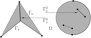
Figure 1. A particular example of $\Gamma_{s}$ (solid lines) and $\Gamma_{\nu}$ (dashed lines). Black dots represent branch points (black dots within big gray disk are branch point $f$ that lie on other sheets of the Riemann surface than the one we fixed). The white area on the figure represents domain $\Omega$.

Next, observe that

(6.19) $$\Gamma_{s}^{2}\cap\overline{\Omega}=\varnothing{\color[rgb]{1,0,0}.}$$

Indeed, since $\partial\Omega\subset\Gamma_{s}\cup\Gamma_{\nu}$ and $\Gamma_{s}^{2}$, $\Gamma^{1}_{s}\cup\Gamma_{\nu}$ are disjoint compact sets, a connected component of $\partial\Omega$ that meets $\Gamma_{s}^{2}$ is contained in it. If $z\in\Gamma_{s}^{2}\cap\partial\Omega$ lies on $\gamma_{j}^{s}$, then by analyticity of the latter each sufficiently small disk $D_{z}$ centered at $z$ is cut out by $\gamma_{j}^{s}\cap D_{z}$ into two connected components included in $D_{\nu}\cap D_{s}$, and of necessity one of them is contained in $\Omega$. Hence $\gamma_{j}^{s}\cap D_{z}$ is contained in $\partial\Omega$, and in turn so does the entire arc $\gamma_{j}^{s}$ by connectedness. Hence every component of $\Gamma_{s}^{2}\cap\partial\Omega$ consists of a union of arcs $\gamma_{j}^{s}$ connecting at their endpoints. Because $\Gamma_{s}^{2}$ has no loop, one of them has an endpoint $z_{1}\in E_{0}^{s}\cup E_{1}^{s}$ belonging to no other arc. If $z_{1}\in E_{0}^{s}$, reasoning as we did to prove (6.18) leads to the absurd conclusion that $f_{s}$ has zero jump across the initial arc. If $z_{1}\in E_{1}^{s}$, anticipating the proof of Proposition 11 once again, each sufficiently small disk $D_{z_{1}}$ centered at $z_{1}$ is cut out by $\Gamma_{s}^{2}\cap D_{z_{1}}$ into curvilinear sectors included in $D_{\nu}\cap D_{s}$, and of necessity one of them is contained in $\Omega$ whence at least two adjacent arcs $\gamma_{j}^{s}$ emanating from $z_{1}$ are included in $\partial\Omega$. This contradicts the fact that $z_{1}$ belongs to exactly one arc of the hypothesized component of $\Gamma_{s}^{2}\cap\partial\Omega$, and proves (6.19).

Finally, set

$$\Gamma_{s}^{3}:=\left[\Gamma_{s}^{1}\setminus\left(\partial\Omega\setminus E_{1}^{s}\right)\right]\cap D_{\nu}\quad\mbox{and}\quad\Gamma_{s}^{4}:=\left[\Gamma_{s}^{1}\cap\bigcup\gamma_{j}^{s}\right]\cap\partial\Omega\cap D_{\nu}.$$

Clearly

(6.20) $$\left(\Gamma_{s}^{3}\setminus E_{1}^{s}\right)\cap\overline{\Omega}=\varnothing.$$

Moreover, observing that any two arcs $\gamma_{j}^{s}$, $\gamma_{k}^{\nu}$ either coincide or meet in a (possibly empty) discrete set and arguing as we did to prove (6.19), we see that $\left[\Gamma_{s}^{1}\cap\bigcup\gamma_{j}^{s}\right]\cap\partial\Omega$ consists of subarcs of arcs $\gamma_{j}^{s}$ whose endpoints either belong to some intersection $\gamma_{j}^{s}\cap\gamma_{k}^{\nu}$ (in which case they contain this endpoint) or else lie in $E_{0}^{s}\cup E_{1}^{s}$ (in which case they do not contain this endpoint). Thus $\Gamma_{s}^{4}$ is comprised of open analytic arcs $\widetilde{\gamma}_{\ell}^{s}$ contained in $\partial\Omega\cap\bigcup\gamma_{j}^{s}$ and disjoint from $\Gamma_{\nu}$. Hence for any $z\in\Gamma_{s}^{4}$, say $z\in\widetilde{\gamma}_{\ell}^{s}$, and any disk $D_{z}$ centered at $z$ of small enough radius it holds that $D_{z}\cap\partial\Omega=D_{z}\cap\widetilde{\gamma}_{\ell}^{s}$ and that $D_{z}\setminus\widetilde{\gamma}_{\ell}^{s}$ has exactly two connected components:

(6.21) $$D_{z}\cap\Omega\neq\varnothing\quad\mbox{and}\quad D_{z}\cap\left(\overline{\mathbb{C}}\setminus\overline{\Omega}\right)\neq\varnothing$$

for if $z\in\widetilde{\gamma}_{\ell}^{s}$ was such that $D_{z}\setminus\widetilde{\gamma}_{\ell}^{s}\subset\Omega$, the jump of $f_{s}$ across $\widetilde{\gamma}_{\ell}^{s}$ would be zero as the jump of $f_{\nu}$ is zero there and $f_{s}=f_{\nu}$ in $\Omega$ (see Figure 1).

As usual, denote by $\widetilde{\nu}^{*}$ the balayage of $\nu^{*}$ onto $\mathbb{T}_{\rho}$ with $\rho\in(r,1)$ but large enough so that $\Gamma_{s}$ and $\Gamma_{\nu}$ are contained in the interior of $\mathbb{D}_{\rho}$ (see Lemma 18 for the definition of $r$). Then, according to (7.24) and (7.39), it holds that

(6.22) $$I_{\nu}[\Gamma_{s}]-I_{\nu}[\Gamma_{\nu}]=I_{D_{s}}[\widetilde{\nu}^{*}]-I_{D_{\nu}}[\widetilde{\nu}^{*}]=\mathscr{D}_{D_{s}}(V_{s})-\mathscr{D}_{D_{\nu}}(V_{\nu}),$$

where $V_{s}:=V_{D_{s}}^{\widetilde{\nu}^{*}}$ and $V_{\nu}:=V_{D_{\nu}}^{\widetilde{\nu}^{*}}$. Indeed, as $\widetilde{\nu}^{*}$ has finite energy (see Section 7.2.3), the Dirichlet integrals of $V_{s}$ and $V_{\nu}$ in the considered domains (see Section 7.4) are well-defined by Proposition 11, which is proven later but independently of the results in this section.

Set $D:=D_{\nu}\setminus(\Gamma_{s}^{2}\cup\Gamma_{s}^{3})$. Since $\left[\Gamma_{s}^{1}\setminus\left(\partial\Omega\setminus E_{1}^{s}\right)\right]$ consists of piecewise smooth arcs in $\Gamma_{s}^{1}$ whose endpoints either belong to this arc (if they lie in $E_{1}^{s}$), or to $E_{0}^{s}\cap\Gamma_{s}^{1}$ (hence also to $\Gamma_{\nu}$ by (6.18)), or else to some intersection $\gamma_{j}^{s}\cap\gamma_{k}^{\nu}$ (in which case they belong to $\Gamma_{\nu}$ again), we see that $D$ is an open set. As $V_{\nu}$ is harmonic across $\Gamma_{s}^{2}\cup\Gamma_{s}^{3}$ and $V_{s}$ is harmonic across $\Gamma_{\nu}\setminus\Gamma_{s}$, we get from (7.38) that

(6.23) $$\mathscr{D}_{D_{\nu}}(V_{\nu})=\mathscr{D}_{D}(V_{\nu})\quad\mbox{and}\quad\mathscr{D}_{D_{s}}(V_{s})=\mathscr{D}_{D\setminus\Gamma_{s}^{4}}(V_{s})$$

since $D_{s}\setminus\Gamma_{\nu}=D_{\nu}\setminus\Gamma_{s}=D\setminus\Gamma_{s}^{4}$, by inspection on using (6.18).

Now, recall that $\Gamma_{s}$ has no interior and $V_{s}\equiv 0$ on $\Gamma_{s}$, that is, $V_{s}$ is defined in the whole complex plane. So, we can define a function on $\mathbb{C}$ by putting

(6.24) $$\widetilde{V}:=\left\{\begin{array}[]{rl}V_{s},&\mbox{in}\quad\Omega,\vskip 3.0pt plus 1.0pt minus 1.0pt\\ -V_{s},&\mbox{otherwise}.\end{array}\right.$$

We claim that $\widetilde{V}$ is superharmonic in $D$ and harmonic in $D\setminus\mathbb{T}_{\rho}$. Indeed, it is clearly harmonic in $D\setminus(\Gamma_{s}^{4}\cup\mathbb{T}_{\rho})=(D_{s}\cap D_{\nu})\setminus\mathbb{T}_{\rho}$and superharmonic in a neighborhood of $\mathbb{T}_{\rho}\subset\Omega$ where its weak Laplacian is $-2\pi\widetilde{\nu}^{*}$ which is a negative measure. Moreover, $\Gamma_{s}^{4}$ is a collection of open analytic arcs such that $\partial V_{s}/\partial\textnormal{\bf n}^{+}=\partial V_{s}/\partial\textnormal{\bf n}^{-}$ by the symmetry of $\Gamma_{s}$, where $\textnormal{\bf n}^{\pm}$ are the two-sided normal on each subarc of $\Gamma_{s}^{4}$. The equality of the normals means that $V_{s}$ can be continued harmonically across each subarc of $\Gamma_{s}^{4}$ by $-V_{s}$. Hence, (6.21) and the definition of $\widetilde{V}$ yield that it is harmonic across $\Gamma_{s}^{4}$ thereby proving the claim. Thus, using (7.41) (applied with $D^{\prime}=\Omega$) and (7.38), we obtain

(6.25) $$\mathscr{D}_{D\setminus\Gamma_{s}^{4}}(V_{s})=\mathscr{D}_{D\setminus\Gamma_{s}^{4}}(\widetilde{V})=\mathscr{D}_{D}(\widetilde{V})$$

hence combining (6.22), (6.23), and (6.25), we see that

(6.26) $$I_{\nu}[\Gamma_{s}]-I_{\nu}[\Gamma_{\nu}]=\mathscr{D}_{D}(\widetilde{V})-\mathscr{D}_{D}(V_{\nu}).$$

By the first claim in Section 7.3, it holds that $h:=\widetilde{V}-V_{\nu}$ is harmonic in $D$. Observe that $h$ is not a constant function, for it tends to zero at each point of $\Gamma_{s}\cap\Gamma_{\nu}\subset\partial D$ whereas it tends to a strictly negative value at each point of $\Gamma_{s}\cap D_{\nu}\subset\overline{D}$ which is nonempty by (6.16). Then

(6.27) $$\mathscr{D}_{D}(\widetilde{V})=\mathscr{D}_{D}(V_{\nu})+\mathscr{D}_{D}(h)+2\mathscr{D}_{D}(V_{\nu},h).$$

Now, $V_{\nu}\equiv 0$ on $\Gamma_{\nu}$ and it is harmonic across $\Gamma_{s}^{2}\cup\Gamma_{s}^{3}$, hence

$$\frac{\partial h}{\partial\textnormal{\bf n}^{+}}+\frac{\partial h}{\partial\textnormal{\bf n}^{-}}=\frac{\partial{\widetilde{V}}}{\partial\textnormal{\bf n}^{+}}+\frac{\partial{\widetilde{V}}}{\partial\textnormal{\bf n}^{-}}\quad\mbox{on}\quad\Gamma_{s}^{2}\cup\Gamma_{s}^{3}.$$

Consequently, we get from (7.35), since $\widetilde{V}=-V_{s}$ in the neighborhood of $\Gamma_{s}^{2}\cup\Gamma_{s}^{3}$ by (6.19) and (6.20), that

(6.28) $$\mathscr{D}_{D}(V_{\nu},h)=-\int_{\Gamma_{s}^{2}\cup\Gamma_{s}^{3}}V_{\nu}\left(\frac{\partial\widetilde{V}}{\partial\textnormal{\bf n}^{+}}+\frac{\partial\widetilde{V}}{\partial\textnormal{\bf n}^{-}}\right)\frac{ds}{2\pi}=\int_{\Gamma_{s}^{2}\cup\Gamma_{s}^{3}}V_{\nu}\left(\frac{\partial V_{s}}{\partial\textnormal{\bf n}^{+}}+\frac{\partial V_{s}}{\partial\textnormal{\bf n}^{-}}\right)\frac{ds}{2\pi}\geq 0$$

because $V_{\nu}$ is nonnegative while $\partial V_{s}/\partial n^{+}$, $\partial V_{s}/\partial n^{-}$ are also nonnegative on $\Gamma_{s}^{2}\cup\Gamma_{s}^{3}$ as $V_{s}\geq 0$ vanishes there. Altogether, we obtain from (6.26), (6.27), and (6.28) that

$$I_{\nu}[\Gamma_{s}]-I_{\nu}[\Gamma_{\nu}]\geq\mathscr{D}_{D}(h)>0$$

by (7.40) and since $h=\tilde{V}-V_{\nu}$ is a non-constant harmonic function in $D$. This shows (6.17) and finishes the proof of the lemma. ∎

6.2. Proof of Proposition 11

It is well known that $H_{\omega,\Gamma}$ is holomorphic in the domain of harmonicity of $V_{\overline{\mathbb{C}}\setminus\Gamma}^{\omega}$, that is, in $\overline{\mathbb{C}}\setminus(\Gamma\cup\textnormal{supp}(\omega))$. It is also clear that $H_{\omega,\Gamma}^{\pm}$ exist smoothly on each $\gamma_{j}$ since $V_{\overline{\mathbb{C}}\setminus\Gamma}^{\omega}$ can be harmonically continued across each side of $\gamma_{j}$.

Denote by $\textnormal{\bf n}_{t}^{\pm}$ the one-sided unit normals at $t\in\bigcup\gamma_{j}$ and by $\tau_{t}$ the unit tangent pointing in the positive direction. Let further $n^{\pm}(t)$ be the unimodular complex numbers corresponding to vectors $\textnormal{\bf n}^{\pm}_{t}$. Then the complex number corresponding to $\tau_{t}$ is $\mp in^{\pm}(t)$ and it can be readily verified that

$$\frac{\partial V_{\overline{\mathbb{C}}\setminus\Gamma}^{\omega}}{\partial\textnormal{\bf n}^{\pm}_{t}}=2\textnormal{Re}\left(n^{\pm}(t)H_{\omega,\Gamma}^{\pm}(t)\right)\quad\mbox{and}\quad\frac{\partial\left(V_{\overline{\mathbb{C}}\setminus\Gamma}^{\omega}\right)^{\pm}}{\partial\tau_{t}}=\mp 2\textnormal{Im}\left(n^{\pm}(t)H_{\omega,\Gamma}^{\pm}(t)\right).$$

As $\left(V_{\overline{\mathbb{C}}\setminus\Gamma}^{\omega}\right)^{\pm}\equiv 0$ on $\Gamma$, the tangential derivatives above are identically zero, therefore $n^{\pm}H_{\omega,\Gamma}^{\pm}$ is real on $\Gamma$. Moreover since $n^{+}=-n^{-}$ and by the symmetry property (4.3), it holds that $H_{\omega,\Gamma}^{+}=-H_{\omega,\Gamma}^{-}$ on $\bigcup\gamma_{j}$. Hence, $H_{\omega,\Gamma}^{2}$ is holomorphic in $\overline{\mathbb{C}}\setminus(E_{0}\cup E_{1}\cup\textnormal{supp}(\omega))$. Since $E_{0}\cup E_{1}$ consists of isolated points around which $H_{\omega,\Gamma}^{2}$ is holomorphic each $e\in E_{0}\cup E_{1}$ is either a pole, a removable singularity, or an essential one. As $H_{\omega,\Gamma}$ is holomorphic on a two-sheeted Riemann surface above the point, it cannot have an essential singularity since its primitive has bounded real part $\pm V_{\overline{\mathbb{C}}\setminus\Gamma}^{\omega}$. Now, by repeating the arguments in [43, Sec. 8.2], we deduce that $(z-e)^{j_{e}-2}H^{2}_{\omega,\Gamma}(z)$ is holomorphic and non-vanishing in some neighborhood of $e$ where $j_{e}$ is the number of arcs $\gamma_{j}$ having $e$ as an endpoint, that the tangents at $e$ to these arcs exist, and that they are equiangular if $j_{e}>1$.

6.3. Proof of Theorem 14

The following theorem [25, Thm. 3] and its proof are essential in establishing Theorem 14. Before stating this result, we remind the reader that a polynomial $v$ is said to by spherically normalized if it has the form

(6.29) $$v(z)=\prod_{v(e)=0,~{}|e|\leq 1}(z-e)\prod_{v(e)=0,~{}|e|>1}(1-z/e).$$

We also recall from [25] the notions of a tame set and a tame point of a set. A point $z$ belonging to a compact set $\Gamma$ is called tame, if there is a disk centered at $z$ whose intersection with $\Gamma$ is an analytic arc. A compact set $\Gamma$ is called tame, if $\Gamma$ is non-polar and quasi-every point of $\Gamma$ is tame.

A tame compact set $\Gamma$ is said to have the S-property in the field $\psi$, assumed to be harmonic in some neighborhood of $\Gamma$, if $\textnormal{supp}(\omega_{\Gamma,\psi})$ forms a tame set as well, every tame point of $\textnormal{supp}(\omega_{\Gamma,\psi})$ is also a tame point of $\Gamma$, and the equality in (4.4) holds at each tame point of $\textnormal{supp}(\omega_{\Gamma,\psi})$.

Whenever the tame compact set $\Gamma$ has connected complement in a simply connected region $G\supset\Gamma$ and $g$ is holomorphic in $G\setminus\Gamma$, we write $\oint_{\Gamma}g(t)\,dt$ for the contour integral of $g$ over some (hence any) system of curves encompassing $\Gamma$ once in $G$ in the positive direction. Likewise, the Cauchy integral $\oint_{\Gamma}g(t)/(z-t)\,dt$ can be defined at any $z\in\overline{\mathbb{C}}\setminus\Gamma$ by choosing the previous system of curves in such a way that it separates $z$ from $\Gamma$.

If $g$ has limits from each side at tame points of $\Gamma$, and if these limits are integrable with respect to linear measure on $\Gamma$, then the previous integrals may well be rewritten as integrals on $\Gamma$ with $g$ replaced by its jump across $\Gamma$. However, this is not what is meant by the notation $\oint_{\Gamma}$.

Theorem GR.

Let $G\subset\mathbb{D}$ be a simply connected domain and $\Gamma\subset G$ be a tame compact set with connected complement. Let also $g$ be holomorphic in $G\setminus\Gamma$ and have continuous limits on $\Gamma$ from each side in the neighborhood of every tame point, whose jump across $\Gamma$ is non-vanishing q.e. Further, let $\{\Psi_{n}\}$ be a sequence of functions that satisfy:

1. $\Psi_{n}$ is holomorphic in $G$ and $-\frac{1}{2n}\log|\Psi_{n}|\to\psi$ locally uniformly there, where $\psi$ is harmonic in $G$;

2. $\Gamma$ possesses the S-property in the field $\psi$ (see (4.4)).

Then, if the polynomials $q_{n}$, $\deg(q_{n})\leq n$, satisfy the orthogonality relations

(6.30) $$\oint_{\Gamma}q_{n}(t)l_{n-1}(t)\Psi_{n}(t)g(t)dt=0,\quad\mbox{for any}\quad l_{n-1}\in\mathcal{P}_{n-1},$$

then $\mu_{n}\stackrel{{\scriptstyle*}}{{\to}}\omega_{\Gamma,\psi}$, where $\mu_{n}$ is the normalized counting measure of zeros of $q_{n}$. Moreover, if the polynomials $q_{n}$ are spherically normalized, it holds that

(6.31) $$\left|A_{n}(z)\right|^{1/2n}\stackrel{{\scriptstyle\scriptsize\textnormal{cap}}}{{\rightarrow}}\exp\{-c(\psi;\Gamma)\}\quad\mbox{in}\quad\overline{\mathbb{C}}\setminus\Gamma,$$

where $c(\psi;\Gamma)$ is the modified Robin constant (Section 7.1.2), and

(6.32) $$A_{n}(z):=\oint_{\Gamma}q_{n}^{2}(t)\frac{(\Psi_{n}g)(t)dt}{z-t}=\frac{q_{n}(z)}{l_{n}(z)}\oint_{\Gamma}(l_{n}q_{n})(t)\frac{(\Psi_{n}g)(t)dt}{z-t},$$

where $l_{n}$ can be any nonzero polynomial of degree at most $n$.

Proof of Theorem 14.

Let $E_{n}$ be the sets constituting the interpolation scheme $\mathcal{E}$. Set $\Psi_{n}$ to be the reciprocal of the spherically normalized polynomial with zeros at the finite elements of $E_{n}$, i.e., $\Psi_{n}=1/\tilde{v}_{n}$, where $\tilde{v}_{n}$ is the spherical renormalization of $v_{n}$ (see Definition 13 and (6.29)). Then the functions $\Psi_{n}$ are holomorphic and non-vanishing in $\mathbb{C}\setminus\textnormal{supp}(\mathcal{E})$ (in particular, in $\mathbb{D}$), $\frac{1}{2n}\log|\Psi_{n}|\stackrel{{\scriptstyle\scriptsize\textnormal{cap}}}{{\rightarrow}}U^{\nu}$ in $\overline{\mathbb{C}}\setminus\textnormal{supp}(\nu^{*})$ by Lemma 21, and this convergence is locally uniform in $\mathbb{D}$ by definition of the asymptotic distribution and since $\log 1/|z-t|$ is continuous on a neighborhood of $\textnormal{supp}(\mathcal{E})$ for fixed $z\in\mathbb{D}$. As $U^{\nu}$ is harmonic in $\mathbb{D}$, requirement (1) of Theorem GR is fulfilled with $G=\mathbb{D}$ and $\psi=-U^{\nu}$. Further, it follows from Theorem 12 that $\Gamma_{\nu}$ is a symmetric set. In particular it is a smooth cut, hence it is tame with tame points $\cup_{j}\gamma_{j}$. Moreover, since $\Gamma_{\nu}$ is regular, we have that $\textnormal{supp}(\omega_{\Gamma,\psi})=\Gamma_{\nu}$ by (7.18) and properties of balayage (Section 7.2.2). Thus, by the remark after Definition 10, symmetry implies that $\Gamma_{\nu}$ possesses the S-property in the field $-U^{\nu}$ and therefore requirement (2) of Theorem GR is also fulfilled. Let now $Q$, $\deg(Q)=:m$, be a fixed polynomial such that the only singularities of $Qf$ in $\mathbb{D}$ belong to $E_{f}$. Then $Qf$ is holomorphic and single-valued in $\mathbb{D}\setminus\Gamma_{\nu}$, it extends continuously from each side on $\cup\gamma_{j}$, and has a jump there which is continuous and non-vanishing except possibly at countably many points. All the requirement of Theorem GR are then fulfilled with $g=Qf$.

Let $L\subset\mathbb{D}$ be a smooth Jordan curve that separates $\Gamma_{\nu}$ and the poles of $f$ (if any) from $\mathcal{E}$. Denote by $q_{n}$ the spherically normalized denominators of the multipoint Padé approximants to $f$ associated with $\mathcal{E}$. It is a standard consequence of Definition 13 (see e.g. [25, sec. 1.5.1]) that

(6.33) $$\int_{L}z^{j}q_{n}(z)\Psi_{n}(z)f(z)dz=0,\quad j\in\{0,\ldots,n-1\}.$$

Clearly, relations (6.33) imply that

(6.34) $$\oint_{\Gamma_{\nu}}(lq_{n}\Psi_{n}fQ)(t)dt=0,\quad\deg(l)<n-m.$$

Equations (6.34) differ from (6.30) only in the reduction of the degree of polynomials $l$ by a constant $m$. However, to derive the first conclusion of Theorem GR, namely that $\mu_{n}\stackrel{{\scriptstyle*}}{{\to}}\omega_{\Gamma,\psi}$, orthogonality relations (6.30) are used solely when applied to a specially constructed sequence $\{l_{n}\}$ such that $l_{n}=l_{n,1}l_{n,2}$, where $\deg(l_{n,1})\leq n\theta$, $\theta<1$, and $\deg(l_{n,2})=o(n)$ as $n\to\infty$ (see the proof of [25, Thm. 3] in between equations (27) and (28)). Thus, the proof is still applicable in our situation, to the effect that the normalized counting measures of the zeros of $q_{n}$ converge weak^∗ to $\widehat{\nu}^{*}=\omega_{\Gamma_{\nu},-U^{\nu}}$, see (7.23).

For each $n\in\mathbb{N}$, let $q_{n,m}$, $\deg(q_{n,m})=n-m$, be a divisor of $q_{n}$. Observe that the polynomials $q_{n,m}$ have exactly the same asymptotic zero distribution in the weak^∗ sense as the polynomials $q_{n}$. Put

(6.35) $$A_{n,m}(z):=\oint(q_{n,m}q_{n})(t)\frac{(\Psi_{n}fQ)(t)dt}{z-t},\quad z\in D_{\nu}.$$

Due to orthogonality relations (6.34), $A_{n,m}$ can be equivalently rewritten as

(6.36) $$A_{n,m}(z):=\frac{q_{n,m}(z)}{l_{n-m}(z)}\oint(l_{n-m}q_{n})(t)\frac{(\Psi_{n}fQ)(t)dt}{z-t},\quad z\in D_{\nu},$$

where $l_{n-m}$ is an arbitrary polynomial of degree at most $n-m$. Formulae (6.35) and (6.36) differ from (6.32) in the same manner as orthogonality relations (6.34) differ from those in (6.30). Examination of the proof of [25, Thm. 3] (see the discussion there between equations (33) and (37)) shows that limit (6.31) is proved using expression (6.32) for $A_{n}$ with a choice of polynomials $l_{n}$ that satisfy some set of asymptotic requirements and can be chosen to have the degree $n-m$. Hence it still holds that

(6.37) $$|A_{n,m}(z)|^{1/2n}\stackrel{{\scriptstyle\scriptsize\textnormal{cap}}}{{\rightarrow}}\exp\left\{-c(-U^{\nu};\Gamma_{\nu})\right\}\quad\mbox{in}\quad D_{\nu}.$$

Finally, using the Hermite interpolation formula like in [52, Lem. 6.1.2], the error of approximation has the following representation

(6.38) $$(f-\Pi_{n})(z)=\frac{A_{n,m}(z)}{(q_{n,m}q_{n}Q\Psi_{n})(z)},\quad z\in D_{\nu}.$$

From Lemma 21 we know that $\log(1/|q_{n}|)/n\stackrel{{\scriptstyle\scriptsize\textnormal{cap}}}{{\rightarrow}}V_{*}^{\widehat{\nu^{*}}}=V^{\widehat{\nu^{*}}}$ in $D_{\nu}$, since ordinary and spherically normalized potentials coincide for measures supported in $\overline{\mathbb{D}}$. This fact together with (6.37) and (6.38) easily yield that

$$|f-\Pi_{n}|^{1/2n}\stackrel{{\scriptstyle\scriptsize\textnormal{cap}}}{{\rightarrow}}\exp\left\{-c(-U^{\nu};\Gamma_{\nu})+V^{\widehat{\nu}^{*}}-U^{\nu}\right\}\quad\mbox{in}\quad D_{\nu}\setminus\textnormal{supp}(\nu^{*}).$$

Therefore, (5.1) follows from (7.20) and the fact that $U^{\nu}=V_{*}^{\nu^{*}}$ by the remark at the beginning of Section 7.2.4. ∎

6.4. Proof of Theorem 4, Theorem 7, Corollary 8, Theorem 6, and Theorem 5

Proof of Theorem 4.

Let $\Gamma\in\mathcal{K}_{f}(G)$ be a smooth cut for $f$ that satisfies (2.5) and $\Theta$ be a conformal map of $\mathbb{D}$ onto $G$. Set $K:=\Theta^{-1}(\Gamma)$. Then we get from the conformal invariance of the condenser capacity (see (7.7)) and the maximum principle for harmonic functions that

$$\textnormal{cap}(\Gamma,T)=\textnormal{cap}(K,\mathbb{T})\quad\mbox{and}\quad V_{\overline{\mathbb{C}}\setminus K}^{\omega_{(K,\mathbb{T})}}=V_{\overline{\mathbb{C}}\setminus\Gamma}^{\omega_{(\Gamma,T)}}\circ\Theta\quad\mbox{in}\quad\mathbb{D}.$$

As $\Theta$ is conformal in $\mathbb{D}$, it can be readily verified that $V_{\overline{\mathbb{C}}\setminus K}^{\omega_{(K,\mathbb{T})}}$ satisfies (2.5) as well (naturally, on $K$). Univalence of $\Theta$ also implies that the continuation properties of $(f\circ\Theta)(\Theta^{\prime})^{1/2}$ in $\mathbb{D}$ are exactly the same as those of $f$ in $G$. Moreover, this is also true for $f_{\Theta}$, the orthogonal projection of $(f\circ\Theta)(\Theta^{\prime})^{1/2}$ from $L^{2}$ onto $\bar{H}_{0}^{2}$ (see Section 3). Indeed, $f_{\Theta}$ is holomorphic in $\mathbb{O}$ by its very definition and can be continued analytically across $\mathbb{T}$ by $(f\circ\Theta)(\Theta^{\prime})^{1/2}$ minus the orthogonal projection of the latter from $L^{2}$ onto $H^{2}$, which is holomorphic in $\mathbb{D}$ by definition. Thus, $f_{\Theta}\in\mathcal{A}(\mathbb{D})$ and $\Gamma\in\mathcal{K}_{f}(G)$ if and only if $K\in\mathcal{K}_{f_{\Theta}}$. Therefore, it is enough to consider only the case $G=\mathbb{D}$.

Let $\Gamma\in\mathcal{K}_{f}$ be a smooth cut for $f$ that satisfies (2.5) and K be the set of minimal condenser capacity (cf. Theorem Theorem S). We must prove that $\Gamma=\textnormal{K}$. Set, for brevity, $D_{\Gamma}:=\overline{\mathbb{C}}\setminus\Gamma$, $V_{\Gamma}:=V_{D_{\Gamma}}^{\omega_{(\mathbb{T},\Gamma)}}$, $D_{\textnormal{K}}:=\overline{\mathbb{C}}\setminus\textnormal{K}$, $V_{\textnormal{K}}:=V_{D_{\textnormal{K}}}^{\omega_{(\mathbb{T},\textnormal{K})}}$, and $\Omega$ to be the unbounded component of $D_{\textnormal{K}}\cap D_{\Gamma}$. Let also $f_{D_{\Gamma}}$ and $f_{D_{\textnormal{K}}}$ indicate the meromorphic branches of $f$ in $D_{\Gamma}$ and $D_{\textnormal{K}}$, respectively. Arguing as we did to prove (6.19), we see that no connected component of $\partial\Omega$ can lie entirely in $\Gamma\setminus\textnormal{K}$ (resp. $\textnormal{K}\setminus\Gamma$) otherwise the jump of $f_{D_{\Gamma}}$ (resp. $f_{D_{\textnormal{K}}}$) across some subarc of $\Gamma$ (resp. K) would vanish. Hence by connectedness

(6.39) $$\Gamma\cap\textnormal{K}\cap\partial\Omega\neq\varnothing.$$

First, we deal with the special situation where $\omega_{(\mathbb{T},\textnormal{K})}=\omega_{(\mathbb{T},\Gamma)}$. Then $V_{\Gamma}-V_{\textnormal{K}}$ is harmonic in $\Omega$ by the first claim in Section 7.3. As both potentials are constant in $\mathbb{O}\subset\Omega$, we get that $V_{\Gamma}=V_{\textnormal{K}}+\textnormal{const.}$ in $\Omega$. Since K and $\Gamma$ are regular sets, potentials $V_{\Gamma}$ and $V_{\textnormal{K}}$ extend continuously to $\partial\Omega$ and vanish at $\partial\Omega\cap\Gamma\cap\textnormal{K}$ which is non-empty by (6.39). Thus, equality of the equilibrium measures means that $V_{\Gamma}\equiv V_{\textnormal{K}}$ in $\overline{\Omega}$. However, because $V_{\Gamma}$ (resp. $V_{\textnormal{K}}$) vanishes precisely on $\Gamma$ (resp. K), this is possible only if $\partial\Omega\subset\Gamma\cap\textnormal{K}$. Taking complements in $\overline{\mathbb{C}}$, we conclude that $D_{\Gamma}\cup D_{\textnormal{K}}$, which is connected and contains $\infty$, does not meet $\partial\Omega$. Therefore $D_{\Gamma}\cup D_{\textnormal{K}}\subset\Omega\subset D_{\Gamma}\cap D_{\textnormal{K}}$, hence $D_{\Gamma}=D_{\textnormal{K}}$ thus $\Gamma=\textnormal{K}$, as desired.

In the rest of the proof we assume for a contradiction that $\Gamma\neq\textnormal{K}$. Then $\omega_{(\mathbb{T},\textnormal{K})}\neq\omega_{(\mathbb{T},\Gamma)}$ in view of what precedes, and therefore

(6.40) $$\mathscr{D}_{D_{\textnormal{K}}}(V_{\textnormal{K}})=I_{D_{\textnormal{K}}}\left[\omega_{(\mathbb{T},\textnormal{K})}\right]<I_{D_{K}}\left[\omega_{(\mathbb{T},\Gamma)}\right]=\mathscr{D}_{D_{\textnormal{K}}}(V_{D_{\textnormal{K}}}^{\omega_{(\mathbb{T},\Gamma)}})$$

by (7.39) and since the Green equilibrium measure is the unique minimizer of the Green energy.

The argument now follows the lines of the proof of Lemma 20. Namely, we write

$$\Gamma=E_{0}^{\Gamma}\cup E_{1}^{\Gamma}\cup\bigcup\gamma_{j}^{\Gamma},\qquad\textnormal{K}=E_{0}^{\textnormal{K}}\cup E_{1}^{\textnormal{K}}\cup\bigcup\gamma_{j}^{\textnormal{K}},$$

and we define the sets $\Gamma^{1}$, $\Gamma^{2}$, $\Gamma^{3}$, $\Gamma^{4}$ like we did in that proof for $\Gamma^{1}_{s}$, $\Gamma_{s}^{2}$, $\Gamma_{s}^{3}$, $\Gamma_{s}^{4}$, upon replacing $D_{s}$ by $D_{\Gamma}$, $D_{\nu}$ by $D_{\textnormal{K}}$, $E_{j}^{s}$ by $E_{j}^{\Gamma}$, $E_{j}^{\nu}$ by $E_{j}^{\textnormal{K}}$, $\gamma_{j}^{s}$ by $\gamma_{j}^{\Gamma}$ and $\gamma_{j}^{\nu}$ by $\gamma_{j}^{\textnormal{K}}$. The same reasoning that led to us to (6.19) and (6.20) yields

(6.41) $$\Gamma^{2}\cap\overline{\Omega}=\varnothing,\qquad\left(\Gamma^{3}\setminus E_{1}^{\Gamma}\right)\cap\overline{\Omega}=\varnothing.$$

Subsequently we set $D:=D_{\textnormal{K}}\setminus(\Gamma^{2}\cup\Gamma^{3})$ and we prove in the same way that it is an open set satisfying

(6.42) $$\mathscr{D}_{D_{K}}(V_{D_{\textnormal{K}}}^{\omega_{(\mathbb{T},\Gamma)}})=\mathscr{D}_{D}(V_{D_{\textnormal{K}}}^{\omega_{(\mathbb{T},\Gamma)}})\quad\mbox{and}\quad\mathscr{D}_{D_{\Gamma}}(V_{\Gamma})=\mathscr{D}_{D\setminus\Gamma^{4}}(V_{\Gamma})$$

(compare (6.23)). Defining $\widetilde{V}$ as in (6.24) with $V_{s}$ replaced by $V_{\Gamma}$, and using the symmetry of $\Gamma$ (that is, (2.5) with $\Gamma$ instead of K, which allows us to continue $V_{\Gamma}$ harmonically by $-V_{\Gamma}$ across each arc $\gamma_{j}^{\Gamma}$) we find that $\widetilde{V}$ is harmonic in $D\setminus\mathbb{T}$, superharmonic in $D$, and that

(6.43) $$\mathscr{D}_{D_{\Gamma}\setminus\Gamma^{4}}(V_{\Gamma})=\mathscr{D}_{D}(\widetilde{V})$$

(compare (6.25)). Next, we set $h:=\widetilde{V}-V_{D_{\textnormal{K}}}^{\omega_{(\mathbb{T},\Gamma)}}$ which is harmonic in $D$ by the first claim in Section 7.3, and since $h=V_{\Gamma}-V_{D_{\textnormal{K}}}^{\omega_{(\Gamma,\mathbb{T})}}$ in $\Omega\supset\mathbb{T}$. Because $\widetilde{V}=-V_{\Gamma}$ in the neighborhood of $\Gamma_{s}^{2}\cup\Gamma_{s}^{3}$ by (6.41), the same computation as in (6.28) gives us

$$\mathscr{D}_{D}(V_{D_{\textnormal{K}}}^{\omega_{(\mathbb{T},\Gamma)}},h)\geq 0,$$

so we get from (7.39), (6.42), (6.43), (7.40) and (6.40) that

(6.44) $$I_{D_{\Gamma}}[\omega_{(\mathbb{T},\Gamma)}] = \mathscr{D}_{D_{\Gamma}}(V_{\Gamma})=\mathscr{D}_{D}(\widetilde{V})=\mathscr{D}_{D}(V_{D_{\textnormal{K}}}^{\omega_{(\mathbb{T},\Gamma)}}+h)$$

$$= \mathscr{D}_{D}(V_{D_{\textnormal{K}}}^{\omega_{(\mathbb{T},\Gamma)}})+2\mathscr{D}_{D}(V_{D_{\textnormal{K}}}^{\omega_{(\mathbb{T},\Gamma)}},h)+\mathscr{D}_{D}(h)$$

$$\geq \mathscr{D}_{D_{\textnormal{K}}}(V_{D_{\textnormal{K}}}^{\omega_{(\mathbb{T},\Gamma)}})+\mathscr{D}_{D}(h)>\mathscr{D}_{D_{\textnormal{K}}}(V_{\textnormal{K}})=I_{D_{\textnormal{K}}}[\omega_{(\mathbb{T},\textnormal{K})}].$$

However, it holds that

$$I_{D_{\textnormal{K}}}[\omega_{(\mathbb{T},\textnormal{K})}]=1/\textnormal{cap}(\textnormal{K},\mathbb{T})\quad\mbox{and}\quad I_{D_{\Gamma}}[\omega_{(\mathbb{T},\Gamma)}]=1/\textnormal{cap}(\Gamma,\mathbb{T})$$

by (7.6). Thus, (6.44) yields that $\textnormal{cap}(\Gamma,\mathbb{T})<\textnormal{cap}(\textnormal{K},\mathbb{T})$, which is impossible by the very definition of K. This contradiction finishes the proof. ∎

Proof of Theorem 7.

Let $\{r_{n}\}$ be a sequence of irreducible critical points for $f$. Further, let $\nu_{n}$ be the normalized counting measures of the poles of $r_{n}$ and $\nu$ be a weak^∗ limit point of $\{\nu_{n}\}$, i.e., $\nu_{n}\stackrel{{\scriptstyle*}}{{\to}}\nu$, $n\in\mathbb{N}_{1}\subset\mathbb{N}$. Recall that all the poles of $r_{n}$ are contained in $\mathbb{D}$ and therefore $\textnormal{supp}(\nu)\subseteq\overline{\mathbb{D}}$.

By Theorem 12, there uniquely exists a minimal set $\Gamma_{\nu}$ for Problem $(f,\nu)$. Let $Z_{n}$ be the set of poles of $r_{n}$, where each pole appears with twice its multiplicity. As mentioned in Section 3, each $r_{n}$ interpolates $f$ at the points of $Z_{n}^{*}$, counting multiplicity. Hence, $\{r_{n}\}_{n\in\mathbb{N}_{1}}$ is the sequence of multipoint Padé approximants associated with the triangular scheme $\mathcal{E}=\{Z_{n}^{*}\}_{n\in\mathbb{N}_{1}}$ that has asymptotic distribution $\nu^{*}$, where $\nu^{*}$ is the reflection of $\nu$ across $\mathbb{T}$. So, according to Theorem 14 (applied for subsequences), it holds that $\nu=\widehat{\nu}^{*}$, $\textnormal{supp}(\nu)=\Gamma_{\nu}$, i.e., $\nu$ is the balayage of its own reflection across $\mathbb{T}$ relative to $D_{\nu}$.

Applying Lemma 25, we deduce that $\nu$ is the Green equilibrium distribution on $\Gamma_{\nu}$ relative to $\mathbb{D}$, that is, $\nu=\omega_{(\Gamma_{\nu},\mathbb{T})}$, and $\widetilde{\nu}$, the balayage of $\nu$ onto $\mathbb{T}$, is the Green equilibrium distribution on $\mathbb{T}$ relative to $D_{\nu}$, that is, $\widetilde{\nu}=\omega_{(\mathbb{T},\Gamma_{\nu})}$. Moreover, Lemma 25 yields that $V_{D_{\nu}}^{\nu^{*}}=V_{D_{\nu}}^{\widetilde{\nu}}$ in $\mathbb{D}$ and therefore $V_{D_{\nu}}^{\widetilde{\nu}}$ enjoys symmetry property (2.5) by Theorem 12. Hence, we get from Theorem 4 that $\Gamma_{\nu}=\textnormal{K}$, the set of minimal condenser capacity for $f$, and that $\nu=\omega_{(\textnormal{K},\mathbb{T})}$. Since $\nu$ was an arbitrary limit point of $\{\nu_{n}\}$, we have that $\nu_{n}\stackrel{{\scriptstyle*}}{{\to}}\omega_{(\textnormal{K},\mathbb{T})}$ as $n\to\infty$. Finally, observe that (3.2) is a direct consequence of Theorem 14.

To prove (3.3), we need to go back to representation (6.38), where $q_{n}\in\mathcal{M}_{n}$ is the denominator of an irreducible critical point $r_{n}$ and $q_{n,m}$, $\deg(q_{n,m})=n-m$, is an arbitrary divisor of $q_{n}$, while $\Psi_{n}=1/\widetilde{q}_{n}^{2}$ with $\widetilde{q}_{n}(z)=z^{n}\overline{q_{n}(1/\bar{z})}$.

Denote by $b_{n}$ the Blaschke product $q_{n}/\widetilde{q}_{n}$. It is easy to check that $b_{n}(z)\overline{b_{n}(1/\bar{z})}\equiv 1$ by algebraic properties of Blaschke products. Thus, (6.38) yields that

(6.45) $$(f-r_{n})(z)=\overline{b^{2}_{n}(1/\bar{z})}(l_{n,m}A_{n,m}/Q)(z),\quad z\in\overline{\mathbb{O}}.$$

where $l_{n,m}$ is the polynomial of degree $m$ such that $q_{n}=q_{n,m}l_{n,m}$. Choose $\epsilon>0$ so small that $\textnormal{K}\subset\mathbb{D}_{1-\epsilon}$ (see Theorem 12). As $l_{n,m}$ is an arbitrary divisor of $q_{n}$ of degree $m$, we can choose it to have zeros only in $\mathbb{D}_{1-\epsilon}$ for all $n$ large enough (this is possible since in full proportion the zeros of $q_{n}$ approach K). Then it holds that

(6.46) $$\lim_{n\to\infty}|l_{n,m}/Q|^{1/2n}=1$$

uniformly on $\overline{\mathbb{O}}$. Further, by (3.2) and the last claim of Lemma 25, we have that

(6.47) $$|f-r_{n}|^{1/2n}\stackrel{{\scriptstyle\scriptsize\textnormal{cap}}}{{\rightarrow}}\exp\left\{-\frac{1}{\textnormal{cap}(\textnormal{K},\mathbb{T})}\right\}\quad\mbox{on}\quad\mathbb{T}.$$

As any Blaschke product is unimodular on the unit circle, we deduce from (6.45)–(6.47) with the help of (6.37) (i.e., $A_{n,m}$ goes to a constant) that

$$|A_{n,m}|^{1/2n}\stackrel{{\scriptstyle\scriptsize\textnormal{cap}}}{{\rightarrow}}\exp\left\{-\frac{1}{\textnormal{cap}(\textnormal{K},\mathbb{T})}\right\}\quad\mbox{in}\quad\overline{\mathbb{C}}\setminus\textnormal{K}.$$

Then we get from Lemma 22 that

(6.48) $$\limsup_{n\to\infty}|A_{nm}|^{1/2n}\leq\exp\left\{-\frac{1}{\textnormal{cap}(\textnormal{K},\mathbb{T})}\right\}$$

uniformly on closed subsets of $\overline{\mathbb{C}}\setminus\textnormal{K}$, in particular, uniformly on $\overline{\mathbb{O}}$. Set $q_{n,\epsilon}$ for the monic polynomial whose zeros are those of $q_{n}$ lying in $\mathbb{D}_{1-\epsilon}$. Put $n_{\epsilon}:=\deg(q_{n,\epsilon})$, $\widetilde{q}_{n,\epsilon}(z)=z^{n_{\epsilon}}\overline{q_{n,\epsilon}(1/\bar{z})}$, and let $\nu_{n,\epsilon}$ be the normalized counting measure of the zeros of $q_{n,\epsilon}$. As $\nu_{n}\stackrel{{\scriptstyle*}}{{\to}}\omega_{(\textnormal{K},\mathbb{T})}$, it is easy to see that $n_{\epsilon}/n\to 1$ and that $\nu_{n,\epsilon}\stackrel{{\scriptstyle*}}{{\to}}\omega_{(\textnormal{K},\mathbb{T})}$ when $n\to+\infty$. Thus, by the principle of descent (Section 7.2.5), it holds that

(6.49) $$\limsup_{n\to\infty}|q_{n,\epsilon}|^{1/n}=\limsup_{n\to\infty}|q_{n,\epsilon}|^{1/{n_{\epsilon}}}\leq\exp\left\{-V^{\omega_{(\textnormal{K},\mathbb{T})}}\right\},$$

locally uniformly in $\mathbb{C}$. In another connection, since $\log|1-z\bar{u}|$ is continuous for $(z,u)\in\mathbb{D}_{1/(1-\epsilon)}\times\mathbb{D}_{1-\epsilon}$, it follows easily from the weak^∗ convergence of $\nu_{n,\epsilon}$ that

(6.50) $$\lim_{n\to\infty}|\widetilde{q}_{n,\epsilon}(z)|^{1/n}=\lim_{n\to\infty}|\widetilde{q}_{n,\epsilon}(z)|^{1/{n_{\epsilon}}}=\exp\left\{\int\log|1-z\bar{u}|d\omega_{(\textnormal{K},\mathbb{T})}(u)\right\},$$

uniformly in $\overline{\mathbb{D}}$. Put $b_{n,\epsilon}:=q_{n,\epsilon}/\widetilde{q}_{n.\epsilon}$. Since the Green function of $\mathbb{D}$ with pole at $u$ is given by $\log|(1-z\bar{u})/(z-u)|$, we deduce from (6.49), (6.50), and a simple majorization that

$$\limsup_{n\to\infty}|b_{n}|^{1/n}\leq\limsup_{n\to\infty}|b_{n,\epsilon}|^{1/n}\leq\exp\left\{-V_{\mathbb{D}}^{\omega_{(\textnormal{K},\mathbb{T})}}\right\}$$

uniformly in $\overline{\mathbb{D}}$. Besides, the Green function of $\mathbb{O}$ is still given by $\log|(1-z\bar{u})/(z-u)|$, hence $V_{\mathbb{D}}^{\omega}(1/\bar{z})=V_{\mathbb{O}}^{\omega^{*}}(z)$, $z\in\mathbb{O}$, where $\omega$ is any measure supported in $\mathbb{D}$. Thus, we derive that

(6.51) $$\limsup_{n\to\infty}|b_{n}^{2}(1/\bar{z})|^{1/2n}\leq\exp\left\{-V_{\mathbb{O}}^{\omega_{(\textnormal{K},\mathbb{T})}^{*}}(z)\right\}$$

holds uniformly on $\overline{\mathbb{O}}$. Combining (6.45)–(6.51), we deduce that

$$\limsup_{n\to\infty}|f-r_{n}|^{1/2n}\leq\exp\left\{-\frac{1}{\textnormal{cap}(\textnormal{K},\mathbb{T})}-V_{\mathbb{O}}^{\omega_{(\textnormal{K},\mathbb{T})}^{*}}\right\}$$

uniformly on $\overline{\mathbb{O}}$. This finishes the proof of the theorem since $V_{\overline{\mathbb{C}}\setminus\textnormal{K}}^{\omega_{(\textnormal{K},\mathbb{T})}^{*}}=\frac{1}{\textnormal{cap}(\textnormal{K},\mathbb{T})}+V_{\mathbb{O}}^{\omega_{(\textnormal{K},\mathbb{T})}^{*}}$ in $\overline{\mathbb{O}}$ by Lemma 25, the maximum principle for harmonic functions applied in $\mathbb{O}$, and the fact that the difference of two Green potentials of the same measure but on different domains is harmonic in a neighborhood of the support of that measure by the first claim in Section 7.3. ∎

Proof of Corollary 8.

It follows from (3.3) and Lemma 25 that

$$\limsup_{n\to\infty}\|f-r_{n}\|_{\mathbb{T}}^{1/2n}\leq\exp\left\{-\frac{1}{\textnormal{cap}(\textnormal{K},\mathbb{T})}\right\}.$$

On the other hand, by (3.2) and the very definition of convergence in capacity, we have for any $\epsilon>0$ small enough that

$$|f-r_{n}|>\left(\exp\left\{-\frac{1}{\textnormal{cap}(\textnormal{K},\mathbb{T})}\right\}-\epsilon\right)^{2n}\quad\mbox{on}\quad\mathbb{T}\setminus S_{n,\epsilon},$$

where $\textnormal{cap}(S_{n,\epsilon})\to 0$ as $n\to\infty$. In particular, it means that $|S_{n,\epsilon}|\to 0$ by [45, Thm. 5.3.2(d)], where $|S_{n,\epsilon}|$ is the arclength measure of $S_{n,\epsilon}$. Hence, we have that

$$\liminf_{n\to\infty}\|f-r_{n}\|_{2}^{1/2n} \geq \lim_{n\to\infty}\left(\frac{|\mathbb{T}\setminus S_{n,\epsilon}|}{2\pi}\right)^{1/4n}\left(\exp\left\{-\frac{1}{\textnormal{cap}(\textnormal{K},\mathbb{T})}\right\}-\epsilon\right)$$

$$= \exp\left\{-\frac{1}{\textnormal{cap}(\textnormal{K},\mathbb{T})}\right\}-\epsilon.$$

As $\epsilon$ was arbitrary and since $\|f-r_{n}\|_{2}\leq 2\pi\|f-r_{n}\|_{\mathbb{T}}$, this finishes the proof of the corollary. ∎

Proof of Theorem 6.

Let $\Theta$ be the conformal map of $\mathbb{D}$ onto $G$. Observe that $\Theta^{\prime}$ is a holomorphic function in $\mathbb{D}$ with integrable trace on $\mathbb{T}$ since $T$ is rectifiable [20, Thm. 3.12], and that $\Theta$ extends in a continuous manner to $\mathbb{T}$ where it is absolutely continuous. Hence, $(f\circ\Theta)(\Theta^{\prime})^{1/2}\in L^{2}$. Moreover, $g$ lies in $E_{n}^{2}(G)$ if and only if $(g\circ\Theta)(\Theta^{\prime})^{1/2}$ lies in $H_{n}^{2}:=H^{2}\mathcal{M}^{-1}_{n}$. Indeed, denote by $E^{\infty}(G)$ the space of bounded holomorphic functions in $G$ and set $E_{n}^{\infty}(G):=E^{\infty}(G)\mathcal{M}^{-1}_{n}(G)$. It is clear that $g\in E_{n}^{\infty}(G)$ if and only if it is meromorphic in $G$ and bounded outside a compact subset thereof. This makes it obvious that $g\in E_{n}^{\infty}(G)$ if and only if $g\circ\Theta\in H_{n}^{\infty}:=H^{\infty}\mathcal{M}^{-1}_{n}$, where $H^{\infty}$ is the space of bounded holomorphic functions in $\mathbb{D}$. It is also easy to see that $E_{n}^{2}(G)=E^{2}(G)E_{n}^{\infty}(G)$. Since it is known that $g\in E^{2}(G)$ if and only if $(g\circ\Theta)(\Theta^{\prime})^{1/2}\in H^{2}$ [20, corollary to Thm. 10.1], the claim follows. Notice also that $g_{n}$ is a best approximant for $f$ from $E_{n}^{2}(G)$ if and only if $(g_{n}\circ\Theta)(\Theta^{\prime})^{1/2}$ is a best approximant for $(f\circ\Theta)(\Theta^{\prime})^{1/2}$ from $H_{n}^{2}$. This is immediate from the change of variable formula, namely,

$$\|f-g\|_{2,T}^{2}=\int_{\mathbb{T}}|f\circ\Theta-g\circ\Theta|^{2}|\Theta^{\prime}|d\theta=\|(f\circ\Theta)(\Theta^{\prime})^{1/2}-(g_{n}\circ\Theta)(\Theta^{\prime})^{1/2}\|_{2}^{2},$$

where we used the fact that $|d\Theta(e^{i\theta})|=|\Theta^{\prime}(e^{i\theta})|d\theta$ a.e. on $\mathbb{T}$ [20, Thm. 3.11].

Now, let $g_{n}$ be a best meromorphic approximants for $f$ from $E^{2}_{n}(G)$. As $L^{2}=H^{2}\oplus\bar{H}^{2}_{0}$, it holds that $(g_{n}\circ\Theta)(\Theta^{\prime})^{1/2}=g_{n}^{+}+r_{n}$ and $(f\circ\Theta)(\Theta^{\prime})^{1/2}=f^{+}+f^{-}$, where $g_{n}^{+},f^{+}\in H^{2}$ and $r_{n},f^{-}\in\bar{H}^{2}_{0}$. Moreover, it can be easily checked that $r_{n}\in\mathcal{R}_{n}$ and, as explained at the beginning of the proof of Theorem 4, that $f^{-}\in\mathcal{A}(\mathbb{D})$. Since by Parseval’s relation

$$\|(f\circ\Theta)(\Theta^{\prime})^{1/2}-(g_{n}\circ\Theta)(\Theta^{\prime})^{1/2}\|_{2}^{2}=\|f^{+}-g_{n}^{+}\|_{2}^{2}+\|f^{-}-r_{n}\|_{2}^{2},$$

we immediately deduce that $g_{n}^{+}=f^{+}$ and that $r_{n}$ is an $\bar{H}^{2}_{0}$-best rational approximant for $f^{-}$. Moreover, by the conformal invariance of the condenser capacity (see (7.7)), $\textnormal{cap}(\textnormal{K},T)=\textnormal{cap}(\Theta^{-1}(\textnormal{K}),\mathbb{T})$. It is also easy to verify that $K\in\mathcal{K}_{f}(G)$ if and only if $\Theta^{-1}(K)\in\mathcal{K}_{f^{-}}(\mathbb{D})$. Hence, we deduce from Theorem 7 and the remark thereafter that

$$|f^{-}-r_{n}|^{1/2n}\stackrel{{\scriptstyle\scriptsize\textnormal{cap}}}{{\rightarrow}}\exp\left\{V_{\mathbb{D}}^{\omega_{(\Theta^{-1}(\textnormal{K}),\mathbb{T})}}-\frac{1}{\textnormal{cap}(\Theta^{-1}(\textnormal{K}),\mathbb{T})}\right\}\quad\mbox{in}\quad\mathbb{D}\setminus\Theta^{-1}(\textnormal{K}).$$

The result then follows from the conformal invariance of the Green equilibrium measures, Green capacity, and Green potentials and the fact that, since $\Theta$ is locally Lipschitz-continuous in $\mathbb{D}$, it cannot locally increase the capacity by more than a multiplicative constant [45, Thm. 5.3.1]. ∎

Proof of Theorem 5.

By Theorem S and decomposition (7.16), the set K of minimal condenser capacity for $f$ is a smooth cut, hence a tame compact set with tame points $\cup\gamma_{j}$, such that

$$\frac{\partial}{\partial\textnormal{\bf n}^{+}}V^{\widehat{\omega}_{(T,\textnormal{K})}-\omega_{(T,\textnormal{K})}}=\frac{\partial}{\partial\textnormal{\bf n}^{-}}V^{\widehat{\omega}_{(T,\textnormal{K})}-\omega_{(T,\textnormal{K})}}\quad\mbox{on}\quad\bigcup\gamma_{j},$$

where $\widehat{\omega}_{(T,\textnormal{K})}$ is the balayage of $\omega_{(T,\textnormal{K})}$ onto K. As $\widehat{\omega}_{(T,\textnormal{K})}$ is the weighted equilibrium distribution on K in the field $V^{-\omega_{(T,\textnormal{K})}}$ (see (7.18)), the set K possesses the S-property in the sense of (4.4). If $f$ is holomorphic in $\overline{\mathbb{C}}\setminus\textnormal{K}$ and since it extends continuously from both sides on each $\gamma_{j}$ with a jump that can vanish in at most countably many points, we get from [25, Thm. 1^′] that

(6.52) $$\lim_{n\to\infty}\rho_{n,\infty}^{1/2n}(f,T)=\exp\left\{-\frac{1}{\textnormal{cap}(\textnormal{K},T)}\right\}.$$

However, Theorem 1^′ in [25] is obtained as an application of Theorem GR. Since the latter also holds for functions in $\mathcal{A}(G)$, that is, those that are meromorphic in $\overline{\mathbb{C}}\setminus\textnormal{K}$, (see the explanation in the proof of Theorem 14), (6.52) is valid for these functions as well. As $\rho_{n,2}(f,T)\leq|T|\rho_{n,\infty}(f,T)$, where $|T|$ is the arclength of $T$, we get from (6.52) that

$$\limsup_{n\to\infty}\rho_{n,2}^{1/2n}(f,T)\leq\exp\left\{-\frac{1}{\textnormal{cap}(\textnormal{K},T)}\right\}.$$

On the other hand, let $g_{n}$ be a best meromorphic approximants for $f$ from $E_{n}^{2}(G)$ as in Theorem 6. Using the same notation, it was shown that $((f-g_{n})\circ\Theta)(\Theta^{\prime})^{1/2}=(f^{-}-r_{n})$, where $r_{n}$ is a best $\bar{H}_{0}^{2}$-rational approximant for $f^{-}$ from $\mathcal{R}_{n}$. Hence, we deduce from the chain of equalities

$$\|f-g_{n}\|_{2,T}=\|(f\circ\Theta)(\Theta^{\prime})^{1/2}-(g_{n}\circ\Theta)(\Theta^{\prime})^{1/2}\|_{2}=\|f^{-}-r_{n}\|_{2}$$

and Corollary 8 that

$$\lim_{n\to\infty}\|f-g_{n}\|_{2,T}^{1/2n}=\exp\left\{-\frac{1}{\textnormal{cap}(\Theta^{-1}(\textnormal{K}),\mathbb{T})}\right\}=\exp\left\{-\frac{1}{\textnormal{cap}(\textnormal{K},T)}\right\}.$$

As $\rho_{n,2}(f,T)\geq\|f-g_{n}\|_{2,T}$ by the very definition of $g_{n}$ and the inclusion $\mathcal{R}_{n}(G)\subset E^{2}_{n}(G)$, the lower bound for the limit inferior of $\rho_{n,2}^{1/2n}(f,T)$ follows. ∎

7. Some Potential Theory

Below we give a brief account of logarithmic potential theory that was used extensively throughout the paper. We refer the reader to the monographs [45, 47] for a thorough treatment.

7.1. Capacities

In this section we introduce, logarithmic, weighted, and condenser capacities.

7.1.1. Logarithmic Capacity

The logarithmic potential of a finite positive measure $\omega$, compactly supported in $\mathbb{C}$, is defined by

$$V^{\omega}(z):=-\int\log|z-u|d\omega(u),\quad z\in\mathbb{C}.$$

The function $V^{\omega}$ is superharmonic with values in $(-\infty,+\infty]$ and is not identically $+\infty$. The logarithmic energy of $\omega$ is defined by

$$I[\omega]:=\int V^{\omega}(z)d\omega(z)=-\iint\log|z-u|d\omega(u)d\omega(z).$$

As $V^{\omega}$ is bounded below on $\textnormal{supp}(\omega)$, it follows that $I[\omega]\in(-\infty,+\infty]$.

Let $F\subset\mathbb{C}$ be compact and $\Lambda(F)$ denote the set of all probability measures supported on $F$. If the logarithmic energy of every measure in $\Lambda(F)$ is infinite, we say that $F$ is polar. Otherwise, there exists a unique $\omega_{F}\in\Lambda(F)$ that minimizes the logarithmic energy over all measures in $\Lambda(F)$. This measure is called the equilibrium distribution on $F$ and it is known that $\omega_{F}$ is supported on the outer boundary of $F$, i.e., the boundary of the unbounded component of the complement of $F$. Hence, if $K$ and $F$ are two compact sets with identical outer boundaries, then $\omega_{K}=\omega_{F}$.

The logarithmic capacity, or simply the capacity, of $F$ is defined as

$$\textnormal{cap}(F)=\exp\{-I[\omega_{F}]\}.$$

By definition, the capacity of an arbitrary subset of $\mathbb{C}$ is the supremum of the capacities of its compact subsets. We agree that the capacity of a polar set is zero. It follows readily from what precedes that the capacity of a compact set is equal to the capacity of its outer boundary.

We say that a property holds quasi everywhere (q.e.) if it holds everywhere except on a set of zero capacity. We also say that a sequence of functions $\{h_{n}\}$ converges in capacity to a function $h$, $h_{n}\stackrel{{\scriptstyle\scriptsize\textnormal{cap}}}{{\rightarrow}}h$, on a compact set $K$ if for any $\epsilon>0$ it holds that

$$\lim_{n\to\infty}\textnormal{cap}\left(\left\{z\in K:~{}|h_{n}(z)-h(z)|\geq\epsilon\right\}\right)=0.$$

Moreover, we say that the sequence $\{h_{n}\}$ converges in capacity to $h$ in a domain $D$ if it converges in capacity on each compact subset of $D$. In the case of an unbounded domain, $h_{n}\stackrel{{\scriptstyle\scriptsize\textnormal{cap}}}{{\rightarrow}}h$ around infinity if $h_{n}(1/\cdot)\stackrel{{\scriptstyle\scriptsize\textnormal{cap}}}{{\rightarrow}}h(1/\cdot)$ around the origin.

When the support of $\omega$ is unbounded, it is easier to consider $V_{*}^{\omega}$, the spherical logarithmic potential of $\omega$, i.e.,

(7.1) $$V_{*}^{\omega}(z)=\int k(z,u)d\omega(u),\quad k(z,u)=-\left\{\begin{array}[]{ll}\log|z-u|,&\mbox{if}~{}|u|\leq 1,\vskip 3.0pt plus 1.0pt minus 1.0pt\\ \log|1-z/u|,&\mbox{if}~{}|u|>1.\end{array}\right.$$

The advantages of dealing with the spherical logarithmic potential shall become apparent later in this section.

7.1.2. Weighted Capacity

Let $F$ be a non-polar compact set and $\psi$ be a lower semi-continuous function on $F$ such that $\psi<\infty$ on a non-polar subset of $F$. For any measure $\omega\in\Lambda(F)$, we define the weighted energy of $\omega$ by

$$I_{\psi}[\omega]:=I[\omega]+2\int\psi d\omega.$$

Then there exists a unique measure $\omega_{F,\psi}$, the weighted equilibrium distribution on $F$, that minimizes $I_{\psi}[\omega]$ among all measures in $\Lambda(F)$ [47, Thm. I.1.3]. Clearly, $\omega_{F,\psi}=\omega_{F}$ when $\psi\equiv 0$.

The measure $\omega_{F,\psi}$ admits the following characterization [47, Thm. I.3.3]. Let $\omega$ be a positive Borel measure with compact support and finite energy such that $V^{\omega}+\psi$ is constant q.e. on $\textnormal{supp}(\omega)$ and at least as large as this constant q.e. on $F$. Then $\omega=\omega_{F,\psi}$. The value of $V^{\omega}+\psi$ q.e. on $\textnormal{supp}(\omega_{F,\psi})$ is called the modified Robin constant and it can be expressed as

(7.2) $$c(\psi;F)=I_{\psi}[\omega_{F,\psi}]-\int\psi d\omega_{F,\psi}=I[\omega_{F,\psi}]+\int\psi d\omega_{F,\psi}.$$

The weighted capacity of $F$ is defined as $\displaystyle\textnormal{cap}_{\psi}(F)=\exp\left\{-I_{\psi}[\omega_{F,\psi}]\right\}$.

7.1.3. Condenser Capacity

Let now $D$ be a domain with non-polar boundary and $g_{D}(\cdot,u)$ be the Green function for $D$ with pole at $u\in D$. That is, the unique function such that

• $g_{D}(z,u)$ is a positive harmonic function in $D\setminus\{u\}$, which is bounded outside each neighborhood of $u$;

• $\displaystyle g_{D}(z,u)+\left\{\begin{array}[]{ll}-\log|z|,&\mbox{if}\quad u=\infty,\\ \log|z-u|,&\mbox{if}\quad u\neq\infty,\end{array}\right.$ is bounded near $u$;

• $\displaystyle\lim_{z\to\xi,\;z\in D}g_{D}(z,u)=0$ for quasi every $\xi\in\partial D$.

For definiteness, we set $g_{D}(z,u)=0$ for any $z\in\overline{\mathbb{C}}\setminus\overline{D}$, $u\in D$. Thus, $g_{D}(z,u)$ is defined throughout the whole extended complex plane.

It is known that $g_{D}(z,u)=g_{D}(u,z)$, $z,u\in D$, and that the subset of $\partial D$ for which (iii) holds does not depend on $u$. Points of continuity of $g_{D}(\cdot,u)$ on $\partial D$ are called regular, other points on $\partial D$ are called irregular; the latter form $F_{\sigma}$ polar set (in particular, it is totally disconnected). When $F$ is compact and non-polar, we define regular points of $F$ as points of continuity of $g_{D}(\cdot,\infty)$, where $D$ is the unbounded component of the complement of $F$. In particular, all the inner points of $F$ are regular, i.e., the irregular points of $F$ are contained in the outer boundary of $F$, that is, $\partial D$. We call $F$ regular if all the point of $F$ are regular.

It is useful to notice that for a compact non-polar set $F$ the uniqueness of the Green function implies that

(7.3) $$g_{\overline{\mathbb{C}}\setminus F}(z,\infty)\equiv-\log\textnormal{cap}(F)-V^{\omega_{F}}(z),\quad z\in\overline{\mathbb{C}}\setminus F,$$

by property (ii) in the definition of the Green function and the characterization of the equilibrium potential (see explanation before (7.2)).

In analogy to the logarithmic case, one can define the Green potential and the Green energy of a positive measure $\omega$ supported in a domain $D$ as

$$V_{D}^{\omega}(z):=\int g_{D}(z,u)d\omega(u)\quad\mbox{and}\quad I_{D}[\omega]:=\iint g_{D}(z,w)d\omega(z)d\omega(w).$$

Exactly as in the logarithmic case, if $E$ is a non-polar compact subset of $D$, there exists a unique measure $\omega_{(E,\partial D)}\in\Lambda(E)$ that minimizes the Green energy among all measures in $\Lambda(E)$. This measure is called the Green equilibrium distribution on $E$ relative to $D$. The condenser capacity of $E$ relative to $D$ is defined as

$$\textnormal{cap}(E,\partial D):=1/I_{D}[\omega_{(E,\partial D)}].$$

It is known that the Green potential of the Green equilibrium distribution satisfies

(7.4) $$V_{D}^{\omega_{(E,\partial D)}}(z)=\frac{1}{\textnormal{cap}(E,\partial D)},\quad\mbox{for q.e.}\quad z\in E.$$

Moreover, the equality in (7.4) holds at all the regular points of $E$. Furthermore, it is known that $\omega_{(E,\partial D)}$ is supported on the outer boundary of $E$. That is,

(7.5) $$\omega_{(E,\partial D)}=\omega_{(\partial\Omega,\partial D)},$$

where $\Omega$ is the unbounded component of the complement of $E$.

Let $F$ be a non-polar compact set, $D$ any component of the complement of $F$, and $E$ a non-polar subset of $D$. Then we define $\omega_{(E,F)}$ and $\textnormal{cap}(E,F)$ as $\omega_{(E,\partial D)}$ and $\textnormal{cap}(E,\partial D)$, respectively. It is known that

(7.6) $$\textnormal{cap}(E,F)=\textnormal{cap}(F,E),$$

where $F$ and $E$ are two disjoint compact sets with connected complements. That is, the condenser capacity is symmetric with respect to its entries and only the outer boundary of a compact plays a role in calculating the condenser capacity.

As in the logarithmic case, the Green equilibrium measure can be characterized by the properties of its potential. Namely, if $\omega$ has finite Green energy, $\textnormal{supp}(\omega)\subseteq E$, $V_{D}^{\omega}$ is constant q.e. on $\textnormal{supp}(\omega)$ and is at least as large as this constant q.e. on $E$, then $\omega=\omega_{(E,\partial D)}$ [47, Thm. II.5.12]. Using this characterization and the conformal invariance of the Green function, one can see that the condenser capacity is also conformally invariant. In other words, it holds that

(7.7) $$\textnormal{cap}(E,\partial D)=\textnormal{cap}(\phi(E),\partial\phi(D)),$$

where $\phi$ is a conformal map of $D$ onto its image.

7.2. Balayage

In this section we introduce the notion of balayage of a measure and describe some of its properties.

7.2.1. Harmonic Measure

Let $D$ be a domain with compact boundary $\partial D$ of positive capacity and $\{\omega_{z}\}_{z\in D}$, be the harmonic measure for $D$. That is, $\{\omega_{z}\}_{z\in D}$ is the collection of probability Borel measures on $\partial D$ such that for any bounded Borel function $f$ on $\partial D$ the function

$$P_{D}f(z):=\int fd\omega_{z},\quad z\in D,$$

is harmonic [45, Thm. 4.3.3] and $\lim_{z\to x}P_{D}f(z)=f(x)$ for any regular point $x\in\partial D$ at which $f$ is continuous [45, Thm. 4.1.5].

The generalized minimum principle [47, Thm. I.2.4] says that if $u$ is superharmonic, bounded below, and $\liminf_{z\to x,z\in D}u(z)\geq m$ for q.e. $x\in\partial D$, then $u>m$ in $D$ unless $u$ is a constant. This immediately, implies that

(7.8) $$P_{D}h=h$$

for any $h$ which is bounded and harmonic in $D$ and extends continuously to q.e. point of $\partial D$.

For $z\in\mathbb{C}$ and $z\neq w\in D\setminus\{\infty\}$, set

(7.9) $$h_{D}(z,w):=\left\{\begin{array}[]{l}\log|z-w|+g_{D}(z,w),\quad\mbox{if}~{}D~{}\mbox{is bounded},\vskip 3.0pt plus 1.0pt minus 1.0pt\\ \log|z-w|+g_{D}(z,w)-g_{D}(z,\infty)-g_{D}(w,\infty),\quad\mbox{otherwise}.\end{array}\right.$$

Observe that by the properties of Green function $h_{D}(z,\cdot)$ is harmonic at $z$. Moreover, it can be computed using (7.3) that $\lim_{|zw|\to\infty}h_{D}(z,w)=\log\textnormal{cap}(\partial D)$ when $D$ is unbounded. Therefore, $h_{D}(z,w)$ is defined for all $w\in D$ and $z\in\mathbb{C}\cup D$. Moreover, for each $w\in D$, the function $h_{D}(\cdot,w)$ is bounded and harmonic in $D$ and extends continuously to every regular point of $\partial D$. It is also easy to see that $h_{D}(z,w)=h_{D}(w,z)$ for $z,w\in D$. Hence, we deduce from (7.8) that

(7.10) $$h_{D}(z,w)=\left\{\begin{array}[]{l}P_{D}(\log|z-\cdot|)(w),\quad\mbox{if}~{}D~{}\mbox{is bounded},\vskip 3.0pt plus 1.0pt minus 1.0pt\\ P_{D}(\log|z-\cdot|-g(z,\infty))(w),\quad\mbox{otherwise},\end{array}\right.$$

$z\in(\mathbb{C}\cup D)\setminus\partial D$, for $w\in D$ and all regular $w\in\partial D$.

7.2.2. Balayage

Let $\nu$ be a finite Borel measure supported in $D$. The balayage of $\nu$, denoted by $\widehat{\nu}$, is a Borel measure on $\partial D$ defined by

(7.11) $$\widehat{\nu}(B):=\int\omega_{t}(B)d\nu(t)$$

for any Borel set $B\subset\partial D$. Since $\omega_{z}(\partial D)=1$, the total mass of $\widehat{\nu}$ is equal to the total mass of $\nu$. Moreover, it follows immediately from (7.11) that $\widehat{\delta}_{z}=\omega_{z}$, $z\in D$. In particular, if $D$ is unbounded, $\widehat{\delta}_{\infty}=\omega_{\infty}=\omega_{\partial D}$ (for the last equality see [45, Thm. 4.3.14]). In other words, $\widehat{\delta}_{\infty}$ is the logarithmic equilibrium distribution on $\partial D$.

It is a straightforward consequence of (7.11) that

(7.12) $$\int fd\widehat{\nu}=\int P_{D}fd\nu$$

for any bounded Borel function on $\partial D$. Thus, we can conclude from (7.8) and (7.12) that

(7.13) $$\int hd\widehat{\nu}=\int hd\nu$$

for any function $h$ which is bounded and harmonic in $D$ and extends continuously to q.e. point of $\partial D$.

Assume now that $x\in\partial D$ is a regular point and $W$ an open neighborhood of $x$ in $\partial D$. Let further $f\geq 0$ be a continuous function on $\partial D$ which is supported in $W$ and such that $f(x)>0$. Since $P_{D}f(z)\to f(x)$ when $D\ni z\to x$, we see from (7.12) that $\hat{\nu}(W)>0$. In particular, $\partial D\setminus\textnormal{supp}(\hat{\nu})$ is polar.

Let $D^{\prime}$ be a domain with non-polar compact boundary such that $\overline{D}\subset D^{\prime}$ and let $\{\omega_{z}^{\prime}\}_{z\in D^{\prime}}$ be the harmonic measure for $D^{\prime}$. For any Borel set $B\subset\partial D^{\prime}$ it holds that $\omega_{z}^{\prime}(B)$ is a harmonic function in $D$ with continuous boundary values on $\partial D$. Thus,

$$\int\omega_{z}^{\prime}(B)d\widehat{\nu}(z)=\int\omega_{z}^{\prime}(B)d\nu(z)$$

by (7.13). This immediately implies that

(7.14) $$\widetilde{\nu}=\widetilde{\widehat{\nu}},$$

where $\widetilde{\nu}$ is the balayage of $\nu$ onto $\partial D^{\prime}$. In other words, balayage can be done step by step.

7.2.3. Balayage and Potentials

It readily follows from (7.9), (7.10), and (7.13) that

(7.15) $$\int h_{D}(z,w)d\nu(w)=\left\{\begin{array}[]{l}-V^{\widehat{\nu}}(z),\quad\mbox{if}~{}D~{}\mbox{is bounded},\vskip 3.0pt plus 1.0pt minus 1.0pt\\ -V^{\widehat{\nu}}(z)-g_{D}(z,\infty),\quad\mbox{otherwise},\end{array}\right.\quad z\in(\mathbb{C}\cup D)\setminus\partial D.$$

Clearly, the left-hand side of (7.15) extends continuously to q.e. $z\in\partial D$. Thus, the same is true for the right-hand side. In particular, this means that $V^{\widehat{\nu}}$ is bounded on $\partial D$ and continuous q.e. on $\partial D$. Hence, $\widehat{\nu}$ has finite energy.

In the case when $\nu$ is compactly supported in $D$, formula (7.15) has even more useful consequences. Namely, it holds that

(7.16) $$V_{D}^{\nu}(z)=V^{\nu-\widehat{\nu}}(z)+c(\nu;D),\quad z\in\overline{\mathbb{C}},$$

where $c(\nu;D)=\int g_{D}(z,\infty)d\nu(z)$ if $D$ is unbounded and $c(\nu;D)=0$ otherwise, and where we used a continuity argument to extend (7.16) to every $z\in\overline{\mathbb{C}}$. This, in turn, yields that

(7.17) $$V^{\widehat{\nu}}(z)=V^{\nu}(z)+c(\nu;D)\quad\mbox{for q.e.}\quad z\in\mathbb{C}\setminus D,$$

where equality holds for all $z\in\mathbb{C}\setminus\overline{D}$ and also at all regular points of $\partial D$. Moreover, employing the characterization of weighted equilibrium measures, we obtain from (7.17) that

(7.18) $$\widehat{\nu}=\omega_{\partial D,-V^{\nu}}\quad\mbox{and}\quad c(-V^{\nu};\partial D)=c(\nu;D).$$

If a measure $\nu$ is not compactly supported, the logarithmic potential of $\nu$ may not be defined. However, representations similar to (7.16)–(7.18) can be obtained using the spherical logarithmic potentials. Indeed, it follows from (7.15) that

$$(V_{*}^{\nu}-V^{\widehat{\nu}}-V_{D}^{\nu})(z) = \int\left[k(z,u)+\log|z-u|-g_{D}(u,\infty)\right]d\nu(u)$$

$$= \int_{|u|>1}\left[\log|u|-g_{D}(u,\infty)\right]d\nu(u)-\int_{|u|\leq 1}g_{D}(u,\infty)d\nu(u).$$

As the right-hand side of the chain of the equalities above is a finite constant and $V_{D}^{\nu}$ vanishes quasi everywhere on $\partial D$, we deduce as in (7.16)–(7.18) that this constant is $-c(-V_{*}^{\nu};\partial D)$ and that

(7.19) $$\widehat{\nu}=\omega_{\partial D,-V_{*}^{\nu}}.$$

Moreover, it holds that

(7.20) $$V_{D}^{\nu}(z)=V_{*}^{\nu}(z)-V^{\widehat{\nu}}(z)+c(-V_{*}^{\nu};\partial D),\quad z\in\overline{\mathbb{C}}.$$

Let now $D$ be a bounded domain and $K$ be a compact non-polar subset of $D$. If $E\subseteq K$ is also non-polar and compact, then

(7.21) $$|I_{D}[\omega_{E}]-I[\omega_{E}]|\leq\max_{z\in K,u\in\partial D}|\log|z-u||$$

by integrating both sides of (7.16) against $\omega_{E}$ with $\nu=\omega_{E}$. This, in particular, yields that

(7.22) $$\left|\frac{1}{\textnormal{cap}(E,\partial D)}+\log\textnormal{cap}(E)\right|\leq\max_{z\in K,u\in\partial D}|\log|z-u||.$$

7.2.4. Weighted Capacity in the Field $-U^{\nu}$

Let $\nu$ be a probability Borel measure supported in $\overline{\mathbb{D}}$, $K\subset\mathbb{D}_{r}$, $r<1$, be a compact non-polar set, and $D$ be the unbounded component of the complement of $K$. Further, let $U^{\nu}(z)=-\int\log|1-z\bar{u}|d\nu(u)$ as defined in (4.1). It is immediate to see that $U^{\nu}=V_{*}^{\nu^{*}}$, where, as usual, $\nu^{*}$ is the reflection of $\nu$ across $\mathbb{T}$. In particular, it follows from (7.19), (7.20), and the characterization of the weighted equilibrium distribution that

(7.23) $$\widehat{\nu}^{*}=\omega_{K,-U^{\nu}},$$

where $\widehat{\nu}^{*}$ is the balayage of $\nu^{*}$ onto $\partial D$ relative to $D$. Thus, $\omega_{K,-U^{\nu}}$ is supported on the outer boundary of $K$ and remains the same for all sets whose outer boundaries coincide up to a polar set. In another connection, it holds that

$$U^{\nu}(z)=-\int\log|1-z/u|d\nu^{*}(u)=-\int\log|1-z/u|d\widetilde{\nu}^{*}(u)=V^{\widetilde{\nu}^{*}}(z)-V^{\widetilde{\nu}^{*}}(0)$$

for any $z\in\mathbb{D}_{r}$ by (7.13) and harmonicity of $\log|1-z/u|$ as a function of $u\in\mathbb{D}_{r}^{*}$, where $\widetilde{\nu}^{*}$ is the balayage of $\nu^{*}$ onto $\mathbb{T}_{r}$. It is also true that $\widehat{\nu}^{*}=\widehat{\widetilde{\nu^{*}}}$ by (7.14). Thus,

$$I_{\nu}[K]=I[\widehat{\nu}^{*}]-2\int V^{\widetilde{\nu}^{*}}d\widehat{\nu}^{*}+2V^{\widetilde{\nu}^{*}}(0),$$

where $I_{\nu}[K]$ was defined in (4.2). Using the harmonicity of $V^{\widehat{\nu}^{*}}+g_{D}(\cdot,\infty)$ in $D$ and continuity at regular points of $\partial D$, (7.13), the Fubini-Tonelli theorem, and (7.16), we obtain that

(7.24) $$I_{\nu}[K] = \int\left(V^{\widehat{\nu}^{*}}(z)+g_{D}(z,\infty)\right)d\widehat{\nu}^{*}(z)-2\int V^{\widehat{\nu}^{*}}d\widetilde{\nu}^{*}+2V^{\widetilde{\nu}^{*}}(0)$$

$$= \int\left(V_{D}^{\widetilde{\nu}^{*}}(z)-V^{\widetilde{\nu}^{*}}(z)-c(\widetilde{\nu}^{*};D)+g_{D}(z,\infty)\right)d\widetilde{\nu}^{*}(z)+2V^{\widetilde{\nu}^{*}}(0)$$

$$= I_{D}[\widetilde{\nu}^{*}]-I[\widetilde{\nu}^{*}]+2V^{\widetilde{\nu}^{*}}(0).$$

Equation (7.24), in particular, means that the problem of maximizing $I_{\nu}[\cdot]$ among the sets in $\mathbb{D}_{r}$ is equivalent to the problem of maximizing the Green energy of $\widetilde{\nu}^{*}$ among the domains with boundary in $\mathbb{D}_{r}$.

7.2.5. Weak^∗ Convergence and Convergence in Capacity

By a theorem of F. Riesz, the space of complex continuous functions on $\overline{\mathbb{C}}$, endowed with the sup norm, has dual the space of complex measures on $\overline{\mathbb{C}}$ normed with the mass of the total variation (the so-called strong topology for measures). We say that a sequence of Borel measures $\{\omega_{n}\}$ on $\overline{\mathbb{C}}$ converges weak^∗ to a Borel measure $\omega$ if $\int fd\omega_{n}\to\int fd\omega$ for any complex continuous function $f$ on $\overline{\mathbb{C}}$. By the Banach-Alaoglu theorem, any bounded sequence of measures has a subsequence that converges in the weak^∗ sense. Conversely, by the Banach-Steinhaus theorem, a weak^∗ converging sequence is bounded.

We shall denote weak^∗ convergence by the symbol $\stackrel{{\scriptstyle*}}{{\to}}$. Weak^∗ convergence of measures implies some convergence properties of logarithmic and spherical logarithmic potentials, which we mention below.

The following statement is known as the Principle of Descent [47, Thm. I.6.8]. Let $\{\omega_{n}\}$ be a sequence of probability measures all having support in a fixed compact set. Suppose that $\omega_{n}\stackrel{{\scriptstyle*}}{{\to}}\omega$ and $z_{n}\to z$, $z_{n},z\in\mathbb{C}$. Then

$$V^{\omega}(z)\leq\liminf_{n\to\infty}V^{\omega_{n}}(z_{n})\quad\mbox{and}\quad I[\omega]\leq\liminf_{n\to\infty}I[\omega_{n}].$$

Weak^∗ convergence of measures entails some convergence in capacity of their spherical potentials. This is stated rather informally in [25, Sec. 3 and 4], but the result is slightly subtle because, as examples show, convergence in capacity generally occurs outside the support of the limiting measure only. A precise statement is as follows.

Lemma 21.

Let $\{\omega_{n}\}$ be a sequence of positive Borel measures such that $\omega_{n}\stackrel{{\scriptstyle*}}{{\to}}\omega$. Then $V_{*}^{\omega_{n}}\stackrel{{\scriptstyle\scriptsize\textnormal{cap}}}{{\rightarrow}}V_{*}^{\omega}$ in $\overline{\mathbb{C}}\setminus\textnormal{supp}(\omega)$. In particular, if $\omega$ is the zero measure, then the spherically normalized potentials $V_{*}^{\omega_{n}}$ converge to zero in capacity in the whole extended complex plane.

Proof.

Suppose first that $\omega_{n}$ converges weak^∗ to the zero measure. Then the convergence is actually strong. Assume moreover that the measures $\omega_{n}$ are supported on a fixed compact set $K\subset\mathbb{C}$. Let $G$ be a simply connected domain that contains $K$, $L$ be a Jordan curve that contains the closure of $G$ in its interior, and $D$ be a bounded simply connected domain that contains $L$. Fix $\epsilon>0$ and define $E_{n}:=\{z\in D:~{}V_{D}^{\omega_{n}}(z)>\epsilon\}$. By superharmonicity of $V_{D}^{\omega_{n}}$ the set $E_{n}$ is open, and we can assume $E_{n}\subset G$ by taking $n$ large enough. If $E_{n}$ is empty then $\textnormal{cap}(E_{n})=0$, otherwise let $E\subset E_{n}$ be a nonpolar compact set. Then the Green equilibrium potential $V_{D}^{\omega_{(E,\partial D)}}$ is bounded above by $1/\textnormal{cap}(E,\partial D)$ [47, Thm. 5.11] which is finite. Hence $h:=V_{D}^{\omega_{n}}-\varepsilon\textnormal{cap}(E,\partial D)V_{D}^{\omega_{(E,\partial D)}}$ is superharmonic and bounded below in in $D\setminus E$, with $\liminf h(z)\geq 0$ as $z$ tends to $\partial E\cup\partial D$. By the minimum principle, we thus have

$$V_{D}^{\omega_{n}}\geq\epsilon\textnormal{cap}(E,\partial D)V_{D}^{\omega_{(E,\partial D)}}\quad\mbox{in}\quad D\setminus E.$$

Set

$$m:=\min_{u\in\overline{G}}\min_{z\in L}g_{D}(z,u)>0.$$

Clearly, $V_{D}^{\omega_{(E,\partial D)}}(z)>m$, $z\in L$, thus

$$V_{D}^{\omega_{n}}\geq\epsilon m\textnormal{cap}(E,\partial D)\quad\mbox{on}\quad L.$$

Hence, in view of (7.22) applied with $K=\overline{G}$, we get

$$-\log\textnormal{cap}(E_{n})=-\sup_{E\subset E_{n}}\log\textnormal{cap}(E)\geq\frac{\epsilon m}{\sup_{L}V_{D}^{\omega_{n}}}-C$$

where $C$ is independent of $n$. Using the uniform convergence to 0 of $V_{D}^{\omega_{n}}$ on $L$, we get that $\textnormal{cap}(E_{n})\to 0$ as $n\to\infty$, that is, $V_{D}^{\omega_{n}}\stackrel{{\scriptstyle\scriptsize\textnormal{cap}}}{{\rightarrow}}0$ in $D$. Let, as usual, $\widehat{\omega}_{n}$ be the balayage of $\omega_{n}$ onto $\partial D$. Since $|\widehat{\omega}_{n}|=|\omega_{n}|\to 0$ as $n\to\infty$, we have that $V^{\widehat{\omega}_{n}}\to 0$ locally uniformly in $D$. Combining this fact with (7.16), we get that $V^{\omega_{n}}\stackrel{{\scriptstyle\scriptsize\textnormal{cap}}}{{\rightarrow}}0$ in $D$. Let $u$ be an arbitrary point in $G$. Then $\{V^{\omega_{n}}+|\omega_{n}|\log|\cdot-u|\}$ is a sequence of harmonic functions in $\overline{\mathbb{C}}\setminus G$. It is easy to see that this sequence converges uniformly to 0 there. As $|\omega_{n}|\log|\cdot-u|\stackrel{{\scriptstyle\scriptsize\textnormal{cap}}}{{\rightarrow}}0$ in $\overline{\mathbb{C}}$, we deduce that $V^{\omega_{n}}\stackrel{{\scriptstyle\scriptsize\textnormal{cap}}}{{\rightarrow}}0$ in the whole extended complex plane and so does $V_{*}^{\omega_{n}}=V^{\omega_{n}}+\int\log^{+}|u|d\omega_{n}$ (cf. (7.1)) since $\textnormal{supp}(\omega_{n})\subset K$.

Next, let $\{\omega_{n}\}$ be an arbitrary sequence of positive measures that converges to the zero measure. As the restriction ${\omega_{n}}_{|{\overline{\mathbb{D}}}}$ converges to zero, we may assume by the first part of the proof that $\textnormal{supp}(\omega_{n})\subset\overline{\mathbb{O}}$. It can be easily seen from the definition of the spherical potential (7.1) that

(7.25) $$V_{*}^{\omega_{n}}(1/z)=V_{*}^{\tilde{\omega}_{n}}(z)+|\omega_{n}|\log|z|,\quad z\in\mathbb{C}\setminus\{0\},$$

where $\tilde{\omega}_{n}$ is the reciprocal measure of $\omega_{n}$, i.e., $\tilde{\omega}_{n}(B)=\omega_{n}(\{z:1/z\in B\})$ for any Borel set $B$. Clearly $\tilde{\omega}_{n}\to 0$ and $\textnormal{supp}(\tilde{\omega}_{n})\subset\overline{\mathbb{D}}$, thus from the first part of the proof we get $V_{*}^{\tilde{\omega}_{n}}\stackrel{{\scriptstyle\scriptsize\textnormal{cap}}}{{\rightarrow}}0$. Since $|\omega_{n}|\to 0$, we also see by inspection that $|\omega_{n}|\log|z|\stackrel{{\scriptstyle\scriptsize\textnormal{cap}}}{{\rightarrow}}0$. Therefore, by (7.25), we obtain that $V_{*}^{\omega_{n}}(1/z)\stackrel{{\scriptstyle\scriptsize\textnormal{cap}}}{{\rightarrow}}0$ which is equivalent to $V_{*}^{\omega_{n}}\stackrel{{\scriptstyle\scriptsize\textnormal{cap}}}{{\rightarrow}}0$.

Let now $\{\omega_{n}\}$ be a sequence of positive measures converging weak^∗ to some Borel measure $\omega\neq 0$. If $\textnormal{supp}(\omega)=\overline{\mathbb{C}}$, there is nothing to prove. Otherwise, to each $\varepsilon>0$, we set $F_{\varepsilon}:=\{z\in\overline{\mathbb{C}}:~{}d_{c}(z,\textnormal{supp}(\omega))\geq\varepsilon\}$ where $d_{c}$ is the chordal distance on the Riemann sphere. Pick a continuous function $f$, with $0\leq f\leq 1$, which is identically $1$ on $F_{\varepsilon}$ and supported in $F_{\varepsilon/2}$.By the positivity of $\omega_{n}$ and its weak^∗ convergence to $\omega$, we get

$$0\leq\lim_{n\to+\infty}\omega_{n}(F_{\varepsilon})\leq\lim_{n\to+\infty}\int f\,d\omega_{n}=\int f\,d\omega=0.$$

From this, it follows easily that if $\varepsilon_{n}\to 0$ slowly enough, then the restriction $\omega_{n}^{1}:={\omega_{n}}_{|F_{\varepsilon_{n}}}$ converges strongly to the zero measure. Therefore $V_{*}^{\omega^{1}_{n}}\stackrel{{\scriptstyle\scriptsize\textnormal{cap}}}{{\rightarrow}}0$ in $\overline{\mathbb{C}}$ by the previous part of the proof. Now, put $\omega^{2}_{n}:=\omega_{n}-\omega_{n}^{1}={\omega_{n}}_{|\overline{\mathbb{C}}\setminus F_{\varepsilon_{n}}}$. For fixed $z\in\mathbb{C}\setminus\textnormal{supp}(\omega)$, the function $k(z,u)$ from (7.1) is continuous on a neighborhood of $\overline{\mathbb{C}}\setminus F_{\varepsilon_{n}}$ for all $n$ large enough. Redefining $k(z,u)$ near $z$ to make it continuous does not change its integral against $\omega$ nor $\omega_{n}^{2}$, therefore $V_{*}^{\omega}(z)-V_{*}^{\omega_{n}^{2}}(z)\to 0$ as $n\to+\infty$ since $\omega^{2}_{n}\stackrel{{\scriptstyle*}}{{\to}}\omega$. Moreover, it is straightforward to check from the boundedness of $|\omega^{2}_{n}|$ that the convergence is locally uniform with respect to $z\in\mathbb{C}$. Finally, if $\textnormal{supp}(\omega)$ is bounded, we observe that when $z\to\infty$

$$V_{*}^{\omega}(z)-V_{*}^{\omega_{n}^{2}}(z)\sim\log|z|\left(\omega_{n}^{2}(\overline{\mathbb{C}})-\omega(\overline{\mathbb{C}})\right)+\int\log^{+}|u|\,d\omega-\int\log^{+}|u|\,d\omega_{n}^{2}$$

which goes to zero in capacity since $\omega_{n}^{2}(\overline{\mathbb{C}})\to\omega(\overline{\mathbb{C}})$ and $\log^{+}$ is continuous in a neighborhood of both $\textnormal{supp}(\omega)$ and $\textnormal{supp}(\omega^{2}_{n})$ for $n$ large enough. This finishes the proof of the lemma. ∎

The following lemma is needed for the proof of Theorem 7.

Lemma 22.

Let $D$ be a domain in $\overline{\mathbb{C}}$ and $\{A_{n}\}$ be a sequence of holomorphic functions in $D$ such that $|A_{n}|^{1/n}\stackrel{{\scriptstyle\scriptsize\textnormal{cap}}}{{\rightarrow}}c$ in $D$ as $n\to\infty$ for some constant $c$. Then $\limsup_{n\to\infty}|A_{n}|^{1/n}\leq c$ uniformly on closed subsets of $D$.

Proof.

By the maximum principle, it is enough to consider only compact subsets of $D$ and therefore it is sufficient to consider closed disks. Let $z\in D$ and $x>0$ be such that the closure of $D_{3x}:=\{w:|w-z|<3x\}$ is contained in $D$. We shall show that $\limsup_{n\to\infty}\|A_{n}\|_{\overline{D}_{x}}^{1/n}\leq c$.

Fix $\epsilon>0$. As $|A_{n}|^{1/n}\stackrel{{\scriptstyle\scriptsize\textnormal{cap}}}{{\rightarrow}}c$ on $\overline{D}_{3x}\setminus D_{2x}$, there exists $y_{n}\in(2x,3x)$ such that $|A_{n}|^{1/n}\leq c+\epsilon$ on $L_{n}:=\{w:|w-z|=y_{n}\}$ for all $n$ large enough. Indeed, define $S_{n}:=\{w\in\overline{D}_{3x}\setminus D_{2x}:||A_{n}(w)|^{1/n}-c|>\epsilon\}$. By the definition of convergence in capacity, we have that $\textnormal{cap}(S_{n})\to 0$ as $n\to\infty$. Further, define $S_{n}^{\prime}:=\{|w-z|:w\in S_{n}\}\subset[2x,3x]$. Since the mapping $w\mapsto|w-z|$ is contractive, $\textnormal{cap}(S_{n}^{\prime})\leq\textnormal{cap}(S_{n})$ by [45, Thm. 5.3.1] and therefore $\textnormal{cap}(S_{n}^{\prime})\to 0$ as $n\to\infty$. The latter a fortiori implies that $|S_{n}^{\prime}|\to 0$ as $n\to\infty$ by [45, Thm. 5.3.2(c)], where $|S_{n}^{\prime}|$ is the Lebesgue measure of $S_{n}^{\prime}$. Thus, $y_{n}$ with the claimed properties always exists for all $n$ large enough. Using the Cauchy integral formula, we get that

$$\|A_{n}\|_{\overline{D}_{x}}^{1/n}\leq\left(\frac{\max_{L_{n}}|A_{n}|}{2\pi x}\right)^{1/n}\leq\frac{c+\epsilon}{\sqrt[n]{2\pi x}}.$$

As $x$ is fixed and $\epsilon$ is arbitrary, the claim of the lemma follows. ∎

7.3. Green Potentials

In this section, we prove some facts about Green potentials that we used throughout the paper. We start from the following useful fact.

Let $D_{1}$ and $D_{2}$ be two domains with non-polar boundary and $\omega$ be a Borel measure supported in $D_{1}\cap D_{2}$. Then $V_{D_{1}}^{\omega}-V_{D_{2}}^{\omega}$ is harmonic in $D_{1}\cap D_{2}$.

Clearly, this claim should be shown only on the support of $\omega$. Using the conformal invariance of Green potentials, it is only necessary to consider measures with compact support. Denote by $\widehat{\omega}$ and $\widetilde{\omega}$ the balayages of $\omega$ onto $\partial D_{1}$ and $\partial D_{2}$, respectively. Since $V_{D_{1}}^{\omega}=V^{\omega-\widehat{\omega}}+c(\omega;D_{1})$ and $V_{D_{2}}^{\omega}=V^{\omega-\widetilde{\omega}}+c(\omega;D_{2})$ by (7.16) and $V^{\widehat{\omega}}$ and $V^{\widetilde{\omega}}$ are harmonic on $\textnormal{supp}(\omega)$, it follows that $V_{D_{1}}^{\omega}-V_{D_{2}}^{\omega}=V^{\widetilde{\omega}-\widehat{\omega}}+c(\omega;D_{1})-c(\omega;D_{2})$ is also harmonic there.

7.3.1. Normal derivatives

Throughout this section, $\partial/\partial\textnormal{\bf n}_{i}$ (resp. $\partial/\partial\textnormal{\bf n}_{o}$) will stand for the partial derivative with respect to the inner (resp. outer) normal on the corresponding curve.

Lemma 23.

Let $L$ be a $C^{1}$-smooth Jordan curve in a domain $D$ and $V$ be a continuous function in $D$. If $V$ is harmonic in $D\setminus L$, extends continuously to the zero function on $\partial D$ and to $C^{1}$-smooth functions on each side of $L$, then $V=-V_{D}^{\sigma}$, where $\sigma$ is a signed Borel measure on $L$ given by

$$d\sigma=\frac{1}{2\pi}\left(\frac{\partial V}{\partial\textnormal{\bf n}_{i}}+\frac{\partial V}{\partial\textnormal{\bf n}_{o}}\right)ds$$

and $ds$ is the arclength differential on $L$.

Proof.

As discussed just before this section, the distributional Laplacian of $-V_{D}^{\sigma}$ in $D$ is equal to $2\pi\sigma$. Thus, according to Weyl’s Lemma and the fact that $V=V_{D}^{\sigma}\equiv 0$ on $\partial D$, we only need to show that $\Delta V=2\pi\sigma$. By the very definition of the distributional Laplacian, it holds that

(7.26) $$\iint_{D}\phi\Delta Vdm_{2}=\iint_{D}V\Delta\phi dm_{2}=\iint_{O}V\Delta\phi dm_{2}+\iint_{D\setminus\overline{O}}V\Delta\phi dm_{2},$$

for any infinitely smooth function $\phi$ compactly supported in $D$, where $O$ is the interior domain of $L$ and $dm_{2}$ is the area measure. According to Green’s formula (see (7.35) further below) it holds that

(7.27) $$\iint_{O}V\Delta\phi dm_{2}=\iint_{O}\Delta V\phi dm_{2}+\int_{L}\left(\phi\frac{\partial V}{\partial\textnormal{\bf n}_{i}}-V\frac{\partial\phi}{\partial\textnormal{\bf n}_{i}}\right)ds=\int_{L}\left(\phi\frac{\partial V}{\partial\textnormal{\bf n}_{i}}-V\frac{\partial\phi}{\partial\textnormal{\bf n}_{i}}\right)ds$$

as $V$ is harmonic in $O$. Analogously, we get that

(7.28) $$\iint_{D\setminus\overline{O}}V\Delta\phi dm_{2}=\int_{L}\left(\phi\frac{\partial V}{\partial\textnormal{\bf n}_{o}}-V\frac{\partial\phi}{\partial\textnormal{\bf n}_{o}}\right)ds,$$

where we also used the fact that $\phi\equiv 0$ in some neighborhood of $\partial D$. Combining (7.27) and (7.28) with (7.26) and observing that $\partial\phi/\partial\textnormal{\bf n}_{i}=-\partial\phi/\partial\textnormal{\bf n}_{o}$ yield

$$\iint_{D}\phi\Delta Vdm_{2}=\int_{L}\left(\frac{\partial V}{\partial\textnormal{\bf n}_{i}}+\frac{\partial V}{\partial\textnormal{\bf n}_{o}}\right)ds=2\pi\int_{L}\phi d\sigma.$$

That is, $\Delta V=2\pi\sigma$, which finishes the proof of the lemma. ∎

Lemma 24.

Let $F$ be a regular compact set and $G$ a simply connected neighborhood of $F$. Let also $V$ be a continuous function in $G$ that is harmonic in $G\setminus F$ and is identically zero on $F$. If $L$ is an analytic Jordan curve in $G$ such that $V\equiv\delta>0$ on $L$, then

$$\frac{1}{2\pi}\int_{L}\frac{\partial V}{\partial\textnormal{\bf n}_{i}}ds=-\delta\textnormal{cap}(F\cap\Omega,L),$$

where $\Omega$ is the inner domain of $L$.

Proof.

It follows immediately from the maximum principle for harmonic functions, applied in $\Omega\setminus F$, that $V=\delta\textnormal{cap}(F\cap\Omega,L)V_{D}^{\omega}$ in $\overline{\Omega}$, where $D:=\overline{\mathbb{C}}\setminus(F\cap\Omega)$ and $\omega:=\omega_{(L,F\cap\Omega)}$. Thus, it is sufficient to show that

(7.29) $$\frac{1}{2\pi}\int_{L}\frac{\partial V_{D}^{\omega}}{\partial\textnormal{\bf n}_{i}}ds=-1.$$

Observe that $V_{D}^{\omega}$ can be reflected harmonically across $L$ by the assumption on $V$ and therefore normal inner derivative of $V_{D}^{\omega}$ does exist at each point of $L$. According to (7.16), it holds that

(7.30) $$\frac{1}{2\pi}\int_{L}\frac{\partial V_{D}^{\omega}}{\partial\textnormal{\bf n}_{i}}ds=\frac{1}{2\pi}\int_{L}\frac{\partial V^{\omega-\widehat{\omega}}}{\partial\textnormal{\bf n}_{i}}ds,$$

where $\widehat{\omega}$ is the balayage of $\omega$ onto $F\cap\Omega$. By Gauss’ theorem [47, Thm. II.1.1], it is true that

(7.31) $$\frac{1}{2\pi}\int_{L}\frac{\partial V^{\widehat{\omega}}}{\partial\textnormal{\bf n}_{i}}ds=\widehat{\omega}(\Omega)=\widehat{\omega}(F\cap\Omega)=1.$$

Since $V_{D}^{\omega}\equiv 1/\textnormal{cap}(L,F\cap\Omega)$ outside of $\Omega$ and $V^{\widehat{\omega}}$ is harmonic across $L$, we get from (7.31) and the analog of (7.30) with $\partial\textnormal{\bf n}_{i}$ replaced by $\partial\textnormal{\bf n}_{0}$, that

(7.32) $$\frac{1}{2\pi}\int_{L}\frac{\partial V^{\omega}}{\partial\textnormal{\bf n}_{o}}ds=\frac{1}{2\pi}\int_{L}\frac{\partial V^{\widehat{\omega}}}{\partial\textnormal{\bf n}_{o}}ds=-\frac{1}{2\pi}\int_{L}\frac{\partial V^{\widehat{\omega}}}{\partial\textnormal{\bf n}_{i}}ds=-1.$$

As $\partial V^{\omega}/\partial\textnormal{\bf n}_{i}$ and $\partial V^{\omega}/\partial\textnormal{\bf n}_{o}$ are smooth on $L$ by (7.16), in particular, Lipschitz smooth, we obtain from [47, Thm. II.1.5] that

$$d\omega=-\frac{1}{2\pi}\left(\frac{\partial V^{\omega}}{\partial\textnormal{\bf n}_{i}}+\frac{\partial V^{\omega}}{\partial\textnormal{\bf n}_{o}}\right)ds$$

and therefore

(7.33) $$\frac{1}{2\pi}\int_{L}\frac{\partial V^{\omega}}{\partial\textnormal{\bf n}_{i}}ds=-\omega(L)-\frac{1}{2\pi}\int_{L}\frac{\partial V^{\omega}}{\partial\textnormal{\bf n}_{o}}ds=0$$

by (7.32). Finally, by plugging (7.31) and (7.33) into (7.30), we see the validity of (7.29). Hence, the lemma follows. ∎

7.3.2. Reflected sets

In the course of the proof of Theorem 7, we used the conclusions of Lemma 25 below. It has to do with the specific geometry of the disk, and we could not find an appropriate reference for it in the literature.

Lemma 25.

Let $E\subset\mathbb{D}$ be a compact set of positive capacity with connected complement $D$, and $E^{*}$ stand for the reflection of $E$ across $\mathbb{T}$. Further, let $\omega\in\Lambda(E)$ be such that $\omega=\widehat{\omega}^{*}$, where $\omega^{*}$ is the reflection of $\omega$ across $\mathbb{T}$ and $\widehat{\omega}^{*}$ is the balayage of $\omega^{*}$ onto $E$. Then $\omega=\omega_{(E,\mathbb{T})}$ and $\widetilde{\omega}=\omega_{(\mathbb{T},E)}$, where $\widetilde{\omega}$ is the balayage of $\omega$ onto $\mathbb{T}$ relative to $\mathbb{D}$. Moreover, it holds that $V_{D}^{\omega^{*}}=V_{D}^{\widetilde{\omega}}=1/\textnormal{cap}(E,\mathbb{T})-V_{\mathbb{D}}^{\omega}$ in $\overline{\mathbb{D}}$.

Proof.

Denote by $\widetilde{\omega}$ and $\widetilde{\omega}^{*}$ the balayage of $\omega$ onto $\mathbb{T}$ relative to $\mathbb{D}$ and the balayage of $\omega^{*}$ onto $\mathbb{T}$ relative to $\mathbb{O}$. It holds that $\widetilde{\omega}=\widetilde{\omega}^{*}$. Indeed, since $g_{\mathbb{O}}(z,\infty)=\log|z|$, we get from (7.15) for $z\in\mathbb{T}$ that

$$V^{\widetilde{\omega}^{*}}(z) = \int\left[\log|t|-\log|z-t|\right]d\omega^{*}(t)=\int\left[-\log|u|-\log|z-1/\bar{u}|\right]d\omega(u)$$

$$= -\int\log|1-z\bar{u}|d\omega(u)=V^{\omega}(z)=V^{\widetilde{\omega}}(z),$$

where we used the fact that $z=1/\bar{z}$ for $z\in\mathbb{T}$ and (7.17) applied to $\omega$. Since both measures, $\widetilde{\omega}$ and $\widetilde{\omega}^{*}$, have finite energy, the uniqueness theorem [47, Thm. II.4.6] yields that $\widetilde{\omega}=\widetilde{\omega}^{*}$.

By (7.16), we have that $V_{D}^{\widetilde{\omega}}=V^{\widetilde{\omega}-\widehat{\widetilde{\omega}}}+c(\widetilde{\omega};D)$. Since $\widehat{\widetilde{\omega}}=\widehat{\widetilde{\omega}^{*}}=\widehat{\omega}^{*}=\omega$ and by the equality $\widetilde{\omega}=\widetilde{\omega}^{*}$, (7.14), and the conditions of the lemma, it holds that

(7.34) $$V_{D}^{\widetilde{\omega}}(z)=V^{\widetilde{\omega}-\omega}(z)+c(\widetilde{\omega};D)=c(\widetilde{\omega};D)-V_{\mathbb{D}}^{\omega}(z),\quad z\in\overline{\mathbb{C}},$$

where we used (7.16) once more. Hence, $V_{\mathbb{D}}^{\omega}=c(\widetilde{\omega};D)$ q.e. on $E$ and the unique characterization of the Green equilibrium distribution implies that $\omega=\omega_{(E,\mathbb{T})}$ and $c(\widetilde{\omega};D)=1/\textnormal{cap}(E,\mathbb{T})$. Moreover, it also holds that $V_{D}^{\widetilde{\omega}}=c(\widetilde{\omega};D)=1/\textnormal{cap}(E,\mathbb{T})$ in $\overline{\mathbb{O}}$ and therefore $\widetilde{\omega}=\omega_{(\mathbb{T},E)}$, again by the characterization of the Green equilibrium distribution.

The first part of the last statement of the lemma is independent of the geometry of the reflected sets and follows easily from (7.13) and the fact that for any $z\in\mathbb{D}$ the function $g_{D}(z,u)$ is a harmonic function of $u\in\mathbb{O}$ continuous on $\mathbb{T}$. The second part was shown in (7.34). ∎

7.4. Dirichlet Integrals

Let $D$ be a domain with compact boundary comprised of finitely many analytic arcs that possess tangents at the endpoints. In this section we only consider functions continuous on $\overline{D}$ whose weak (i.e., distributional) Laplacian in $D$ is a signed measure supported in $D$ with total variation of finite Green energy, and whose gradient, which is smooth off the support of the Laplacian, extends continuously to $\partial D$ except perhaps at the corners where its norm grows at most like the reciprocal of the square root of the distance to the corner. These can be written as a sum of a Green potential of a signed measure as above and a harmonic function whose boundary behavior has the smoothness just prescribed above. By Proposition 11, the results apply for instance to $V_{\overline{\mathbb{C}}\setminus\Gamma}^{\omega}$ on $\overline{\mathbb{C}}\setminus\Gamma$ as soon as $\omega$ has finite energy.

Let $u$ and $v$ be two such functions. We define the Dirichlet integral of $u$ and $v$ in $D$ by

(7.35) $$\mathscr{D}_{D}(u,v)=-\frac{1}{2\pi}\iint_{D}u\Delta vdm_{2}-\frac{1}{2\pi}\int_{\partial D}u\frac{\partial v}{\partial\textnormal{\bf n}}ds,$$

where $\Delta v$ is the weak Laplacian of $v$ and $\partial/\partial\textnormal{\bf n}$ is the partial derivative with respect to the inner normal on $\partial D$. The Dirichlet integral is well-defined since the measure $|\Delta v|$ has finite Green energy and is supported in $D$ while $|u\partial v/\partial\textnormal{\bf n}|$ is integrable on $\partial D$. Moreover, it holds that

(7.36) $$\mathscr{D}_{D}(u,v)=\mathscr{D}_{D}(v,u).$$

Indeed, this follows from Fubini’s theorem if $u$ and $v$ are both Green potentials and from Green’s formula when they are both harmonic. Thus, we only need to check (7.36) when $v$ is harmonic and $u$ is a Green potential. Clearly, then it should hold $\mathscr{D}_{D}(u,v)=0$. Let $a$ be a point in the support of $\Delta u$ and $\varepsilon>0$ be a regular value of $g_{D}(.,a)$ which is so small that the open set $A:=\{z\in D:~{}g_{D}(z,a)<\varepsilon\}$ does not intersect the support of $\Delta u$. By our choice of $\varepsilon$, the boundary of $A$ consists of $\partial D$ and a finite union of closed smooth Jordan curves. Write $v=v_{1}+v_{2}$ for some $C^{\infty}$-smooth functions $v_{1},v_{2}$ such that the support of $v_{2}$ is included in $A$ (hence $v_{2}$ is identically zero in a neighborhood of $\overline{D\setminus A}$ where the closure is taken with respect to $D$) while the support of $v_{1}$ is compact in $D$. Such a decomposition is easily constructed using a smooth partition of unity subordinated to the open covering of $D$ consisting of $A$ and $\{z\in D:~{}g_{D}(z,a)>\varepsilon/2\}$. By the definition of the weak Laplacian we have that

$$\mathscr{D}_{D}(v,u) = -\frac{1}{2\pi}\iint_{D}v_{1}\Delta udm_{2}-\frac{1}{2\pi}\int_{\partial D}v_{2}\frac{\partial u}{\partial\textnormal{\bf n}}ds$$

$$= -\frac{1}{2\pi}\iint_{D}u\Delta v_{1}dm_{2}-\frac{1}{2\pi}\int_{\partial D}v_{2}\frac{\partial u}{\partial\textnormal{\bf n}}ds$$

$$= -\frac{1}{2\pi}\iint_{D}u\Delta v_{1}dm_{2}-\frac{1}{2\pi}\iint_{D}u\Delta v_{2}dm_{2}=0,$$

where we used Green’s formula

(7.37) $$\iint_{A}(v_{2}\Delta u-u\Delta v_{2})dm_{2}=\int_{\partial A}\left(u\frac{\partial v_{2}}{\partial\textnormal{\bf n}}-v_{2}\frac{\partial u}{\partial\textnormal{\bf n}}\right)ds.$$

Note that if $\gamma\subset D$ is an analytic arc which is closed in $D$ and $u,v$ are harmonic across $\gamma$, then

(7.38) $$\mathscr{D}_{D}(u,v)=\mathscr{D}_{D\setminus\gamma}(u,v)$$

because the rightmost integral in (7.35) vanishes on $\gamma$ as the normal derivatives of $v$ from each side of $\gamma$ have opposite signs.

Observe also that if $\nu$ is a positive Borel measure supported in $D$ with finite Green’s energy then $\Delta V_{D}^{\nu}=-2\pi\nu$ by Weyl’s lemma (see Section 7.3) and so by (7.35)

(7.39) $$\mathscr{D}_{D}(V_{D}^{\nu}):=\mathscr{D}_{D}(V_{D}^{\nu},V_{D}^{\nu})=I_{D}[\nu].$$

Finally, if $v$ is harmonic in $D$, it follows from the divergence theorem that

(7.40) $$\mathscr{D}_{D}(v)=\iint_{D}\|\nabla v\|^{2}dm_{2},$$

which is the usual definition for Dirichlet integrals. In particular, if $D^{\prime}\subset D$ is a subdomain with the same smoothness as $D$, and if we assume that $\textnormal{supp}\,\Delta v\subset D^{\prime}$, we get from (7.38) and (7.40) that

(7.41) $$\mathscr{D}_{D}(v)=\mathscr{D}_{D^{\prime}}(v)+\mathscr{D}_{D\setminus\overline{D^{\prime}}}(v)=\mathscr{D}_{D^{\prime}}(v)+\iint_{D\setminus\overline{D^{\prime}}}\|\nabla v\|^{2}dm_{2}.$$

8. Numerical Experiments

In order to numerically construct rational approximants, we first compute the truncated Fourier series of the approximated function (resulting rational functions are polynomials in $1/z$ that converge to the initial function in the Wiener norm) and then use Endymion software (it uses the same algorithm as the previous version Hyperion [26]) to compute critical points of given degree $n$. The numerical procedure in Endymion is a descent algorithm followed by a quasi-Newton iteration that uses a compactification of the set $\mathcal{R}_{n}$ whose boundary consists of $n$ copies of $\mathcal{R}_{n-1}$ and $n(n-1)/2$ copies of $\mathcal{R}_{n-2}$ [8]. This allows to generate several initial conditions leading to a critical point. If the sampling of the boundary gets sufficiently refined, the best approximant will be attained. In practice, however, one cannot be absolutely sure the sampling was fine enough. This why we speak below of rational approximants and do not claim they are best rational approximants. They are, however, irreducible critical points, up to numerical precision.

In the numerical experiments below we approximate functions given by

$$f_{1}(z)=\frac{1}{\sqrt[4]{(z-z_{1})(z-z_{2})(z-z_{3})(z-z_{4})}}+\frac{1}{z-z_{1}},$$

where $z_{1}=0.6+0.3i$, $z_{2}=-0.8+0.1i$, $z_{3}=-0.4+0.8i$, $z_{4}=0.6-0.6i$, and $z_{5}=-0.6-0.6i$; and

$$f_{2}(z)=\frac{1}{\sqrt[3]{(z-z_{1})(z-z_{2})(z-z_{3})}}+\frac{1}{\sqrt{(z-z_{4})(z-z_{5})}},$$

where $z_{1}=0.6+0.5i$, $z_{2}=-0.1+0.2i$, $z_{3}=-0.2+0.7i$, $z_{4}=-0.4-0.4i$, and $z_{5}=0.1-0.6i$. We take the branch of each function such that $\lim_{z\to\infty}zf_{j}(z)=2$, $j=1,2$, and use first 100 Fourier coefficients for each function.

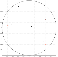
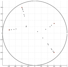
Figure 2. The poles of rational approximant to $f_{1}$ of degree 12 (left) and superimposed poles of rational approximants to $f_{1}$ of degrees 12 and 16 (right).

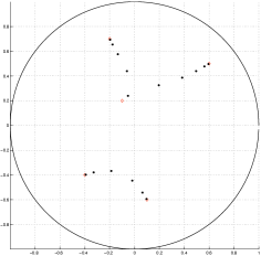
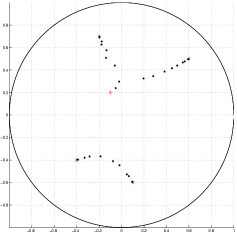
Figure 3. The poles of rational approximant to $f_{2}$ of degree 16 and superimposed poles of rational approximants to $f_{2}$ of degrees 13 and 16 (right).

On the figures diamonds depict the branch points of $f_{j}$, $j=1,2$, and disks denote the poles of the corresponding approximants.

References

- [1] V.M. Adamyan, D.Z. Arov, and M.G. Krein. Analytic properties of Schmidt pairs for a Hankel operator on the generalized Schur-Takagi problem. Math. USSR Sb., 15:31–73, 1971. English transl. in Math. USSR Sb. 15, 1971.
- [2] A. Antoulas. Approximation of Large-Scale Dynamical Systems, volume 6 of Advances in Design and Control. SIAM, Philadelphia, 2005.
- [3] A.I. Aptekarev. Sharp constant for rational approximation of analytic functions. Mat. Sb., 193(1):1–72, 2002. English transl. in Math. Sb. 193(1-2):1–72, 2002.
- [4] A.I. Aptekarev, A. Kuijlaars, and W. Van Assche. Asymptotics of Hermite-Padé rational approximants for two analytic functions with separated pairs of branch points (case of genus 0). Int. Math. Res. Pap., 2008.
- [5] L. Baratchart. Rational and meromorphic approximation in of the circle: system-theoretic motivations, critical points and error rates. In N. Papamichael, St. Ruscheweyh, and E. B. Saff, editors, Computational Methods and Function Theory, volume 11 of Approximations and Decompositions, pages 45–78, World Scientific Publish. Co, River Edge, N.J., 1999.
- [6] L. Baratchart. A remark on uniqueness of best rational approximants of degree 1 in on the circle. Electron. Trans. Numer. Anal., 25:54–66, 2006.
- [7] L. Baratchart, A. Ben Abda, F. Ben Hassen, and J. Leblond. Recovery of pointwise sources or small inclusions in 2D domains and rational approximation. Inverse Problems, 21:51–74, 2005.
- [8] L. Baratchart, M. Cardelli, and M. Olivi. Identification and rational approximation: a gradient algorithm. Automatica, 27(2):413–418, 1991.
- [9] L. Baratchart, J. Leblond, and J.-P. Marmorat. Inverse source problem in a 3D ball from best meromorphic approximation on 2D slices. Electron. Trans. Numer. Anal., 25:41–53, 2006.
- [10] L. Baratchart, F. Mandrèa, E.B. Saff, and F. Wielonsky. 2-D inverse problems for the Laplacian: a meromorphic approximation approach. J. Math. Pures Appl., 86:1–41, 2006.
- [11] L. Baratchart, E.B. Saff, and F. Wielonsky. A criterion for uniqueness of a critical points in rational approximation. J. Analyse Mathématique, 70:225–266, 1996.
- [12] L. Baratchart and F. Seyfert. An analog of AAK theory for . J. Funct. Anal., 191(1):52–122, 2002.
- [13] L. Baratchart and M. Yattselev. Asymptotic uniqueness of best rational approximants in of the unit circle to complex Cauchy transforms. In J. Arvesú, F. Marcellán, and A. Martínez Finkelshtein, editors, Recent Trends in Orthogonal Polynomials and Approximation Theory, Contemporary Mathematics. Amer. Math. Soc., 2010.
- [14] L. Baratchart and M. Yattselev. Convergent interpolation to Cauchy integrals over analytic arcs with Jacobi-type weights. Int. Math. Res. Not., 2010. Art. ID rnq 026, pp. 65.
- [15] V.I. Buslaev. On the Baker-Gammel-Wills conjecture in the theory of Padé approximants. Mat Sb., 193(6):25–38, 2002.
- [16] M. Clerc, J. Leblond, J.-P. Marmorat, and T. Papadopoulo. Source localization using rational approximation on plane sections. In preparation.
- [17] P. Deift. Orthogonal Polynomials and Random Matrices: a Riemann-Hilbert Approach, volume 3 of Courant Lectures in Mathematics. Amer. Math. Soc., Providence, RI, 2000.
- [18] P. Deift, T. Kriecherbauer, K.T.-R. McLaughlin, S. Venakides, and X. Zhou. Strong asymptotics for polynomials orthogonal with respect to varying exponential weights. Comm. Pure Appl. Math., 52(12):1491–1552, 1999.
- [19] J. Dieudonné. Foundations of Modern Analysis. Academic Press, New York, 1969.
- [20] P. Duren. Theory of Spaces. Dover Publications, Inc., New York, 2000.
- [21] O. Forster. Lectures on Riemann Surfaces, volume 81 of Graduate Texts in Mathematics. Springer-Verlag, New York, 4-th edition, 1999.
- [22] J. D. Fournier and J. Leblond, editors. Harmonic Analysis and Rational Approximation: Their Role in Signals, Control, and Dynamical Systems Theory, INRIA-CNRS-Observatoire de la Côte d’Azur, 2003. Proc. Summer School.
- [23] K. Glover. All optimal Hankel-norm approximations of linear multivariable systems and their –error bounds. Internat. J. Control, 39(6):1115–1193, 1984.
- [24] G.M. Goluzin. Geometric Theory of Functions of a Complex Variable, volume 26 of Translations of Math. Monographs. Amer. Math. Soc., Providence, RI, 1969.
- [25] A.A. Gonchar and E.A. Rakhmanov. Equilibrium distributions and the degree of rational approximation of analytic functions. Mat. Sb., 134(176)(3):306–352, 1987. English transl. in Math. USSR Sbornik 62(2):305–348, 1989.
- [26] J. Grimm. Rational approximation of transfer functions in the Hyperion software. Technical Report 4002, INRIA, September 2000.
- [27] V. Guillemin and A. Pollack. Differential Topology. Englewood Cliffs, N.J., Prentice-Hall, 1974.
- [28] E.J. Hannan and M. Deistler. The Statistical Theory of Linear Systems. Wiley, 1988.
- [29] V. Isakov. Inverse Source Problems, volume 34 of Math. Surveys Monogr. Amer. Math. Soc., Providence, RI, 1990.
- [30] S. Kamvissis, K.T.-R. McLaughlin, and P. Miller. Semiclassical soliton ensembles for the focusing nonlinear Schrödinger equation, volume 154 of Annals of Mathematics Studies. Princeton University Press, 2003.
- [31] A.B. Kuijlaars, K.T.-R. McLaughlin, W. Van Assche, and M. Vanlessen. The Riemann-Hilbert approach to strong asymptotics for orthogonal polynomials on . Adv. Math., 188(2):337–398, 2004.
- [32] G.V. Kuzmina. Modules of families of curves and quadratic differentials. Trudy Mat. Inst. Steklov, 139:1–240, 1980. English transl. in St. Petersburg Math. J., 9:455–507, 889–930, 1982.
- [33] S. Lang. Algebra. Number 211 in Graduate Texts in Mathematics. Springer, 2005.
- [34] J. Leblond, C. Paduret, S. Rigat, and M. Zghal. Source localization in ellipsoids by best meromorphic approximation in planar sections. Inverse Problems, 24(3), 2008.
- [35] A.L. Levin. The distribution of poles of rational functions of best approximation and related questions. Math. USSR Sbornik, 9(2):267–274, 1969.
- [36] D.S. Lubinsky. Rogers-Ramanujan and the Baker-Gammel-Wills (Padé) conjecture. Ann. of Math., 157(3):847–889, 2003.
- [37] N.K. Nikolskii. Treatise on the shift operator, volume 273 of Grundlehren der Math. Wissenschaften. Springer, 1986.
- [38] N.K. Nikolskii. Operators, Functions, and Systems: An Easy Reading. Parts I&II, volume 92 of Mathematical Surveys and Monographs. Amer. Math. Soc., Providence, RI, 2002.
- [39] O.G. Parfenov. Estimates of the singular numbers of a Carleson operator. Mat. Sb., 131(171):501–518, 1986. English. transl. in Math. USSR Sb. 59:497–514, 1988.
- [40] J.R. Partington. Interpolation, Identification and Sampling. Oxford University Press, Oxford, UK, 1997.
- [41] V.V. Peller. Hankel Operators and Their Applications. Springer Monographs in Mathematics. Springer-Verlag, New York, 2003.
- [42] E.A. Perevoznikova and E.A. Rakhmanov. Variation of the equilibrium energy and S-property of compacta of minimal capacity. Manuscript, 1994.
- [43] Ch. Pommerenke. Univalent Functions. Vandenhoeck & Ruprecht, Göttingen, 1975.
- [44] V.A. Prokhorov. Rational approximation of analytic functions. Mat. Sb., 184(2):3–32, 1993. English transl. in Russ. Acad. Sci., Sb., Math. 78(1):139–164, 1994.
- [45] T. Ransford. Potential Theory in the Complex Plane, volume 28 of London Mathematical Society Student Texts. Cambridge University Press, Cambridge, 1995.
- [46] P.A. Regalia. Adaptative IIR Filtering in Signal Processing and Control. Marcel Dekker, 1995.
- [47] E.B. Saff and V. Totik. Logarithmic Potentials with External Fields, volume 316 of Grundlehren der Math. Wissenschaften. Springer-Verlag, Berlin, 1997.
- [48] H. Stahl. Extremal domains associated with an analytic function. I, II. Complex Variables Theory Appl., 4:311–324, 325–338, 1985.
- [49] H. Stahl. Structure of extremal domains associated with an analytic function. Complex Variables Theory Appl., 4:339–356, 1985.
- [50] H. Stahl. Orthogonal polynomials with complex valued weight function. I, II. Constr. Approx., 2(3):225–240, 241–251, 1986.
- [51] H. Stahl. On the convergence of generalized Padé approximants. Constr. Approx., 5(2):221–240, 1989.
- [52] H. Stahl and V. Totik. General Orthogonal Polynomials, volume 43 of Encycl. Math. Cambridge University Press, Cambridge, 1992.
- [53] V. Totik. Personal communications.
- [54] J.L. Walsh. Interpolation and Approximation by Rational Functions in the Complex Domain, volume 20 of Colloquium Publications. Amer. Math. Soc., New York, 1935.