Improvements to model of projectile fragmentation

Abstract

In a recent paper Mallik we proposed a model for calculating cross-sections of various reaction products which arise from disintegration of projectile like fragment resulting from heavy ion collisions at intermediate or higher energy. The model has three parts: (1) abrasion, (2) disintegration of the hot abraded projectile like fragment (PLF) into nucleons and primary composites using a model of equilibrium statistical mechanics and (3) possible evaporation of hot primary composites. It was assumed that the PLF resulting from abrasion has one temperature $T$. Data suggested that while just one value of $T$ seemed adequate for most cross-sections calculations, it failed when dealing with very peripheral collisions. We have now introduced a variable $T=T(b)$ where $b$ is the impact parameter of the collision. We argue there are data which not only show that $T$ must be a function of $b$ but, in addition, also point to an approximate value of $T$ for a given $b$. We propose a very simple formula: $T(b)=D_{0}+D_{1}(A_{s}(b)/A_{0})$ where $A_{s}(b)$ is the mass of the abraded PLF and $A_{0}$ is the mass of the projectile; $D_{0}$ and $D_{1}$ are constants. Using this model we compute cross-sections for several collisions and compare with data.

I Introduction

In a recent paper Mallik we proposed a model of projectile mutifragmentation which was applied to collisions of Ni on Be and Ta at 140 MeV/nucleon and Xe on Al at 790 MeV/nucleon. The model gave reasonable answers for most of the cross-sections studied. The model requires integration over impact parameter. For a given impact parameter, the part of the projectile that does not directly overlap with the target is sheared off and defines the projectile like fragment(PLF). This is abrasion and appealing to the high enrgy of the beam, is calculated using straight line geometry. The PLF has $N_{s}$ neutrons,$Z_{s}$ protons and $A_{s}(=N_{s}+Z_{s})$ nucleons (the corresponding quantities for the full projectile are labelled $N_{0},Z_{0}$ and $A_{0}$). The abraded system $N_{s},Z_{s}$ has a temperture. In the second stage this hot PLF expands to one-third of the normal nuclear density. Assuming statistical equilibrium the break up of the PLF at a temperature $T$ is now calculated using the canonical thermodynamic model(CTM). The composites that result from this break up have the same temperature $T$ and can evolve further by sequential decay(evaporation). This is computed. Cross-sections can now be compared with experiment. The agreements were reasonable except for very peripheral collisions and it was conjectured in Mallik that the main reason for this discrepancy was due to the assumption of constant $T$ over all impact parameters.

Full details are provided in Mallik . Our aim here is to improve the model by incorporating an impact parameter dependence of $T=T(b)$. While we were led to this by computing the cross-sections of very large PLF’s (which can only result from very peripheral collisions), the effect of temperature dependence is accentuated in other experiments. In fact these experiments can be used, with some aid from reasonable models, to extract “experimental” values for temperature $T$ at each $b$. We spend considerable time studying this although our primary aim was and is the computation of cross-sections from a theoretical model.

II Basics of the Model

Consider the abrasion stage. The projectile hits the target. Use straight line geometry. We can then calculate the volume of the projectile that goes into the participant region (eqs.A.4.4 and A.4.5 of ref Dasgupta1 ). What remains in the PLF is $V$. This is a function of $b$. If the original volume of the projectile is $V_{0}$, the original number of neutrons is $N_{0}$ and the original number of protons is $Z_{0}$, then the average of neutrons in the PLF is $<N_{s}(b)>=[V(b)/V_{0}]N_{0}$ and the average number of protons is $<Z_{s}(b)>=[V(b)/V_{0}]Z_{0}$; $<N_{s}(b)>$ (and similarly $<Z_{s}(b)>$) is usually a non-integer. Since in any event only an integral number of neutrons (and protons) can appear in a PLF we need a prescription to get integral numbers. Let the two nearest integers to $<N_{s}(b)>$ be $N_{s}^{min}(b)$ and $N_{s}^{max}(b)=N_{s}^{min}(b)+1$. We assume that $P_{N_{s}}(b)$=the probability that the abraded system has $N_{s}$ neutrons is zero unless $N_{s}(b)$is either $N_{s}^{min}(b)$ or $N_{s}^{max}(b)$. Let $<N_{s}(b)>=N_{s}^{min}(b)+\alpha$ where $\alpha$ is less than 1. Then $P(N_{s}^{max}(b))=\alpha$ and $P(N_{s}^{min}(b)=1-\alpha$. Similar condions apply to $P_{Z_{s}}(b)$. The probability that a PLF with $N_{s}$ neutrons and $Z_{s}$ protons materializes from a collision at impact parameter $b$ is given by $P_{N_{s},Z_{s}}(b)=P_{N_{s}}(b)P_{Z_{s}}(b)$. Once this PLF is formed it will expand and break up into composites at a temperature $T$. We use CTM to obtain these. All the relevant details of CTM can be found in Mallik and Das . We will not repeat these here. There can be very light fragments, intermediate mass fragments (defined more precisely in the next section) and heavier fragments. As the fragments are at temperature $T$ it is possible some of these will sequentially decay thereby changing the final population which is measured experimentally. Details of evaporation can be found in Mallik and Chaudhuri1 .

III Arguments for $b$-dependence of Temperature

Experimental data on $M_{IMF}$ as a function of $Z_{bound}$ (see Fig.1 in Sfienti ) probably provide the strongest arguments for needing an impact parameter dependence of the temperature. Here $M_{IMF}$ is the average multiplicity of intermediate mass fragments (in this work those with $z$ between 3 and 20) and $Z_{bound}$=sum of all charges coming from PLF minus particles with $z$=1. For ease of arguments we will neglect, in this section, the difference between $Z_{bound}$ and $Z_{s}$, the total charge of all particles which originate from the PLF. A large value of $Z_{bound}$ (close to $Z_{0}$ of the projectile) signifies that the PLF is large and the collision is peripheral (large $b$) whereas a relatively smaller value of $Z_{bound}$ will imply more central collision (small $b$). For equal mass collision $Z_{bound}$ goes from zero to $Z_{0}$, the total charge of the projectile.

The following gross features of heavy ion collisions at intermediate energy are known. If the excitation energy (or the temperature) of the dissociating system is low then one large fragment and a small number of very light fragments emerge. The average multiplicity of IMF is very small. As the temperature increases, very light as well as intermediate mass fragments appear at the expense of the heavy fragment. The multiplicity $M_{IMF}$ will grow as a function of temperature, will reach a peak and then begin to go down as, at a high temperature, only light particles are dominant. For evidence and discussion of this see Tsang . For projectile fragmentation we are in the domain where $M_{IMF}$ rises with temperature. Now at constant temperature, let us consider what must happen if the dissociating system grows bigger. We expect $M_{IMF}$ will increase with the size of the dissociating system, that is, with $Z_{bound}$. Experimental data are quite different: $M_{IMF}$ initially increases, reaches a maximum at a particular value of $Z_{bound}$ and then goes down.

In Fig.1 we show two graphs for $M_{IMF}$, one in which the temperature is kept fixed (at 6.73 MeV) and another in which $T$ decreases linearly from 7.5 MeV (at $b$=0)to 3 MeV at $b_{max}$. The calculation is qualitative. The case considered is ¹²⁴Sn on ¹¹⁹Sn. CTM is used to calculate $M_{IMF}$ but evaporation is not included. Simlarly $Z_{bound}$ is $Z_{s}$ (no correction for $z=1$ particles). Fuller calculations will be shown later but the principal effects are all in the graphs. Keeping the temparature fixed makes $M_{IMF}$ go up all the way till $Z_{bound}$=$Z_{0}$ is reached. One needs the temperature to go down to bring down the value of $M_{IMF}$ as seen in experiment.

IV Use a model to extract $b$-dependence of Temperature

In our model we can use an iterative technique to deduce a temperature from experimental data of $M_{IMF}$ $\it{vs}$ $Z_{bound}$. Pick a $b$; abrasion gives a $<Z_{s}>$. Guess a temperature $T$. A full calculation with CTM and evaporation is now done to get a $Z_{bound}$ and $M_{IMF}$. This $Z_{bound}$ will be close to $<Z_{s}>$. If the guessed value of temperature is too low then the calculated value of $M_{IMF}$ will be too little for this value of $Z_{bound}$ when confronted with data. In the next iteration the temperature will be raised. If on the other hand, for the guess value of $T$, the calculated $M_{IMF}$ is too high, in the next iteration the temperature will be lowered. Of course when we change $T$, calculated $Z_{bound}$ will also shift but this change is smaller and with a small number of iterations one can approximately reproduce an experimental pair $Z_{bound},M_{IMF}$.

Experimental		Theoretical
$Z_{bound}$	$M_{IMF}$	$Z_{bound}$	$M_{IMF}$	b	Required T
				(fm)	(MeV)
11.0	1.421	11.080	1.424	2.912	6.398
15.0	1.825	15.094	1.818	3.625	6.108
20.0	2.145	19.984	2.131	4.4574	5.840
25.0	2.010	25.024	2.019	5.289	5.520
30.0	1.505	29.854	1.545	6.122	5.250
35.0	0.920	34.985	0.928	7.072	4.970
40.0	0.415	39.639	0.424	8.023	4.650
45.0	0.193	44.763	0.196	9.331	4.350
47.0	0.156	46.512	0.154	9.925	4.260
49.0	0.135	48.425	0.130	10.876	4.190

Table 1: Best fit and experimental values for ¹²⁴Sn on ¹¹⁹Sn. The first two columns are data from experiment. The next two columns are the values of $Z_{bound}$ and $M_{IMF}$ we get from our iterative procedure. These values are taken to be close enough to the experimental pair. These are obtained for a value of $b$ (fifth column) and a temperature $T$ (sixth column).

For the case of ¹²⁴Sn on ¹¹⁹Sn we provide Table I which demonstrates this. The first two columns are data from experiment. The next two columns are the values of $Z_{bound}$ and $M_{IMF}$ we get from our iterative procedure. These values are taken to be close enough to the experimental pair. These are obtained for a value of $b$ (sixth column) and a temperature $T$ (fifth column). Table II provides similar compilation for ¹⁰⁷Sn on ¹¹⁹Sn.

Experimental		Theoretical
$Z_{bound}$	$M_{IMF}$	$Z_{bound}$	$M_{IMF}$	b	Required T
				(fm)	(MeV)
15.0	1.690	14.816	1.583	3.886	6.200
20.0	1.923	19.865	1.906	4.698	5.740
21.0	1.984	21.207	1.976	4.930	5.705
25.0	1.749	24.913	1.758	5.510	5.320
30.0	1.079	30.356	1.075	6.438	4.900
35.0	0.581	35.252	0.602	7.366	4.600
40.0	0.223	40.123	0.225	8.410	4.210
45.0	0.201	44.676	0.199	9.802	4.100
47.0	0.201	47024	0.159	10.876	4.000

Table 2: Same as Table 1, except that here the projectile is ¹⁰⁷Sn instead of ¹²⁴Sn.

Having deduced once for all such “experimental data” of $T$ $\it{vs}$ $b$, one can try simple parametrisation like $T(b)=C_{0}+C_{1}*b+C_{2}*b^{2}...$. and see how well they fit the data. We show this for the two cases in Fig.2.

In Fig.3 using such parametrised versions of $T$ we compute $M_{IMF}$ $\it{vs}$ $Z_{bound}$ and compare with experimental data. Except for fluctuations in the values of $M_{IMF}$ for very low values of $Z_{bound}$ the fits are very good. We will return to the cases of fluctuations in a later section.

V Temperatures extracted from isotope populations

In the preceding sections we have extracted temperatures $T$ (combining data and model) at values of $b$ (equivalently at values of $Z_{bound}$). This is a new method for extracting temperature. A more standard way of extracting temperatures is the Albergo formula Albergo which has been widely used in the past (for a review see, for example, Dasgupta2 ; Pochodzalla ). In [Ogul , Figs.24 and 25] temperatures at selected values of $Z_{bound}/Z_{0}$ were extracted from populations in [^3,4He,^6,7Li] and [^7,9Be,^6,8Li] using Albergo formula. These temperatures are compared in Fig.4 with a typical temperature profile deduced here. It is gratifying to see that such different methods of extraction still give reasonable agreement.

VI Fluctuations in $M_{IMF}$ for small $Z_{bound}$

For small values of $Z_{bound}$ the measured $M_{IMF}$ shows considerable fluctuations as we go from one value of $Z_{bound}$ to another (see Fig.3). Our model does not reproduce these although general shapes are correct. Statistical models are not expected to show such fluctuations but let us get into some details which (a) give a clue how such fluctuations may arise and (b) why our model misses them. The reader who is not interested in such details can skip the rest of this section without loss of continuity.

For definiteness, consider the case of ¹²⁴Sn on ¹¹⁹Sn. By the definition of $IMF,(z>2)$, $M_{IMF}$ is 0 when $Z_{bound}$ is 2. Consider now $Z_{bound}=3$. The most direct way one can have this is if the PLF has $Z_{s}$=3. Taking very simplistic point of view, suppose, this also has $N_{s}=3$, that is, the PLF is ⁶Li. This is stable and we immediately get $M_{IMF}=1$. This is indeed the experimental value. The case of $Z_{bound}$=4 may arise if the PLF is $Z_{s}=4,N_{s}=4$, i.e., if the PLF is ⁸Be. But ⁸Be is unbound and will break up into two $\alpha$ particles which are not $IMF$’s. Thus $M_{IMF}$ drops to zero. In experiment this falls to about 0.3 rather than 0. The simple fact that ⁶Li (and an excited state of ⁶Li) is particle stable whereas the states of ⁸Be are not is not embedded in our liquid-drop model for ground state and Fermi-gas model for excited states. Our description gets better for larger nuclear systems but for very small systems quantum mechanics of nuclear forces causes rapid changes in properties as one goes from one excited state to another and one nucleus to another. Our model can not accommodate this.

Let us go back to the case of $Z_{s}$=3 and treat it more realistically. Using the abraison model, when $Z_{s}$ is 3, PLF can have $N_{s}$=3,4 and 5. Probabilities for higher and lower values of $N_{s}$ are small. Following our model we get $M_{IMF}\approx 0.94$ with $Z_{bound}$ slightly less than 3. When $Z_{s}$ is 4, significant probabilities occur for$N_{s}$=5,6 and 7. Following our model we get a small increase in $M_{IMF}$ with $Z_{bound}$ whereas experimentally $M_{IMF}$ falls. This discrepancy happens because in the Fermi-gas model there is very little difference between properties of ground and excited states of Li and Be whereas, in reality they are very different. A much more ambitious calculation for very small dissociating systems with $Z_{s}$ between 3 and 7 where we take binding energies and values of excited state energies from experiments (this becomes more and more unwieldy as $Z_{s}$ increases) is under way.

Fig.7 in ref Ogul shows that SMM calculations are able to reproduce the fluctuations faithfully. Actually in those calculations the occurrences of $Z_{s},N_{s}$ with associated $E_{x}$ are not calculated but guessed so that the ensemble produces the data as faithfully as possible. For further details how these calculations were done please refer to Botvina .

VII Towards a Universal Temperature Profile

Knowing the temperature profile $T=T(b)$ in one case, say ¹²⁴Sn on ¹¹⁹Sn, can we anticipate what $T=T(b)$ will be like in another case, say, ⁵⁸Ni on ⁹Be ? In both the cases $b_{min}$ is zero and $b_{max}$ is $R_{1}+R_{2}$ yet we can not expect the same functional form $T=T(b/b_{max})$ for both the cases. In the first case, near $b=0$ a small change in $b$ causes a large fractional change in the mass of the PLF whereas, for ⁵⁸Ni on ⁹Be, near $b$=0, a small change in $b$ causes very little change in the mass of the PLF. Thus we might expect the temperature to change more rapidly in the first case near $b$=0, whereas, in the second case, the temperature may change very little since not much changed when $b$ changed a little. In fact, for Ni on Be, transport model calculations, HIPSE (Heavy Ion Phase Space Exploration) and AMD (Antisymmetrised Molecular Dynamics) find that starting from $b$=0, excitation energy/per particle changes very little in the beginning Mocko2 . In terms of our model, this would mean that for Ni on Be, $T$ would be slow to change in the beginning.

We might argue that a measure of the wound that the projectile suffers in a heavy ion collision is $1.0-A_{s}/A_{0}$ and that the temperature depends upon the wound. Thus we should expect $T=T(A_{s}(b)/A_{0})$. Just as we can write $T(b)=C_{0}+C_{1}*b+C_{2}*b^{2}+...$ so also we could expand in powers of $A_{s}(b)/A_{0}$,i.e., $T(b)=D_{0}+D_{1}(A_{s}(b)/A_{0})+D_{2}(A_{s}(b)/A_{0})^{2}+...$ We try such fits to the “experimental” temperature profile given in Tables I and II. From $b$ we deduce $A_{s}(b)/A_{0}$ and plot $T$ as a function of $A_{s}(b)/A_{0}$. A linear fit appears to be good enough (Fig.5).

The specification that $T(b)=D_{0}+D_{1}(A_{s}(b)/A_{0})$ has profound consequences. This means the temperature profile $T(b/b_{max})$ of ¹²⁴Sn on ¹¹⁹Sn is very different from that of ⁵⁸Ni on ⁹Be. In the first case $A_{s}(b)/A_{0}$ is nearly zero for $b=b_{min}$=0 whereas in the latter case $A_{s}(b)/A_{0}$ is $\approx 0.6$ for $b=b_{min}$=0. For $D_{0}$=7.5 MeV and $D_{1}$=-4.5 MeV, the temperature profiles are compared in Fig.6. Even more remarkable feature is that the temperature profile of ⁵⁸Ni on ⁹Be is so different from the temperature profile of ⁵⁸Ni on ¹⁸¹Ta. In the latter case $b_{min}=R_{Ta}-R_{Ni}$ and beyond $b_{min}$, $A_{s}(b)/A_{0}$ grows from zero to 1 for $b_{max}$. This is very similar to the temperature profile of ¹²⁴Sn on ¹¹⁹Sn.

VIII Formulae for cross-sections

Now that we have established that temperature $T$ should be considered impact parameter $b$ dependent, let us write down how cross-sections should be evaluated. We first start with abrasion cross-section. In eq.(1) of Mallik , the abrasion cross-section was written as

$$\sigma_{a,N_{s},Z_{s}}=2\pi\int bdbP_{N_{s},Z_{s}}(b)$$ (1)

where $P_{N_{s},Z_{s}}(b)$ is the probability that a PLF with $N_{s}$ neutrons and $Z_{s}$ protons emerges in collision at impact parameter $b$. Actually there is an extra parameter that needs to be specified. The complete labelling is $\sigma_{a,N_{s},Z_{s},T}$ if we assume that irrespective of the value of $b$, the PLF has a temperature $T$. Here we have broadened this to the more general case where the temperature is dependent on the impact parameter $b$. Thus the PLF with $N_{s}$ neutrons and $Z_{s}$ protons will be formed in a small range of temperature (as the production of a particular $N_{s},Z_{s}$ occurs in a small range of $b$).

To proceed, let us discretize. We divide the interval $b_{min}$ to $b_{max}$ into small segments of length $\Delta b$. Let the mid-point of the $i$-th bin be $<b_{i}>$ and the temperature for collision at $<b_{i}>$ be $T_{i}$. Then

$$\sigma_{a,N_{s},Z_{s}}=\sum_{i}\sigma_{a,N_{s},Z_{s},T_{i}}$$ (2)

where

$$\sigma_{a,N_{s},Z_{s},T_{i}}=2\pi<b_{i}>\Delta bP_{N_{S},Z_{s}}(<b_{i}>)$$ (3)

PLF’s with the same $N_{s},Z_{s}$ but different $T_{i}$’s are treated independently. The rest of the calculation proceeds as in Mallik . If, after abrasion, we have, a system $N_{s},Z_{s}$ at temperature $T_{i}$, CTM allows us to compute the average population of the composite with neutron number $n$, proton number $z$ when this system breaks up (this composite is at temperature $T_{i}$). Denote this by $M_{n,z}^{N_{s},Z_{s},T_{i}}$. It then follows, summing over all the abraded $N_{s},Z_{s}$ that can yield $n,z$ the primary cross-section for $n,z$ is

$$\sigma_{n,z}^{pr}=\sum_{N_{s},Z_{s},T_{i}}M_{n,z}^{N_{s},Z_{s},T_{i}}\sigma_{a,N_{s},Z_{s},T_{i}}$$ (4)

Finally, evaporation from these composites $n,z$ at temperatures $T_{i}$ is considered before comparing with experimental data.

IX Cross-sections for different reactions

We will now show some results for cross-sections using our model and compare with experimental data. We first show results for ¹²⁴Sn on ¹¹⁹Sn and ¹⁰⁷Sn on ¹¹⁹Sn at 600 MeV/nucleon beam energy. The experimental data are plotted in Ogul and the data were given to us, thanks to Prof. Trautmann. The differential charge distributions and isotopic distributions for ¹⁰⁷Sn on ¹¹⁹Sn and ¹²⁴Sn on ¹¹⁹Sn were theoretically calculated using $T(b)=C_{0}+C_{1}b$ and and also $T(b)=D_{0}+D_{1}(A_{s}(b)/A_{0})$. So long as the temperature values at the two end points of $b$ are the same, the answers did not differ much. In Fig.7 we have shown results for $T$ varying linearly with $b$ with $T_{max}=7.5$MeV and $T_{min}$=3 MeV. At each $Z_{bound}$, the charge distribution and isotopic distributions are calculated separately and finally integrated over different $Z_{bound}$ ranges. The differential charge distributions are shown in Fig.7 for different intervals of $Z_{bound}/Z_{0}$ ranging between $0.0$ to $0.2$, $0.2$ to $0.4$, $0.4$ to $0.6$, $0.6$ to $0.8$ and $0.8$ to $1.0$. For the sake of clarity the distributions are normalized with different multiplicative factors. At peripheral collisions (i.e. $0.8{\leq}Z_{bound}/Z_{0}{\leq}1.0$) due to small temperature of the projectile spectator, it breaks into one large fragment and small number of light fragments, hence the charge distribution shows $U$ type nature. But with the decrease of impact parameter the temperature increases, the projectile spectator breaks into large number of fragments and the charge distributions become steeper. In Figs.8 and 9 the integrated isotopic distributions over the range $0.2{\leq}Z_{bound}/Z_{0}{\leq}0.8$ for Beryllium, Carbon, Oxygen and Neon are plotted and compared with the experimental result for ¹⁰⁷Sn on ¹¹⁹Sn and ¹²⁴Sn on ¹¹⁹Sn reaction respectively.

Rest of the cross-sections shown all use $T(b)=7.5$MeV-$(A_{S}(b)/A_{0})4.5$MeV. First, in Fig. 10 the calculations of Fig. 7 are redone but with the above parametrization. Next we look at data for ⁵⁸Ni on ⁹Be and ¹⁸¹Ta at beam energy 140 MeV/nucleon done at Michigan State University. The data were made available to us by Dr.Mocko (Mocko, Ph.D. thesis). Calculations were also done with ⁶⁴Ni as beam. Those results agree with experiment equally well but are not shown here for brevity. The results for ⁵⁸Ni on ⁹Be and ⁵⁸Ni on ¹⁸¹Ta are shown in Figs.11 to 14. The experimental data are from Mocko2 . The chief difference from results shown in Mallik is that we are able to include data for very peripheral collisions. Next we look at some older data from ¹²⁹Xe on ²⁷Al at 790 MeV/nucleon Reinhold . Results are given in Figs. 15 and 16.

The parametrization $T(b)=7.5$MeV-$(A_{s}(b)/A_{0})4.5$MeV was arrived at by trying to fit many reaction cross-section data. Better fit for $M_{IMF}$ vs. $Z_{bound}$ for Sn isotopes is found with slightly different values: $T(b)=7.2$MeV-$(A_{s}(b)/A_{0})3.2$MeV.

X Summary and Discussion

We have shown that there are specific experimental data in projectile fragmentation which clearly establish the need to introduce an impact parameter dependence of temperature $T$ in the PLF formed. Combining data and a model one can establish approximate values of $T=T(b)$. The model for cross-sections has been extended to incorporate this temperature variation. This has allowed us to investigate more peripheral collisions. In addition, the impact parameter dependence of temperature appears to be very simple: $T(b)=D_{0}+D_{1}(A_{s}(b)/A_{0})$ where $D_{0}$ and $D_{1}$ are constants, $A_{s}(b)$ is the mass of the PLF and $A_{0}$ is the mass of the projectile. With this model, we plan to embark upon an exhaustive study of available data on projectile fragmentation.

XI Acknowledgments

This work was supported in part by Natural Sciences and Engineering Research Council of Canada. The authors are thankful to Prof. Wolfgang Trautmann and Dr. M. Mocko for access to experimental data. S. Mallik is thankful for a very productive and enjoyable stay at McGill University for part of this work. S. Das Gupta thanks Dr. Santanu Pal for hospitality at Variable Energy Cyclotron Centre at Kolkata.

Figure 1: (Color Online) Mean multiplicity of intermediate-mass fragments $M_{IMF}$ (after multifragmentation stage), as a function of projectile spectator charge for ¹²⁴Sn on ¹¹⁹Sn reaction calculated at a fixed temperature $T$=6.73 MeV (black solid line) and at a linearly decreasing temperature from 7.5 MeV at $b$=0 to 3 MeV at $b_{max}$ (red dotted line). The ordinate is labelled $<M_{IMF}>^{pri}$ as the effect of evaporation is not included.

Figure 2: (Color Online) Impact parameter dependence of temperature for ¹⁰⁷Sn on ¹¹⁹Sn (left panels) and ¹²⁴Sn on ¹¹⁹Sn reactions (right panels). The red squires in the upper panels represent the extracted temperatures (sixth column of table-I and II) and the blue dotted lines are linearly decreasing temperature profile from 7.5 MeV to 3 MeV. The blue dotted lines of middle and lower panels represent fitting of extracted temperatures (red squires) with $T(b)=C_{0}+C_{1}*b$ and $T(b)=C_{0}+C_{1}*b+C_{2}*b^{2}$ equation respectively. The unit of $C_{0}$ is MeV, $C_{1}$ is MeVfm^-1 and $C_{2}$ is MeVfm^-2.

Figure 3: (Color Online) Mean multiplicity of intermediate-mass fragments $M_{IMF}$, as a function of $Z_{bound}$ for ¹⁰⁷Sn on ¹¹⁹Sn (left panel) and ¹²⁴Sn on ¹¹⁹Sn (right panel) reaction calculated using linearly decreasing temperature from 7.5 MeV to 3 MeV (red solid lines) and $T(b)=C_{0}+C_{1}*b+C_{2}*b^{2}$ profile (blue dotted lines). The experimental results are shown by the black dashed lines.

Figure 4: (Color Online) Comparison of theoretically used temperature profiles (i) temperature decreasing linearly with impact parameter from 7.5 MeV to 3 MeV (red solid lines), (ii)$T(b)=C_{0}+C_{1}*b+C_{2}*b^{2}$ fitting temperature (blue dotted lines) with that deduced by Albergo formula from experimental data (black points with error bars) for ¹⁰⁷Sn on ¹¹⁹Sn (left panel) and ¹²⁴Sn on ¹¹⁹Sn (right panel).

Figure 5: (Color Online) Fitting of extracted temperatures (red squires) with $T(b)=D_{0}+D_{1}(A_{s}(b)/A_{0})$ (blue dotted lines in upper panels) and $T(b)=D_{0}+D_{1}(A_{s}(b)/A_{0})+D_{2}(A_{s}(b)/A_{0})^{2}$ profile (blue dotted lines in lower panels) for ¹⁰⁷Sn on ¹¹⁹Sn (left panels) and ¹²⁴Sn on ¹¹⁹Sn (right panels). The units of $D_{0}$, $D_{1}$ and $D_{2}$ are MeV.

Figure 6: (Color Online) Temperature profile for ⁵⁸Ni on ⁹Be (black solid line), ⁵⁸Ni on ¹⁸¹Ta (red dotted line) and ¹²⁴Sn on ¹¹⁹Sn (blue dashed line) by considering $T=7.5-4.5(A_{s}(b)/A_{0})$

Figure 7: (Color Online) Theoretical total charge cross-section distribution (red solid lines) for ¹⁰⁷Sn on ¹¹⁹Sn (left panel) and ¹²⁴Sn on ¹¹⁹Sn reaction (right panel) sorted into five intervals of $Z_{bound}/Z_{0}$ ranging between $0.0$ to $0.2$, $0.2$ to $0.4$, $0.4$ to $0.6$, $0.6$ to $0.8$ and $0.8$ to $1.0$ with different multiplicative factors $10^{-4}$, $10^{-2}$, $10^{0}$, $10^{2}$, $10^{5}$ respectively. The experimental data are shown by black dashed lines. Theoretical calculation is done using linearly decreasing temperature from 7.5 MeV at $b$=0 to 3 MeV at $b_{max}$.

Figure 8: (Color Online) Theoretical isotopic cross-section distribution (circles joined by dashed lines) for ¹⁰⁷Sn on ¹¹⁹Sn reaction summed over $0.2{\leq}Z_{bound}/Z_{0}{\leq}0.8$. The experimental data are shown by black squires. Theoretical calculation is done using linearly decreasing temperature from 7.5 MeV at $b$=0 to 3 MeV at $b_{max}$.

Figure 9: (Color Online) Same as Fig. 8, except that here the projectile is ¹²⁴Sn instead of ¹⁰⁷Sn.

Figure 10: (Color Online) Same as Fig. 7 except that here the temperature profile is $T(b)=7.5MeV-(A_{S}(b)/A_{0})4.5MeV$ instead of linearly decreasing temperature from 7.5 MeV at $b$=0 to 3 MeV at $b_{max}$

Figure 11: (Color Online) Total mass (left panel) and total charge (right panel) cross-section distribution for the ⁵⁸Ni on ⁹Be reaction. The left panel shows the cross-sections as a function of the mass number, while the right panel displays the cross-sections as a function of the proton number. The theoretical calculation is done using temperature decreasing linearly with $A_{s}/A_{0}$ from 7.5 MeV to 3.0 MeV (dashed line) and compared with the experimental data (solid line).

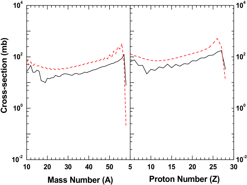
Figure 12: (Color Online) (Color Online) Same as Fig. 11 except that here the target is ¹⁸¹Ta instead of ⁹Be.

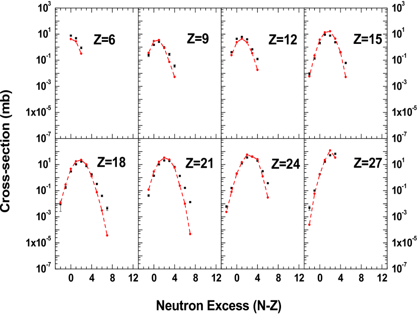
Figure 13: (Color Online) Theoretical isotopic cross-section distribution (circles joined by dashed lines) for ⁵⁸Ni on ⁹Be reaction compared with experimental data (squares with error bars).

Figure 14: (Color Online) Same as Fig. 13 except that here the target is ¹⁸¹Ta instead of ⁹Be.

Figure 15: (Color Online) Total charge cross-section distribution for the ¹²⁹Xe on ²⁷Al reaction. The theoretical calculation is done using temperature decreasing linearly with $A_{s}/A_{0}$ from 7.5 MeV to 3.0 MeV (dashed line) and compared with the experimental data (solid line).

Figure 16: (Color Online) Theoretical isotopic cross-section distribution (circles joined by dashed lines) for ¹²⁹Xe on ²⁷Al reaction compared with experimental data (squares with error bars).

References

- (1) S. Mallik, G. Chaudhuri and S. Das Gupta, Phys. Rev. C 83, 044612 (2011).
- (2) S. Das Gupta and A. Z. Mekjian,Phys. Rep. 72, 131 (1981).
- (3) C. B. Das, S. Das Gupta, W. G. Lynch, A. Z. Mekjian and M. B. Tsang, Phys. Rep. 406, 1 (2005).
- (4) G. Chaudhuri, S. Mallik, Nucl. Phys. A 849, 190 (2011).
- (5) C. Sfienti et al., Phys. Rev. Lett. 102, 152701 (2009).
- (6) M. B. Tsang et al., Phys. Rev. Lett. 71, 1502 (1993).
- (7) R. Ogul et al.,Phys. Rev C 83,024608(2011)
- (8) A. S. Botvina et al., Nucl. Phys. A 584, 737 (1995).
- (9) S. Albergo et al., Il Nuovo Cimento 89, A1(1985)
- (10) S. Das Gupta, A. Z. Mekjian and M. B. Tsang, Advances in Nuclear Physics, Vol.26,89(2001)edited by J. W. Negele and E. Vogt, Plenum Publishers, New York.
- (11) J. Pochodzalla and W. Trautmann, Isospin Physics in Heavy-Ion Collisions at Intermediate Energies, 451(2001) edited by B-A Li and W. U. Schrder, Nova Science Publishers,Inc, Huntington, New York.
- (12) M. Mocko,Ph.D. thesis, Michigan State University, 2006.
- (13) M. Mocko et al., Phys. Rev. C 78, 024612 (2008).
- (14) J. Reinhold et al., Phys. Rev. C 58, 247 (1998).