Pion-photon transition form factor using light-cone sum rules:
theoretical results, expectations, and a global-data fit

Abstract

A global fit to the data from different collaborations (CELLO, CLEO, BaBar) on the pion-photon transition form factor is carried out using light-cone sum rules. The analysis includes the next-to-leading QCD radiative corrections and the twist-four contributions, while the main next-to-next-to-leading term and the twist-six contribution are taken into account in the form of theoretical uncertainties. We use the information extracted from the data to investigate the pivotal characteristics of the pion distribution amplitude. This is done by dividing the data into two sets: one containing all data up to 9 GeV², whereas the other incorporates also the high-$Q^{2}$ tail of the BaBar data. We find that it is not possible to accommodate into the fit these BaBar data points with the same accuracy and conclude that it is difficult to explain these data in the standard scheme of OCD.

I Form factor $\mathbf{F^{\gamma^{*}\gamma^{*}\pi}}$ in collinear QCD

One of the most studied exclusive processes within QCD, based on collinear factorization, is the pion-photon transition form factor with both photon virtualities being sufficiently large, see BL89 for a review. The transition form factor is defined by the correlator of two electromagnetic currents

$$\int\!d^{4}z\,e^{-iq_{1}\cdot z}\langle\pi^{0}(P)\mid T\{j_{\mu}(z)j_{\nu}(0)\}\mid 0\rangle$$

$$=i\epsilon_{\mu\nu\alpha\beta}q_{1}^{\alpha}q_{2}^{\beta}F^{\gamma^{*}\gamma^{*}\pi}(Q^{2},q^{2})$$ (1)

with $Q^{2}\equiv-q_{1}^{2}>0$, $q^{2}\equiv-q_{2}^{2}\geq 0$, and can be reexpressed in the form ER80

$$F^{\gamma^{*}\gamma^{*}\pi}(Q^{2},q^{2}) \!\!\!\!=\!\!\!\! N\,\int_{0}^{1}\!dx\,T(Q^{2},q^{2},\mu^{2}_{\rm F},x)\,$$ (2)

$$\times\ \varphi^{(2)}_{\pi}(x,\mu^{2}_{\rm F})+O\left(\delta^{2}/Q^{4}\right)\,,$$

by virtue of collinear factorization, assuming that the photon momenta are sufficiently large $Q^{2},q^{2}\gg m_{\rho}^{2}$. Here $N=\sqrt{2}/3f_{\pi}$, $f_{\pi}=132$ MeV is the pion-decay constant, and $\delta^{2}$ is the twist-four coupling. Then, the quark-gluon sub-processes, formulated in terms of the hard-scattering amplitude of twist-two, $T$, can be computed order-by-order of QCD perturbation theory: $T=T_{0}+a_{s}T_{1}+a_{s}^{2}T_{2}+\ldots$. The radiative corrections in next-to-leading order (NLO), $T_{1}$, have been obtained in DaCh81 , the $\beta_{0}$–part of the contribution at the next-to-next-to-leading order level (NNLO_β), encoded in the amplitude $T_{2}$, i.e., $\beta_{0}\cdot T_{2\beta}$, was calculated in MMP02 .

The binding effects are separated out and absorbed into a universal pion distribution amplitude (DA) of twist-two, $\varphi^{(2)}_{\pi}(x,\mu^{2})$, defined Rad77 by the matrix element

$$\langle 0|\bar{q}(z)\gamma_{\nu}\gamma_{5}[z,0]q(0)|\pi(P)\rangle\Big{|}_{z^{2}=0}\!\!\! = \!iP_{\nu}f_{\pi}\int_{0}^{1}dxe^{ix(z\cdot P)}$$ (3)

$$\times\varphi^{(2)}_{\pi}(x,\mu^{2}_{\rm F})\!\,.$$

The variation of $\varphi^{(2)}_{\pi}(x,\mu^{2}_{\rm F})$ with the factorization scale $\mu^{2}_{\rm F}$ is controlled by the Efremov–Radyushkin–Brodsky–Lepage (ERBL) evolution equation ER80 ; moreover the Gegenbauer harmonics $\{\psi_{n}(x)\}$ constitute the leading-order (LO) eigenfunctions of this equation. Therefore, it is useful to expand the pion DA in terms of these harmonics:

$$\varphi^{(2)}_{\pi}(x,\mu^{2})=\psi_{0}(x)+\sum\nolimits_{n=2,4,\ldots}a_{n}\left(\mu^{2}\right)\psi_{n}(x)\,,$$ (4)

where $\psi_{n}(x)\!=\!6x(1-x)C^{3/2}_{n}(2x-1)$ and $\varphi^{\rm as}(x)\!=\!\psi_{0}(x)\!=\!6x(1-x)$ is the asymptotic pion DA ER80 . The nonperturbative information is contained in the coefficients $a_{n}\left(\mu^{2}\right)$ with ($n\geq 2$) that have to be modeled or extracted form the data, including evolution effects to account for their $\mu^{2}$-dependence. They are usually reconstructed from the moments $\langle\xi^{N}\rangle_{\pi}\equiv\int_{0}^{1}dx(2x-1)^{N}\varphi_{\pi}^{(2)}(x,\mu^{2})$ with $\langle\xi^{0}\rangle_{\pi}=1$ that can be determined by employing, e.g., QCD sum rules (SR)s CZ84 . We use here the pion DA proposed before in the framework of improved QCD SRs with nonlocal condensates (NLC-SRs) BMS01 that yield a “bunch” of admissible pion DAs with two harmonics that fix the coefficients $a_{2}$ and $a_{4}$.

II Light-cone sum rules for the process $\mathbf{\gamma^{*}(Q^{2})\gamma(q^{2}\simeq 0)\to\pi^{0}}$

The pion-photon transition involving two highly off-shell photons is not easily accessible to experiment. Experimental information is mostly available for an asymmetric photon kinematics, with one of the photons having a virtuality close to zero $q^{2}\to 0$ CELLO91 ; CLEO98 ; BaBar09 . The calculation of this transition form factor within perturbative QCD is a precarious step because the quasi-real photon is emitted at large distances and has, therefore, a hadronic content calling for the application of nonperturbative techniques. An appropriate method is provided by light-cone sum rules (LCSRs) Kho99 that supplements QCD perturbation theory with a dispersion relation for $F^{\gamma^{*}\gamma^{*}\pi}$ in the variable $q^{2}$, taking then $q^{2}\to 0$, whereas the large variable $Q^{2}$ is kept fixed. Thus, one has

$$F^{\gamma^{*}\gamma^{*}\pi}\left(Q^{2},q^{2}\right)=N\,\int_{0}^{\infty}\!\!ds\,\frac{\rho\left(Q^{2},s\right)}{s+q^{2}}\,,$$ (5)

with the physical spectral density $\rho(Q^{2},s)$ approaching at large $s$ the perturbative one:

$$\rho^{\rm PT}(Q^{2},s)=\frac{1}{\pi}{\rm\mathbf{Im}}\left[F^{\gamma^{*}\gamma^{*}\pi}\left(Q^{2},-s-i\varepsilon\right)/N\right].$$ (6)

Using quark-hadron duality, we obtain the following LCSR Kho99 :

$$\!\!\!\!Q^{2}F^{\gamma^{*}\gamma\pi}\left(Q^{2}\right)=\frac{Q^{2}}{m_{\rho}^{2}}\int_{x_{0}}^{1}\!\!\frac{dx}{x}\exp\left(\frac{m_{\rho}^{2}-Q^{2}\bar{x}/x}{M^{2}}\right)$$

$$\times N\,\bar{\rho}(Q^{2},x)+\int_{0}^{x_{0}}\frac{dx}{\bar{x}}N\,\bar{\rho}(Q^{2},x)$$ (7)

with the spectral density $\bar{\rho}(Q^{2},x)=(Q^{2}+s)\rho^{\rm PT}(Q^{2},s)$, where $s=\bar{x}Q^{2}/x$ and $x_{0}=Q^{2}/(Q^{2}+s_{0})$. Note that the first term in (7) is associated with the hadronic content of a quasi-real photon at low $s\leq s_{0}$, whereas the second term reproduces its point-like behavior at the higher value $s>s_{0}$. We adjust the hadronic threshold in the vector-meson channel to the value $s_{0}=1.5$ GeV², using $m_{\rho}=0.77$ GeV PDG2010 . We avoid to vary the Borel parameter $M^{2}$ in (7) and specify its value by virtue of $M^{2}=M_{\rm 2-pt}^{2}/\langle{x}\rangle_{Q^{2}}$ entering the two-point QCD sum rule for the $\rho$-meson with $M_{\rm 2-pt}^{2}\in[0.5\div 0.8]$ GeV², where $\langle{x}\rangle_{Q^{2}}$ denotes some average value of $x$ (at fixed $Q^{2}$) in the integration region for the first integral on the right-hand side of Eq. (7) Kho99 ; BMPS11 , i.e., $x_{0}(Q^{2})<\langle{x}\rangle_{Q^{2}}<1$.

III Main ingredients of the LCSRs and conditions of the data analysis

It is convenient to invent for each term of the harmonics $\psi_{n}$, a partial spectral density according to the definition (6) for the twist-two part MS09 , $\rho_{n}^{(i)}(Q^{2},s)\!=\!\frac{\mathbf{Im}}{\pi}\left[\left(T_{i}\otimes\psi_{n}\right)(Q^{2},-s-i\varepsilon)\right]$. The general solution for $\bar{\rho}^{(1)}_{n}$ in NLO was obtained in MS09 and corrected later (third line) in ABOP10 :

$$\frac{1}{C_{\rm F}}\bar{\rho}^{(1)}_{n}\left(\frac{Q^{2}}{\mu^{2}_{\rm F}};x\right)=\left\{-3\left[1+v^{b}(n)\right]+\frac{\pi^{2}}{3}-\ln^{2}\left(\frac{\bar{x}}{x}\right)\right.$$

$$\left.+2v(n)\ln\left(\frac{\bar{x}}{x}\frac{Q^{2}}{\mu^{2}_{\rm F}}\right)\right\}\psi_{n}(x)$$

$$\!\!\!\!\!\!\!\!\!\!\!\!\!\!-2\!\left[\sum^{n}_{l=0,2,\ldots}\!\!\!G_{nl}\psi_{l}(x)+v(n)\!\left(\sum^{n}_{l=0,1,\ldots}\!\!\!b_{nl}\psi_{l}(x)-3\bar{x}\!\right)\!\right],$$ (8)

with $v(n),v^{b}(n)$ being the eigenvalues of LO ERBL equations, whereas $G_{nl}$ and $b_{nl}$ are calculable triangular matrices (see MS09 ; ABOP10 for details).

The inclusion of the NNLO_β contribution to the main partial spectral density $\beta_{0}\cdot\bar{\rho}^{(2\beta)}_{0}$, derived from $\beta_{0}\cdot T_{2\beta}$ MMP02 , was realized in MS09 ; BMPS11 . It turns out that, taken together with the positive effect of a more realistic Breit-Wigner ansatz for the meson resonance MS09 instead of using a $\delta$-function, i.e., $\delta(s-m^{2}_{\rho})F^{\gamma^{*}\rho\pi}$, as in (7), it is negative and about –7% at small $Q^{2}\sim 2$ GeV², decreasing rapidly to –2.5% at $Q^{2}\geq 6$ GeV². Here the results are expanded to include the first three harmonics.

On the other hand, the twist-six contribution to $F^{\gamma^{*}\gamma\pi}$ was recently computed in ABOP10 using $M^{2}\sim 1.5$ GeV² and found to be very small. Using instead the more moderate value $M^{2}\sim 0.75$ GeV² BMPS11 , it turns out to have almost the same magnitude as the NNLO_β term, but with the opposite sign.

As already mentioned, we use here the BMS bunch of pion DAs with the central point $a_{2}^{\text{BMS}}(1\text{GeV}^{2})=0.20$ and $a_{4}^{\text{BMS}}(1\text{GeV}^{2})=-0.14$ (termed the BMS model) BMS01 . These pion DAs have their endpoints at $x=0$ and $x=1$ suppressed—even relative to the asymptotic pion DA—and are in good agreement with the CLEO data on the pion-photon transition form factor as well as with the data for other pion observables BMS02 ; BMS03 ; BMS05lat .

The key features of our data-analysis are the following: (i) The NLO radiative corrections in the spectral density are included via the corrected expression (8), emphasizing that this error does not affect our previous results in BMS02 ; BMS03 ; BMS05lat ; MS09 . The so-called default renormalization-scale setting is adopted and, accordingly, the factorization and the renormalization scales have been identified with the large photon virtuality $Q^{2}$. (ii) The twist-four contribution is taken into account using for the effective twist-four DA the asymptotic form $\varphi_{\pi}^{(4)}(x,\mu^{2})=(80/3)\,\delta^{2}(\mu^{2})\,x^{2}(1-x)^{2}$ Kho99 ; BF89 . We also admit a significant variation of the parameter $\delta^{2}=0.19$ GeV² in the range 0.15 GeV² to $0.23$ GeV², referring for details to BMS03 , and taking into account its evolution with $\mu^{2}$. Using a nonasymptotic form for $\varphi_{\pi}^{(4)}$ would not change these results significantly BMS05lat ; Ag05b . (iii) The evolution effects of the coefficients $a_{n}$ are also included in NLO, employing the QCD scale parameters $\Lambda_{\rm QCD}^{(3)}=370$ MeV and $\Lambda_{\rm QCD}^{(4)}=304$ MeV, conforming with the NLO estimate $\alpha_{s}(M_{Z}^{2})=0.118$ PDG2010 . (iv) The NNLO_β radiative correction to the LCSR form factor MS09 ; BMPS11 , Eq. (7), is incorporated together with the twist-six term, computed in ABOP10 , in terms of theoretical uncertainties. To be precise, the calculation of the NNLO_β term involves only the convolution of the hard-scattering amplitude $T_{\beta}$ with the DA based on the three lowest harmonics. This treatment makes sense due to the fact that for the average value of $M^{2}(Q^{2})\sim 0.75$ GeV², these two contributions almost mutually cancel and the net result is small—see Fig.1.

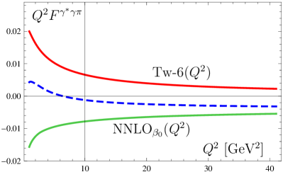
Figure 1: Twist-six contribution (upper solid line in red) and NNLO_β contribution (lower solid line in green), obtained with the BMS model, and their sum (dashed blue line).

In fact, it decreases with $Q^{2}$ from $+0.004$ at $Q^{2}=1$ GeV²—where the twist-six term dominates—down to $-0.003$ at $Q^{2}=40$ GeV²—where the NNLO_β correction starts prevailing. This particular behavior applies only to the moderate value of the Borel parameter $M^{2}=0.75$ GeV² BMPS11 , while for the larger value $M^{2}=1.5\pm 0.5$ GeV², used in ABOP10 , the twist-six term would be much smaller and the net result would be everywhere negative and almost constant: $\approx-0.004$.

IV Data Analysis

Here we overview our fit procedure of all available experimental data on the pion-photon transition form factor $F^{\gamma^{*}\gamma\pi}$, within the framework of LCSRs, as worked out in BMPS11 . The main goal of the fit is to extract the pion DA—the main low-energy pion characteristic—best compatible with all the data. This is done fitting the form factor by varying the pion DA in terms of the Gegenbauer coefficients $a_{n}$. To reveal the particular role of the new high-$Q^{2}$ BaBar data in the fit, we perform our analysis utilizing two different data sets. The first set (set-1) contains all available data from CELLO CELLO91 , CLEO CLEO98 , and BaBar BaBar09 that belong to the $Q^{2}$-window $[1\div 9]$ Gev². The second set (set-2) comprises all data in the range $[1\div 40]$ GeV². First, we define the optimal number of Gegenbauer harmonics necessary to model the pion DA. Second, we determine the fiducial regions of the corresponding coefficients $a_{n}$. Third, we relate these regions with the pion DA and its characteristics: profiles, derivatives at the origin, and its moments. Finally, we confront the obtained results with the data of set-1 and set-2.

IV.1 How many harmonics should be taken into account?

To answer this question, we confront the dependence of the fit quality on the number of the parameters of the involved harmonics and the associated statistical errors. The statistical errors in the parameter determination increase with their number for statistical reasons, while the $\chi_{\text{ndf}}^{2}$ initially decreases. Therefore, in order to achieve an acceptable compromise, one should use the lowest acceptable number of harmonics. The dependence of the goodness of fit, $\chi_{\text{ndf}}^{2}$, on the number $n$ of the involved harmonics for the two data sets, is presented in Fig. 2.

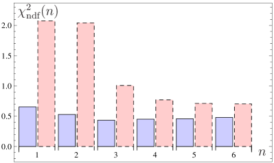
Figure 2: Dependence of the goodness of fit $\chi_{\text{ndf}}^{2}\equiv\chi^{2}/{\rm ndf}$ (ndf $=$ number of degrees of freedom) on the number $n$ of Gegenbauer harmonics shown as histograms: set-1—solid (blue) bars; set-2—higher dashed (red) bars.

The goodness of fit for set-1 is only slightly decreasing with $n$ and remains almost stable after $n=3$. Thus, 2 to 3 parameters are actually enough to describe all data in this region with $\chi_{\text{ndf}}^{2}\approx 0.5$. In contrast, the data description of set-2 is only possible with a $\chi_{\text{ndf}}^{2}$ value 2 or 3 times larger—even if we include more harmonics. To fit all the data, we are forced to consider at least 3 parameters with $\chi_{\text{ndf}}^{2}\approx 1$. To have an even better description with a goodness of fit approximately equal to 0.8, we have to employ 4 parameters. Further increase of the number $n$ will not provide any improvement.

However, for the sake of comparison of the results, one should use the same fit model of pion DA, which means that the most appropriate number of harmonics may be fixed to 3. Best-fit curves for both data sets are shown in Fig. 3 as a bunch of form-factor predictions with errors stemming from the sum of the statistical error and the twist-four uncertainties. At high values of the momentum transfer, the fit curve of the set-2 data—long dashed (red) line—exceeds the 68% CL (confidential level) region of the set-1 data fit—solid (blue) line. This indicates that in the framework of LCSRs, the new BaBar data above 9 GeV² deviate from the low-$Q^{2}$ data at the level of a 1$\sigma$ deviation and more.

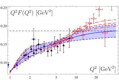
Figure 3: Best-fit curves to the experimental data for the transition form factor in the framework of LCSRs: solid (blue) line—best-fit curve of set-1; strip bounded by dashed (blue) lines—68% CL region; long dashed (red) line—best-fit curve of set-2; strip bounded by dashed dotted (red) lines—68% CL region. Error bars show the sum of the statistical errors and the twist-four uncertainties. The experimental data are taken from the CELLO CELLO91 (diamonds), CLEO CLEO98 (triangles), and BaBar BaBar09 (open crosses) experiments.

IV.2 Data analysis vs pion DA models

Performing the data analysis, we obtain the best-fit values of the pion DA in the 68% CL region for a number of harmonics $n=2\div 3$. The 3D graphics of the confidential regions for the 3 harmonics analysis were presented in our recent work in BMPS11 , whereas the best-fit values together with the statistical errors and the twist-four uncertainties are given in Table 1 below. We compare there our fit results with various pion DA models in terms of the goodness of fit $\chi_{\text{ndf}}^{2}$ for the two analyzed sets of experimental data. From the first two lines of Table 1, we infer that the inclusion of the new high-$Q^{2}$ BaBar data affect only the value of the parameter $a_{6}$, while $a_{2}$ and $a_{4}$ do not change significantly. Moreover, the good description of the experimental data up to 9 GeV² becomes appreciably worse after the inclusion of the high-$Q^{2}$ tail of the BaBar data. The BMS pion DA stands out in the sense that it provides the best fit for set-1, while all other models cannot reproduce these data good enough.

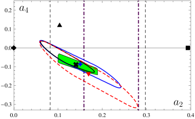
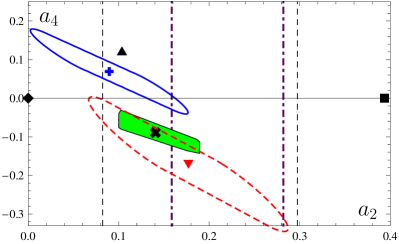
Figure 4: (color online). Distorted $1\sigma$ error ellipses for set-1 (upper panel) and set-2 (lower panel) from various experiments CELLO91 ; CLEO98 ; BaBar09 ; BaBar11-BMS using different data-analysis procedures. These ellipses result from merging together the ellipses associated with different values of the twist-four parameter in the range $\delta^{2}=0.15\div 0.23$ GeV². The slanted shaded (green) rectangle encloses the area of $a_{2}$ and $a_{4}$ values determined by NLC-SRs BMS01 , with the BMS pion DA being marked by ✖. The middle points of the ellipses (✚ and ▼), the asymptotic DA (◆), the CZ DA (◼), and Model III from ABOP10 (▲) are also marked. The range of values of $a_{2}$, restricted by lattice simulations, are indicated by vertical lines: Lat06 —dashed lines; Lat10 —dashed-dotted (blue) lines. All results are shown at the scale $\mu_{\text{SY}}^{2}=(2.4$ GeV$)^{2}$, whereas the treatment of the Borel parameter $M^{2}(Q^{2})$ is explained in the text. Graphics taken from BMPS11 .

It is worth remarking that one of the models, obtained from fitting the experimental data within the Modified Factorization Scheme (MFS), has the value $\chi_{\text{ndf}}^{2}=4.4$ in contrast to the result $\approx 1.1$ obtained in Kro10sud . This discrepancy indicates that using the same pion DA in the framework of LCSRs and the MFS may lead for the same observable to incompatible results—a theoretical bias.

Table 1: Measures of goodness of fit of selected pion DA models (first column) with associated coefficients $a_{n}$ (second column), used in the calculation of the pion-photon transition form factor by means of LCSRs. Note that the coefficients $a_{n}$ are strongly correlated and the errors of $a_{n}$ represent the maximal variation in the range of the $1\sigma$-region. The last two columns show the values of $\chi_{\text{ndf}}^{2}$ for the data in set-1 and for the whole set of the data, (set-2), respectively. All values of the coefficients $a_{n}$ are given at the scale $\mu_{\text{SY}}=2.4$ GeV SY99 .

Model/Fit $(a_{2},a_{4},\ldots)_{\mu^{2}=\mu_{\text{SY}}^{2}}$ $\chi^{2}_{\text{ndf}},~{}[1-9]$ GeV² $\chi^{2}_{\text{ndf}},~{}[1-40]$ GeV² 3D fit, $[1-9]$ GeV² $(0.17\pm 0.11,-0.14\pm 0.18,0.12\pm 0.17)$ $0.4$ $-$ 3D fit, $[1-40]$ GeV² $(0.18\pm 0.11,-0.17\pm 0.17,0.31\pm 0.12)$ $-$ $1.0$ NLC-SRs, BMS BMS01 $(0.141,-0.089)$ $0.5$ $3.1$ Model I ABOP10 $(0.084,0.137,0.088)$ $\geq 2.8$ $\geq 2.4$ Modif. fact. Kro10sud $(0.21,0.009)$ $3.8$ $4.4$ AdS/QCD, BT07 $(0.15,0.06,0.03,\ldots)$ $2.3$ $2.8$ CZ CZ84 $(0.394,0)$ $32.3$ $25.5$ Asympt. $(0,0)$ $4.7$ $7.9$

Below, we consider in detail the results of the 2D analysis in the $(a_{2},a_{4})$ plane, presented in Fig. 4, with the upper panel showing the results for set-1, whereas the lower panel presents those for set-2. To this end, we calculate the $1\sigma$ error ellipses by allowing the parameter $\delta^{2}$ to vary by $20\%$ around the value 0.19 GeV². The obtained error ellipses are then unified into a single (distorted) $1\sigma$ ellipse shown in Fig. 4. To be specific, we consider the following cases: (i) The result of combining the projections on the plane $(a_{2},a_{4})$ of the 3D (3 parameter) data analysis is represented by the largest ellipse—dashed (red) line with the middle point ▼. (ii) The analogous result of the 2D (2 parameter) data analysis in terms of $a_{2}$ and $a_{4}$ is shown by the smaller ellipse (solid blue line) with the middle point ✚ having the coordinates $(0.15,-0.09)$ and $\chi^{2}_{\text{ndf}}\approx 0.5$, that almost coincides with the middle point ✖ of the parameter area determined by NLC-SRs BMS01 . (iii) The combination of the intersections with the $(a_{2},a_{4})$ plane of all 3D ellipsoids generated by the variation around the central value of $\delta^{2}$ give rise to the smallest ellipse (thick line), entirely enclosed by the previous one.

For convenience, the locations in the $(a_{2},a_{4})$ plane of some characteristic pion DAs are also indicated in Fig. 4. These are the asymptotic DA (◆), the CZ model (◼), and the projection of Model III from ABOP10 (▲). Note that the slanted (green) rectangle, containing those values of $a_{2}$ and $a_{4}$ that have been determined by NLC-SRs BMS01 , is practically within both larger error ellipses and also overlapping with the smallest one. Moreover, the BMS model DA ✖ stands out by lying inside of all $1\sigma$ error ellipses. Thus, the theoretical predictions obtained from the 2D and the 3D data analyses conform with each other and agree at the level of $\chi^{2}_{\text{ndf}}\leq 0.5$ with the results obtained from NLC-SRs BMS01 . The calculated $1\sigma$ error ellipses comply rather good with the boundaries for $a_{2}$ extracted from two independent lattice simulations. The vertical dashed lines denote in both panels the older estimate from Lat06 , while the very recent constraints from Ref. Lat10 are represented by the dashed-dotted (blue) vertical lines.

From the lower panel of Fig. 4 it becomes evident that the situation changes significantly when including in the analysis the high-$Q^{2}$ tail of the BaBar data BaBar09 . Indeed, using the same designations as in the upper panel, we display the analogous unified error ellipses and observe that the error ellipsoid has no intersection with the $(a_{2},a_{4})$ plane, whereas the composed error ellipse resulting from the 2D analysis (solid blue line) deviates from the region of negative values of $a_{4}$ and moves inside its positive domain. At the same time, the fit quality deteriorates yielding $\chi^{2}_{\text{ndf}}\approx 2$, as opposed to the value $\chi^{2}_{\text{ndf}}\approx 0.5$ determined for set-1 of the data. As regards the unified $1\sigma$ error ellipse of the 3D projections on the $(a_{2},a_{4})$ plane (larger dashed red ellipse), its position remains unaffected, still enclosing most of the area of the $a_{2}$, $a_{4}$ values computed with NLC-SRs—shaded (green) rectangle.

     

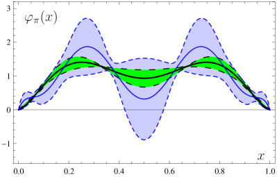
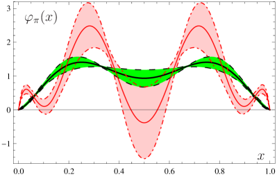
Figure 5: Left. Comparison of the BMS pion DA bunch (shaded strip in green color) and of the BMS model (black solid line inside this strip) with the 3D fit to the experimental data on the pion-photon transition form factor. The solid blue line denotes the best-fit pion DA sample obtained from the analysis of set-1, with the dashed lines indicating the sum of the statistical errors of the fit and the twist-four uncertainties. Right. Analogous results obtained with set-2.

The high quality of the data fit parallels the lattice findings, with the 3D error ellipse being almost entirely inside the boundaries from Lat06 (dashed vertical lines), while it also overlaps for the larger values of $a_{2}$ with the range of values computed in Lat10 (dashed-dotted vertical lines). In contrast, the ellipse from the 2D analysis agrees very roughly with the small $a_{2}$ window of Lat10 , sharing also only a small common area with the low end of the $a_{2}$ region found in Lat06 . Obviously, no agreement between the 2D and the 3D analysis is found. This discrepancy is also reflected in the values of the $\chi$-criterion of the 2D fit model $\chi^{2}_{\text{ndf}}\approx 2$ and that for the 3D model which turns out smaller by a factor of 2: $\chi^{2}_{\text{ndf}}\approx 1$. This means that a pion DA, based only on 2 harmonics, is not sufficient to describe all the data on the pion-photon transition form factor. This deviating behavior of the results, associated with the fits for set-1 and set-2, shows up for a larger number of degrees of freedom, i.e., when including into the data analysis the next higher harmonics $\psi_{n}$ with $n=6,8,10$. But, for the case of the set-1 fit, this expansion does not improve any further the value $\chi^{2}_{\text{ndf}}\leq 0.5$—this remains approximately stable. Moreover, the $1\sigma$-admissible regions in 2D, 3D, or 4D parameterizations appear to be each embedded inside the other. In contrast, fitting the set-2 data, these new degrees of freedom lead to a decrease of $\chi^{2}_{\text{ndf}}$, while the corresponding $1\sigma$-regions in the 2D, 3D, or 4D space, either do not overlap at all or intersect only marginally.

It becomes obvious from Fig. 4 that Model III (▲) from ABOP10 has a projection on the $(a_{2},a_{4})$ plane that lies outside of all considered $1\sigma$ error ellipses of the data. However, selecting for the Borel parameter the value $M^{2}=1.5$ GeV², as in ABOP10 , the agreement of this model with the data improves to the level of $\chi^{2}_{\text{ndf}}\gtrsim 1.5$.

IV.3 Pion DA characteristics

The confidential region of the coefficients $\{a_{n}\}$, obtained above, can be linked to any other characteristic of pion DA. The profiles of the pion DA $\varphi_{\pi}(x)$, extracted in the 3D fit procedure, are shown in Fig. 5: left panel—set-1; right panel—set-2. The BMS bunch (shaded green strip) and the BMS DA model (black solid line) are also shown in both cases. The inclusion into the data fit of the high-$Q^{2}$ BaBar tail, causes a modification of the shape of the pion DA—see Fig. 5—giving support to our previous observation that the BMS bunch is within the error range of the set-1 fit (left panel), while the best fit to set-2 differs considerably (right panel). In addition, the pion DA becomes endpoint enhanced, as opposed to the endpoint-suppressed BMS pion DA. The endpoint behavior can be characterized by its slope at the origin given by the derivative $\varphi_{\pi}^{\prime}(0)$ or, more adequately, by the so-called “integral derivative” $D^{(2)}\varphi_{\pi}(x)$, introduced in MPS10 . The integral derivative is the average derivative $\varphi^{\prime}_{\pi}(x)$ defined by

$$D^{(2)}\varphi(x)=\frac{1}{x}\int_{0}^{x}\frac{\varphi(y)}{y}dy$$

with the important property $\lim\limits_{x\to 0}D^{(2)}\varphi(x)=\varphi^{\prime}_{\pi}(0).$

Table 2: Comparison of the pion DA characteristics for the data of set-1 and set-2.

data set $[1-9]$ GeV² $[1-40]$ GeV² $\varphi^{\prime}_{\pi}(0)$ $20.2\pm 19.8\pm 1.1$ $48.5\pm 11.4\pm 0.4$ $D^{(2)}\varphi_{\pi}(0.4)$ $6.6\pm 1.1\pm 0.4$ $8.1\pm 0.7\pm 0.3$ BMS DA Agreement No $n$ 2, 3 3, 4 $\chi^{2}_{\text{ndf}}$ 0.53,    0.44 $1.0,\,\,\,0.77$

Using a 3D confidential bound on the Gegenbauer coefficients, we get the values of the derivatives $\varphi^{\prime}_{\pi}(0)$ and $D^{(2)}\varphi(0.4)$, supplied in Table 2 for both data sets. These characteristics are shown together with the theoretical errors, the first being statistical and the second stemming from the twist-four uncertainty. We observe that these characteristics can clearly differentiate the pion DAs generated from set-1 and set-2.

IV.4 Combining Lattice constraints with experimental data

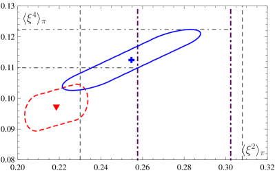
Figure 6: (color online). Predictions for the moments $\langle\xi^{2}\rangle_{\pi}$ and $\langle\xi^{4}\rangle_{\pi}$ at the lattice scale $\mu^{2}_{\text{Lat}}=4$ GeV². The solid (blue) ellipse corresponds to our choice of $M^{2}$, whereas the dashed (red) one results when using $M^{2}=1.5$ GeV². The vertical lines show the range of values computed on the lattice: dashed line—Lat06 ; dashed-dotted (violet) line—Lat10 .

The possibility to extract information on the moment $\langle\xi^{4}\rangle_{\pi}$ of the pion DA by combining lattice constraints with the experimental data was first pointed out in Ste08 and the following range of values was extracted from the $1\sigma$ error ellipse of the CLEO data CLEO98 in conjunction with the lattice constraints for $\langle\xi^{2}\rangle_{\pi}$ from Lat07 : $\langle\xi^{4}\rangle_{\pi}\in[0.095\div 0.134]$ at $\mu^{2}_{\text{Lat}}=4$ GeV² and for $M^{2}=0.7$ GeV². This procedure was refined in BMPS11 in the following way: first, we expanded the result of the 2D analysis to the $(\langle\xi^{2}\rangle_{\pi},\langle\xi^{4}\rangle_{\pi})$ moments. Then, we determined the intersection of the confidential region (the area enclosed by a solid blue line) in Fig. 6 for set-1 (cf. Fig. 4) using the constraints from Lat06 and Lat10 . The intersection of these constraints, evaluated at the typical lattice scale $\mu^{2}_{\text{Lat}}=4$ GeV², and the experimental data leads to the following moment results, respectively, (i) $\langle\xi^{2}\rangle_{\pi}\in[0.23\div 0.29]$ and $\langle\xi^{4}\rangle_{\pi}\in[0.102\div 0.122]$, (ii) $\langle\xi^{2}\rangle_{\pi}\in[0.26\div 0.29]$ and $\langle\xi^{4}\rangle_{\pi}\in[0.11\div 0.122]$. These common validity ranges were extracted using a $Q^{2}$-dependent Borel parameter—like everywhere in our analysis here and in BMPS11 . On the other hand, the value $M^{2}=1.5$ GeV² ABOP10 , yields only a small intersection of the validity region extracted from set-1 (shown in Fig. 6 by the dashed red line) with the lattice constraints of Lat06 . This restricts the common region of validity to the value $\langle\xi^{4}\rangle_{\pi}\simeq 0.1$, whereas there is no intersection at all with the lattice estimates from Lat10 . This obvious sensitivity of $\langle\xi^{2}\rangle_{\pi}$ on the choice of the particular value of the Borel parameter $M^{2}$ gives additional support to our choice of the value of the Borel parameter.

V Conclusions

We have presented here a global fit to the data on the pion-photon transition form factor, discussing further our recent analysis in BMPS11 . To get a precise measure of the influence of the high $Q^{2}$ BaBar data on the form factor and the pion DA, we divided the experimental data in two different sets with respect to $Q^{2}$. Set 1 contains all data in the range $[1\div 9]$ GeV², whereas the second set comprises all data in the regime covered by BaBar, i.e., $[1\div 40]$ GeV². As a result, we obtained the confidential regions of different characteristics of the pion DA (Gegenbauer coefficients, derivatives of $\varphi_{\pi}(x)$ at $x=0$, and its moments) by fitting the experimental data within the framework of LCSRs. The predictions obtained from the CELLO, CLEO, and the BaBar data up to 9 GeV² are in good agreement with the previous fits, based only the CLEO data SY99 ; BMS02 ; BMS03 ; BMS05lat ; MS09 , giving preference to an endpoint-suppressed pion DA BMS01 . Beyond 9 GeV², the best fit requires a sizeable coefficient $a_{6}$ that inevitably leads to an endpoint-enhanced pion DA. The data analysis tells us that the inclusion of the high-$Q^{2}$ tail of the BaBar data affects mainly the Gegenbauer coefficient $a_{6}$, while $a_{2}$ and $a_{4}$ change only insignificantly. The good description of the experimental data up to 9 GeV² using LCSRs becomes considerably less accurate after the inclusion of the high-$Q^{2}$ data but yields an acceptable value of $\chi^{2}_{\text{ndf}}\approx 1$. This effect has been discussed before in MS09Trento at a qualitative level. The results obtained with the inclusion of the high-$Q^{2}$ tail of the BaBar data indicate a possible discrepancy between the result of the BaBar experiment and the method of LCSRs. Indeed, the high-$Q^{2}$ BaBar data require a pion DA with a sizeable number of higher Gegenbauer coefficients $a_{n}$, or alternative theoretical schemes outside the standard QCD factorization approach, see, e.g., Rad09 ; Pol09 ; Dor09 ; KOT10plb ; SZ11 ; WH10 . Similar conclusions were also drawn in RRBGGT10 using Dyson–Schwinger equations and in the recent works BCT11 , based on AdS/QCD.

VI Acknowledgments

We would like to thank Simon Eidelman, Andrei Kataev, and Dmitri Naumov for stimulating discussions and useful remarks. A. P. wishes to thank the Ministry of Education and Science of the Russian Federation (“Development of Scientific Potential in Higher Schools” projects No. 2.2.1.1/12360 and No. 2.1.1/10683). This work was supported in part by the Heisenberg–Landau Program under Grant 2011, the Russian Foundation for Fundamental Research (Grant No. 11-01-00182), and the BRFBR–JINR Cooperation Program under contract No. F10D-002.

References

- (1) S.J. Brodsky, G.P. Lepage, Adv. Ser. Direct. High Energy Phys. 5 (1989) 93.
- (2) A.V. Efremov, A.V. Radyushkin, Phys. Lett. B 94 (1980) 245. G.P. Lepage, S.J. Brodsky, Phys. Rev. D 22 (1980) 2157.
- (3) F. del Aguila, M.K. Chase, Nucl. Phys. B 193 (1981) 517; E. Braaten, Phys. Rev. D 28 (1983) 524. E.P. Kadantseva, S.V. Mikhailov, A.V. Radyushkin, Sov. J. Nucl. Phys. 44 (1986) 326.
- (4) B. Melić, D. Müller, K. Passek-Kumerički, Phys. Rev. D 68 (2003) 014013.
- (5) A.V. Radyushkin, Dubna preprint P2-10717, 1977 [hep-ph/0410276].
- (6) V.L. Chernyak, A.R. Zhitnitsky, Phys. Rept. 112 (1984) 173.
- (7) A.P. Bakulev, S.V. Mikhailov, N.G. Stefanis, Phys. Lett. B 508 (2001) 279; Erratum: ibid. B590, 309 (2006).
- (8) H.J. Behrend et al., Z. Phys. C 49 (1991) 401.
- (9) J. Gronberg et al., Phys. Rev. D 57 (1998) 33.
- (10) B. Aubert et al., Phys. Rev. D 80 (2009) 052002.
- (11) A. Khodjamirian, Eur. Phys. J. C 6 (1999) 477.
- (12) K. Nakamura et al., J. Phys. G 37 (2010) 075021.
- (13) A.P. Bakulev, S.V. Mikhailov, A.V. Pimikov, N.G. Stefanis, Phys. Rev. D 84 (2011) 034014.
- (14) S.V. Mikhailov, N.G. Stefanis, Nucl. Phys. B 821 (2009) 291; corrected in arXiv:0905.4004v6.
- (15) S.S. Agaev, V.M. Braun, N. Offen, F.A. Porkert, Phys. Rev. D 83 (2011) 054020.
- (16) A.P. Bakulev, S.V. Mikhailov, N.G. Stefanis, Phys. Rev. D 67 (2003) 074012.
- (17) A.P. Bakulev, S.V. Mikhailov, N.G. Stefanis, Phys. Lett. B 578 (2004) 91.
- (18) A.P. Bakulev, S.V. Mikhailov, N.G. Stefanis, Phys. Rev. D 73 (2006) 056002.
- (19) V.M. Braun, I.E. Filyanov, Z. Phys. C 44 (1989) 157.
- (20) S.S. Agaev, Phys. Rev. D 72 (2005) 114010.
- (21) P.d. A. Sanchez, it et al., 1101.1142.
- (22) V.M. Braun et al., Phys. Rev. D 74 (2006) 074501.
- (23) R. Arthur et al., Phys. Rev. D 83 (2011) 074505.
- (24) P. Kroll, Eur. Phys. J. C 71 (2011) 1623.
- (25) A. Schmedding, O. Yakovlev, Phys. Rev. D 62 (2000) 116002.
- (26) S.J. Brodsky, G.F. de Teramond, Phys. Rev. D 77 (2008) 056007.
- (27) S.V. Mikhailov, A.V. Pimikov, N.G. Stefanis, Phys. Rev. D 82 (2010) 054020.
- (28) N.G. Stefanis, Nucl. Phys. Proc. Suppl. 181–182 (2008) 199.
- (29) M.A. Donnellan et al., PoS LAT2007 (2007) 369.
- (30) S. V. Mikhailov and N. G. Stefanis, Mod. Phys. Lett. A24, 2858 (2009).
- (31) A.V. Radyushkin, Phys. Rev. D 80 (2009) 094009.
- (32) M.V. Polyakov, JETP Lett. 90 (2009) 228.
- (33) A.E. Dorokhov, Phys. Part. Nucl. Lett. 7 (2010) 229.
- (34) Y.N. Klopot, A.G. Oganesian, O.V. Teryaev, Phys. Lett. B 695 (2011) 130.
- (35) A. Stoffers, I. Zahed, arXiv:1104.2081.
- (36) X.-G. Wu and T. Huang, Phys. Rev. D82, 034024 (2010); arXiv:1106.4365 [hep-ph].
- (37) H.L.L. Roberts et al. Phys. Rev. C 82 (2010) 065202.
- (38) S.J. Brodsky, F.-G. Cao, G.F. de Teramond, Phys. Rev. D 84 (2011) 033001; arXiv:1105.3999.