Emergence of robustness against noise: A structural phase transition in evolved models of gene regulatory networks

Abstract

We investigate the evolution of Boolean networks subject to a selective pressure which favors robustness against noise, as a model of evolved genetic regulatory systems. By mapping the evolutionary process into a statistical ensemble and minimizing its associated free energy, we find the structural properties which emerge as the selective pressure is increased and identify a phase transition from a random topology to a “segregated core” structure, where a smaller and more densely connected subset of the nodes is responsible for most of the regulation in the network. This segregated structure is very similar qualitatively to what is found in gene regulatory networks, where only a much smaller subset of genes — those responsible for transcription factors — is responsible for global regulation. We obtain the full phase diagram of the evolutionary process as a function of selective pressure and the average number of inputs per node. We compare the theoretical predictions with Monte Carlo simulations of evolved networks and with empirical data for Saccharomyces cerevisiae and Escherichia coli.

I Introduction

Many large-scale dynamical systems are composed of elementary units which are noisy, i.e., can behave non-deterministically, but nevertheless must behave globally with some degree of predictability. A paradigmatic example is gene regulation in the cell, which is a system of many interacting agents — genes, mRNA, and proteins — which are subject to stochastic fluctuations. What makes gene regulation particularly interesting is that it is assumed to be under evolutionary pressure to preserve its dynamic memory against stochastic fluctuations Kitano (2004); Raser and O’Shea (2005); Maheshri and O’Shea (2007). Many important cellular processes require such reliability, such as circadian oscillations Raser and O’Shea (2005). Furthermore, in multicellular organisms, errors in signal transduction can potentially lead to catastrophic consequences, such as embryo defects or cancer Kitano (2004); Gutkind (2000). Since the source of noise cannot be fully removed Lestas et al. (2010), a gene regulation system must adopt characteristics which compensate for the unavoidably noisy nature of its elements. Since they are a product of natural selection, these characteristics must emerge from random mutations and subsequent selection based on fitness. A central question concerns the general large-scale features which are likely to emerge in this scenario that result in reliable function under noise. In this work, we study the emergence of robustness against noise in networks of Boolean elements which are subject to selective pressure, functioning as a model for evolved gene regulatory systems. We show that the system undergoes a structural phase transition at a critical value of selective pressure, from a totally random topology to a “segregated-core” structure, where a smaller and more densely connected subset of the network is responsible for the regulation of most nodes in the network. This characteristic is present to a significant degree in gene regulatory systems of organisms such as yeast and Escherichia coli, in which all the regulation is done by a much smaller (and denser) subset of the network, comprised of transcription factor genes.

Boolean networks (BNs) have been used extensively to model gene regulation Kauffman (1969a, b); Bornholdt (2005); Drossel (2008). The Boolean value on a given node represents the level of concentration of proteins encoded by a gene, which in the simplest approximation can be either “on” or “off.” The regulation of genes by other genes is represented by Boolean functions associated with each node, which depend on the state of other nodes called the inputs of the function. The dynamics on these networks serve as a model for the mutual regulation of genes which control the metabolism of cells in an organism. Gene regulation is composed of specific steps involving the production of proteins and other metabolites, which need to be carried out in specific sequences and under certain conditions. During each of these steps the dynamics is subject to stochastic fluctuations Raser and O’Shea (2005); Maheshri and O’Shea (2007); Raj and van Oudenaarden (2008), since the number of proteins involved can be very low Raser and O’Shea (2005); Eldar and Elowitz (2010), and the whole process lacks an inherent synchronization mechanism. In order for the regulation process to work reliably, the network must possess some degree of robustness against these perturbations Kollmann et al. (2005). Indeed, the investigation of real regulatory networks modelled as BNs, such as the one responsible for the yeast cell cycle Li et al. (2004), revealed a remarkable degree of robustness, where most trajectories in state space lead to the same attractor, regardless of the initial conditions. Similar results were also obtained for the segment polarity regulatory network in Drosophila melanogaster Albert and Othmer (2003); Chaves et al. (2005), which showed that wild-type attractors are significantly robust to different initial conditions and perturbations, and seem to depend only on general topological characteristics of the network, instead of specific functional details. However, the general features which make BNs robust against different types of perturbations are still being identified.

Perhaps the simplest form of perturbation one can consider is a “flip” of a single node in the network, and the propagation of flips which result from it. This corresponds to the situation where the stochastic noise is very weak, and can be modeled as a single flip event. After the perturbation, the system has an arbitrary amount of time to recover (if it recovers), and different perturbations do not build up. Many authors have considered the robustness against perturbations of this type, including Kauffmann Kauffman (1969a, b) who was the first to propose random Boolean networks (RBNs) — networks with fully random topology and functions — as a model of gene regulation. According to this type of perturbation, the dynamics of RBNs Drossel (2008) can belong to one of two phases, depending on the number of inputs per node $K$: A frozen phase ($K<2$) where the perturbation propagates sub-linearly in time and eventually dies out; and a “chaotic” phase ($K>2$) where the perturbation grows exponentially and eventually reaches the entire system. A critical line exists at $K=2$, where the perturbation grows algebraically, and features from both phases are simultaneously observed.

Although RBNs in the frozen phase and on the critical line show features which can be interpreted as robustness in some sense, they fall short of being convincing models for gene regulation. Actual gene regulation networks are not random and show a high degree of topological Maslov and Sneppen (2005) and functional Harris et al. (2002) organization which are not present in simple RBNs. Conceivably, these features arise out of stringent requirements to perform specific tasks and of types of robustness which are more demanding than the containment of single flip perturbations. As an attempt at producing more complete models, many authors investigated the evolution of BN systems, where the fitness criterion is some form of robustness against perturbation which is not inherent to RBNs. The majority of authors assumed single flips as the only type of noise, but considered different types of responses as fitness criteria Bornholdt and Sneppen (1998, 2000); Stern (1999); Bassler et al. (2004); Aldana et al. (2007); Szejka and Drossel (2007); Mihaljev and Drossel (2009); Pomerance et al. (2009), most of which are related to the capacity of the network to display the same dynamical pattern after a single-flip. In particular, in Szejka and Drossel (2007) it was found that if the fitness criterion is the ability to return to the same attractor after the perturbation, the evolved networks always achieve maximum fitness. Furthermore these networks with maximum fitness span a huge portion of configuration space, and show a high degree of variability. This means not only that this type of robustness can evolve, but also that it is not a very demanding task for the evolutionary process.

In this work, we consider the arguably more realistic situation where the perturbations are caused by transcriptional noise, which can be arbitrarily frequent . In this scenario, the effects of noise can overlap and build up in time. The appropriate fitness criterion remains whether or not the network is capable of performing some predefined dynamical pattern, but this is a task which becomes much more complicated. In fact, it can be shown that for networks which are sparse, i.e., the average number of inputs per node is some finite number, perfect robustness can never be achieved, and some amount of deviations, or “errors,” in the dynamics are always going to exist Peixoto (2010, 2012). Instead, one measures robustness not only by the amount of existing errors, but also by the ability of the system to not be overtaken by them and consequently lose all memory of its dynamical past — i.e., to become ergodic. This type of robustness is much stronger than, and not necessarily related to the ability of the system to contain single-flip perturbations. This was shown in Peixoto and Drossel (2009a) for RBNs subject to transcriptional noise, for which neither phase (chaotic or frozen) is robust, and both display ergodic behavior, for any non-zero value of noise.

Furthermore, unlike Bornholdt and Sneppen (1998, 2000); Stern (1999); Bassler et al. (2004); Szejka and Drossel (2007); Mihaljev and Drossel (2009), in this work we also consider the cost which is associated with different levels of robustness. It is generally the case that improved robustness can be obtained by introducing redundancy or some other mechanism that counteracts the effect of noise, which increases the overhead in the system. This added overhead can impact negatively on the fitness of the organism, which needs to spend more energy or more time to perform the same task. Therefore the trade-off between overhead and robustness is also driven by the evolutionary process. In this work, this overhead is controlled by fixing the average in-degree during the evolutionary process, which becomes an external parameter. By selecting the appropriate value, one automatically determines a selective pressure that yields the corresponding trade-off.

Our main result is that under transcriptional noise, the selective pressure can have a very noticeable effect on large-scale properties of the system: If it is large enough, it triggers a structural phase transition, where networks change from a random topology to a segregated-core structure, with most nodes being regulated by a smaller and denser subset of the network. This observed segregated-core topology is strikingly similar (even if qualitatively so) to what is observed in most real gene regulation networks; namely, genes are separated into two classes: target genes, and those which regulate transcription factors. Only transcription factor genes are responsible for regulation of other genes, and they are usually orders of magnitude smaller in number than target genes Nimwegen (2006).

This work is divided as follows. We begin in Sec. II by presenting the model, and in Sec. III we define the evolutionary process and map it into an equivalent Gibbs ensemble. We then parametrize the topological characteristics of the system as a stochastic blockmodel in Sec. IV, and obtain an expression for its entropy. In Sec. V we describe the technique used to minimize the free energy. We follow in Sec. VI with the characterization of the existing phase transition and obtain the phase diagram. We perform comparisons with Monte Carlo simulations in Sec. VII and with the gene regulatory networks of yeast and E. coli in Sec. VIII. Finally, we conclude with a discussion.

II The model

A Boolean network Kauffman (1969a); Drossel (2008) is a directed graph of $N$ nodes representing Boolean variables $\mathbf{\sigma}\in\{1,0\}^{N}$, which are subject to a deterministic update rule,

$$\sigma_{i}(t+1)=f_{i}\left(\bm{\sigma}(t)\right)$$ (1)

where $f_{i}$ is the update function assigned to node $i$, which depends exclusively on the states of its inputs. At a given time step all nodes are updated in parallel.

We include noise in the model by introducing the probability $P$ that at each time step a given input has its value “flipped”: $\sigma_{j}\to 1-\sigma_{j}$, before the output is computed Peixoto and Drossel (2009a). This probability is independent for all inputs in the network, and many values may be flipped simultaneously. The functions on all nodes are taken to be the majority function, defined as

$$f_{i}(\{\sigma_{j}\})=\begin{cases}1\text{ if }\sum_{j}\sigma_{j}>k_{i}/2,\\ 0\text{ otherwise, }\end{cases}$$ (2)

where $k_{i}$ is the number of inputs of node $i$. It is assumed throughout the paper that the values of $k_{i}$ are always odd . This is so chosen because odd-valued majority functions are optimal, since no other function performs better against noise Evans and Schulman (2003). By using Eq. 2, we essentially remove the choice of functions from the evolutionary process and concentrate solely on topological aspects.

Starting from an initial configuration, the dynamics of the system evolves and eventually reaches a dynamically stable regime, where the average fraction $b_{t}$ of nodes with value $1$ no longer changes, except for stochastic fluctuations which vanish for a large system size Huepe and Aldana-González (2002); Peixoto (2012). In the absence of noise ($P=0$) there are only two possible attractors (if the network is sufficiently well connected) where all nodes have the same value, which can be either $0$ or $1$. We will consider these homogeneous attractors as representing the “correct” dynamics, and denote the deviations from them as “errors.” More specifically, and without loss of generality, we will name the value of $1$ as an “error,” and the value of $b_{t}$ as the average error on the system.

The steady-state fraction of errors $b^{*}\equiv\lim_{t\to\infty}b_{t}$ (for $b_{0}=0$) will increase with $P$. For any network with a finite average in-degree there will be a critical value of noise $P^{*}$ for which the dynamics undergoes a phase transition, and the value of $b^{*}$ reaches $1/2$, and remains at this value for $P>P^{*}$ Peixoto (2010). The value $b^{*}=1/2$ is special, since it means that the dynamics lost the memory of its initial state, since any other initial value of $b_{0}$ (including $b_{0}>1/2$) would lead eventually to this same value of $b^{*}$. Therefore, the value of $P^{*}$ marks the transition from a nonergodic to an ergodic dynamics. Robustness against noise is synonymous with nonergodicity, since only in this regime are dynamical correlations not destroyed over time.

BNs with majority functions serve as a paradigmatic model for networks robust against noise, since they are composed of optimal elements, and they show a minimal dynamical behavior in the absence of noise, namely two homogeneous attractors with $\{\sigma_{i}\}=0$ or $1$. If robustness cannot be attained for such a system, it is much less likely to be possible for a different system with a another choice of Boolean functions, or displaying a more elaborate dynamical pattern Peixoto (2012).

In this work we will consider the value of the steady-state average error $b^{*}$ as the main fitness criterion governing the survival probability of an organism, since it directly measures the deviation from the situation without noise. Although the phenotype itself, i.e. the dynamics without noise, does not change during the evolutionary process considered here, its stability, as measured by $b^{*}$, does. This translates into an actual fitness criterion, since it is not enough for phenotypes to exist; they must also be stable against perturbations. If they are not, they are not viable in practice, and thus should not be observed.

III Evolutionary dynamics

We suppose that a given BN represents the genotype of a full organism, which can self-replicate and belongs to a population that is subject to an evolutionary pressure. The number of individuals in the population is assumed to be sufficiently large and constant. Individuals replicate a given number of times with a constant rate. Parents die the moment they replicate. The offspring are always initially identical to their parents, but are individually subject to point mutations represented by the matrix $\mu_{ij}$, which defines the probability of mutating from genotype (i.e. network) $i$ to $j$. The offspring survive with probability $a_{i}$, given by the Boltzmann selection criterion

$$a_{i}\propto e^{\beta f_{i}},$$ (3)

where $f_{i}$ is the fitness of genotype $i$. The parameter $\beta$ controls the selective pressure: For large values of $\beta$ only the very best networks survive, whereas for smaller values most networks do. As mentioned previously, the fitness of a network will be given by the fraction of ones (“errors”) after a sufficiently long time, $b^{*}_{(i)}\equiv\lim_{t\to\infty}b_{t}^{(i)}$, for $b_{0}^{(i)}=0$, as

$$f_{i}=-Nb^{*}_{(i)}.$$ (4)

Thus, the largest fitness a network can have is $f_{i}=0$, which should be possible only if there is no noise ($P=0$).

We suppose that the global offspring mortality rate is such that the size of the population always remains constant. If we consider that the dynamics occurs in discrete time steps, we can write the probability $\pi_{i}(t)$ of finding an individual in the population with genotype $i$ at time $t$ as a Markov chain,

$$\pi_{i}(t)=a_{i}\sum_{j}\pi_{j}(t-1)\mu_{ji}.$$ (5)

The mutation probabilities $\mu_{ji}$ have a decisive effect on what topologies emerge. Mutations in actual biological systems may result in topological bias, such as gene duplications, which are not reversible and result in networks with broad degree distributions Ispolatov et al. (2005); Enemark and Sneppen (2007). However, the central aim here it to obtain the most likely topology that arises due to the selective pressure alone. For this reason we are more interested in mutations which will lead to all possible networks with equal probability in the absence of selective pressure (i.e. ergodicity). A simple and conventional choice is reversible mutations, $\mu_{ij}=\mu_{ji}$, for which the steady state $\pi_{i}\equiv\lim_{t\to\infty}\pi_{i}(t)$ obeys the detailed balance condition: $\pi_{i}\mu_{ij}a_{j}=\pi_{j}\mu_{ji}a_{i}$. This is a sufficient condition for the desired ergodicity property, but it is not strictly necessary, since other types of mutations may also fulfill it. However, from this condition we easily obtain that the steady-state probability of finding an individual with genotype $i$ is given by its survival probability,

$$\pi_{i}=a_{i}=e^{\beta f_{i}}/\mathcal{Z},$$ (6)

where $\mathcal{Z}=\sum_{i}e^{\beta f_{i}}=\sum_{i}e^{-\beta Nb^{*}_{(i)}}$. This corresponds exactly to a Gibbs ensemble of all possible genotypes, with a partition function given by $\mathcal{Z}$, where $Nb^{*}_{(i)}$ plays the role of the “microstate energy” and $\beta$ is the “inverse temperature” (these are of course only mathematical analogies, since these quantities do not actually represent a physical energy and temperature, respectively). The average intensive “energy” in the ensemble is thus

$$b^{*}=\sum_{i}b^{*}_{(i)}e^{-\beta Nb^{*}_{(i)}}/\mathcal{Z},$$ (7)

and the canonical entropy is

$$\mathcal{S}=-\sum_{i}\pi_{i}\ln\pi_{i}=\ln\mathcal{Z}+\beta Nb^{*}.$$ (8)

The objective is to obtain not only $b^{*}$ for a given $\beta$, but also the network topologies which characterize the ensemble. Instead of considering all microstates individually (i.e., all possible networks) and computing Eqs. 7 and 8 directly, we may parametrize the whole ensemble via some macroscopic variables $\{x_{j}\}$ which sufficiently describe its topological properties. These variables must be chosen so that it is possible to write both $b^{*}(\{x_{j}\})$ and $\mathcal{S}(\{x_{j}\})$ as functions of these variables alone. The entropy can, for instance, be obtained via the microcanonical formulation

$$\mathcal{S}(\{x_{j}\})=\ln\Omega(\{x_{j}\}),$$ (9)

where $\Omega(\{x_{j}\})$ is the number of different networks given a macroscopic parametrization $\{x_{j}\}$. The values of $\{x_{j}\}$ which correspond to thermodynamic equilibrium [i.e., the steady state of Eq. 5] can be obtained by minimizing the “free energy”,

$$\mathcal{F}(\{x_{j}\})=Nb^{*}(\{x_{j}\})-\mathcal{S}(\{x_{j}\})/\beta,$$ (10)

with respect to $\{x_{j}\}$. This stems from the principles of maximum entropy and minimum energy, for closed systems with fixed energy and entropy, respectively, which need to hold in thermodynamic equilibrium Callen (1985). It should again be emphasized that the theory so far is only a mathematical tool, which, although exact, says nothing about the actual physical thermodynamical properties of the evolved systems, i.e., they have no relation to an actual measurable energy or temperature. Instead, the minimization of Eq. 10 is entirely analogous to obtaining the steady state of Eq. 5 by any other means. However, this approach, together with an appropriate topological parametrization, allows us to obtain the outcome of the evolutionary process on the population, without having to actually implement any dynamics. As will be described in detail in the next section, we will parametrize the ensemble as a general stochastic blockmodel, which allows for a wide range of topological configurations, while at the same time allowing for a tractable computation of $b^{*}$ and $S$, which then can be used to minimize $\mathcal{F}$.

It should also be mentioned at this point that we are interested in the properties of typical networks in the ensemble when the selective pressure $\beta$ is varied, under the restriction that the average number of inputs per node (the average in-degree) ${\left<k\right>}$ is always the same. As mentioned in the introduction, this restriction originates from the assumption that a larger number of inputs increases the putative cost for the organism of realizing a regulatory mechanism which depends on more elements. Thus, the value of ${\left<k\right>}$ should on its own impact the fitness of the organism, and should also be subject to natural selection. For simplicity, we do not describe the fitness landscape which depends on ${\left<k\right>}$ and its evolution, in order to emphasize the effects of robustness against noise alone. Instead, we consider ${\left<k\right>}$ as an external parameter, which essentially means that the fitness pressure on ${\left<k\right>}$ supersedes that of the other parameters, such that it cannot change during evolution. In this way, we are implicitly considering the cost associated with the robustness achieved by increasing ${\left<k\right>}$: the smaller is the value of ${\left<k\right>}$ chosen, the larger is the implied fitness penalty of having more connections.

IV Stochastic blockmodel

Simultaneous consideration of all possible networks with a given ${\left<k\right>}$ is a tremendous task, due to the gigantic number of diverse configurations which are possible. For arbitrary networks the computation of $b^{*}$ according to Eq. 1 may be very cumbersome, since it may depend on many degrees of freedom. Therefore, we narrow down the allowed subset of possible network topologies to those which can be accommodated in a stochastic blockmodel Holland et al. (1983); Faust and Wasserman (1992); Karrer and Newman (2011) . As will become clear in the following, we do so without sacrificing the generality of the approach, since we can progressively add to this model as many degrees of freedom as we desire, and in this way obtain arbitrarily elaborate structures in a controlled fashion.

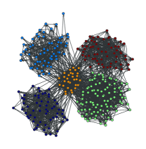
Figure 1: (Color online) Example of a network corresponding to a blockmodel with five blocks. The vertices of each block are labeled with the same color.

A stochastic blockmodel assumes that the nodes in the network can be partitioned into discrete blocks, such that every node belonging to the same block has (on average) the same characteristics. Hence, for very large systems, we need only to describe the degrees of freedom associated with the individual blocks (see Fig. 1). By considering a system composed of many blocks, we can describe a wide array of possible topological configurations.

More precisely, a (degree-corrected Karrer and Newman (2011)) stochastic blockmodel is a system of $n$ blocks, where $w_{i}$ is the fraction of nodes in the network which belong to block $i$ (we have therefore that $\sum_{i}w_{i}=1$), and $p^{i}_{k}$ is the in-degree distribution of block $i$. Thus, the average in-degree is given by ${\left<k\right>}=\sum_{k,i}kp^{i}_{k}w_{i}$. The matrix $w_{j\to i}$ describes the fraction of the inputs of block $i$ which belong to block $j$ (we have therefore that $\sum_{j}w_{j\to i}=1$). Since the out-degrees are not explicitly required to describe the dynamics (see Eq. 11 below), they will be assumed to be randomly distributed, subject only to the restrictions imposed by $w_{i}$ and $w_{j\to i}$.

We note that, although we have diminished the class of networks which will be accessible by the evolutionary algorithm, we still allow a very large array of possible configurations, which can in principle incorporate arbitrary in-degree distributions, degree correlations Newman (2003a), assortative or disassortative mixing Newman (2003b), and community structure Girvan and Newman (2002), to name only a few properties. As will become clear in the following section, this blockmodel is sufficient to characterize the most important topological property that is relevant for robustness against noise, which is the formation of densely connected central subgraphs.

IV.1 The value of $b^{*}$ for a blockmodel

Supposing that the number of vertices $Nw_{i}$ belonging to each block $i$ is arbitrarily large, we can compute the value of $b^{*}$ using an heterogeneous version of the annealed approximation Derrida and Pomeau (1986), by supposing that at each time step the inputs of each function are randomly chosen, such that the specified block structure given by $w_{i\to j}$ is always preserved Peixoto (2012). If the number of vertices in each block is large enough, we can expect this approximation to become an exact description for quenched networks as well. We can then write the average value of $b_{i}$ for each block over time as

$$b_{i}(t+1)=\sum_{k}p_{k}^{i}m_{k}\left((1-2P)\sum_{j}w_{j\to i}b_{j}(t)+P\right),$$ (11)

which is a system of $n$ coupled maps, where $m_{k}(b)$ is the probability that the output of a majority function will be $1$, if the inputs are $1$ with probability $b$, and is given by

$$m_{k}(b)=\sum_{i={\lceil k/2\rceil}}^{k}{k\choose i}b^{i}(1-b)^{k-i}.$$ (12)

A fixed point of Eq. 11 represents the solution of a polynomial system of arbitrary order, and therefore cannot be written in closed form. However, it can be obtained numerically by starting the system at $b_{i}=0$, and iterating Eq. 11 until a fixed-point $\{b^{*}_{i}\}$ is reached. The value of $b^{*}$ can then be obtained as $b^{*}=\sum_{i}w_{i}b^{*}_{i}$.

IV.2 Blockmodel entropy

We obtain the entropy of the stochastic blockmodel ensemble Bianconi (2009); Peixoto (2011) by enumerating all possible networks which are compatible with a given choice of $w_{i}$, $p_{k}^{i}$ and $w_{i\to j}$. To make the counting simpler, we ignore the difficulty of forbidding parallel edges, and consider the ensemble of configurations, since the occurrence of parallel edges should vanish for large network sizes (see Peixoto (2011) for more details). Later we compare the results obtained with Monte-Carlo simulations with parallel edges forbidden, and we find very good agreement.

We begin by enumerating all possible in-degree sequences of each block which correspond to the prescribed in-degree distributions,

$$\Omega_{d}=\prod_{i}\frac{(Nw_{i})!}{\prod_{k}{(Nw_{i}p_{k}^{i})!}}.$$ (13)

For a given block $i$ with a fixed in-degree sequence, we can count the number of different input choices as

$$\Omega^{i}_{e}=\frac{E_{i}!}{\prod_{j}E_{j\to i}!}\prod_{j}(Nw_{j})^{E_{j\to i}},$$ (14)

where $E_{i}=Nw_{i}k_{i}$ is the total number of inputs belonging to block $i$ and $E_{j\to i}=w_{j\to i}E_{i}$ is the total number of inputs from block $i$ which belong to block $j$. Since the set of inputs of each function is unordered, we still need to divide the whole number of input combinations by $\prod_{k}(k!)^{N_{k}}$, where $N_{k}=N\sum_{i,k}w_{i}p_{k}^{i}$ is the total number of vertices with in-degree $k$. Putting it all together we have

$$\Omega=\Omega_{d}\frac{\prod_{i}\Omega^{i}_{e}}{\prod_{k}(k!)^{N_{k}}}.$$ (15)

Taking the logarithm of this expression, and the limit $N\gg 1$, and using Stirling’s approximation, we obtain the full entropy (up to a trivial constant term, which is not relevant to the minimization of the free energy),

$$\mathcal{S}/N={\left<k\right>}\ln N+\sum_{i}w_{i}\mathcal{S}_{i}^{k}\\ -\sum_{i}w_{i}k_{i}\sum_{j}w_{j\to i}\ln\left(\frac{w_{j\to i}}{w_{j}}\right),$$ (16)

where $\mathcal{S}_{i}^{k}$ is an entropy term associated with the degree distribution of block $i$, and is given by

$$\mathcal{S}_{i}^{k}=-\sum_{k}p_{k}^{i}(\ln p_{k}^{i}+\ln k!).$$ (17)

IV.3 Choice of single-block in-degree distribution

We want to constrain the number of degrees of freedom in the model, such that only the average in-degree $k_{i}$ of each block is specified, not the entire distribution. In this way, graphs with many different global in-degree distributions are still possible by composing different blocks with different $k_{i}$’s, but we have a finite number of degrees of freedom per block. In order to obtain the in-degree distribution of the individual blocks, we maximize the entropy $\mathcal{S}$, with the restriction that the average in-degrees are fixed. For that, we construct the Lagrangian,

$$\Lambda=\mathcal{S}-\sum_{i}\lambda_{i}^{\prime}\left(\sum_{k}kp_{k}^{i}-k_{i}\right)-\sum_{i}\mu_{i}\left(\sum_{k}p^{i}_{k}-1\right),$$ (18)

where $\{\lambda_{i}\}$ and $\{\mu_{i}\}$ are Lagrange multipliers which keep the averages and the normalizations constant. We note that the sum over $k$ is made only over odd values of $k$, due to the imposed restrictions on the majority function. Obtaining the critical point $(\{\frac{\partial\Lambda}{\partial p^{i}_{k}}\},\{\frac{\partial\Lambda}{\partial\lambda^{\prime}_{i}}\},\{\frac{\partial\Lambda}{\partial\mu_{i}}\})=0$, and solving for $\{p^{i}_{k}\}$ one obtains,

$$p_{k}^{i}=\frac{1}{\sinh\lambda_{i}}\frac{\lambda_{i}^{k}}{k!},$$ (19)

where $k_{i}=\lambda_{i}/\tanh\lambda_{i}$. Equation 19 is a Poisson distribution, which is defined and normalized only for odd values of $k$.

This choice of $p^{i}_{k}$ is not necessarily the optimal one. In fact, it is possible to show that single-valued distributions with zero variance tend to provide the best error resilience Peixoto (2012). Nevertheless, the improvement over a Poisson distribution is very small, and the definition of Eq. 19 allows for the average $k_{i}$ to be continuously varied, which is very practical for the optimization of the free energy.

IV.4 Block splitting, decrease of entropy and the necessary number of blocks

For the blockmodel defined in this section, there are $2n+n^{2}$ variables which define the topology, where $n$ is the number of blocks. In order for arbitrary topologies to be faithfully represented by the model, one would need to make $n\to\infty$, which would render this approach impractical. However, we will show that for the purpose at hand, only a minimal number of two blocks is sufficient to fully characterize the evolutionary process, without relying on any approximations. This is due the following two facts: 1. Any possible value of $b^{*}$ can be obtained with only two blocks; 2. Any other topology with the same $b^{*}$ will invariably have a lower entropy, and thus a larger free energy. Thus the minimum of the free energy will always lie on a two-block structure.

The first fact can be shown by construction: Consider a system of two blocks, where one of them (the “core”) is smaller and much denser, and the remaining block has an average in-degree close to the global average. The inputs of the core block belong mostly to the core itself, as well as the inputs of the remaining block. By changing the density of the core block, as well as the degree of input segregation, it can be shown Peixoto (2012) that any possible value of $b^{*}$ can be achieved .

The second fact can be shown by considering a system of many blocks, and selecting any two blocks, $l$ and $m$. If all other blocks are kept intact, it can be shown that the entropy will always be larger if these two blocks are merged into an effective single block. This can be shown by partially maximizing the entropy $S$ via the Lagrangian,

$$\Lambda=\mathcal{S}-\mu\left(\sum_{i}k_{i}w_{i}-{\left<k\right>}\right)-\sum_{i}\gamma_{i}\left(\sum_{j}w_{j\to i}-1\right),$$ (20)

where $\mu$ and $\{\gamma_{i}\}$ are Lagrange multipliers which keep the average in-degree and the normalization of $w_{j\to i}$ fixed, respectively. Obtaining the critical point $(\frac{\partial\Lambda}{\partial w_{l\backslash m}},\frac{\partial\Lambda}{\partial k_{l\backslash m}},\{\frac{\partial\Lambda}{\partial w_{{l\backslash m}\to j}}\},\{\frac{\partial\Lambda}{\partial w_{j\to{l\backslash m}}}\})=0$, and solving for $w_{l\backslash m},k_{l\backslash m},\{w_{j\to l\backslash m}\},\{w_{l\backslash m\to j}\}$ one obtains,

$$k_{l}=k_{m}$$ (21)

$$\frac{w_{l\to j}}{w_{l}}=\frac{w_{m\to j}}{w_{m}}$$ (22)

$$w_{j\to l}=w_{j\to m}.$$ (23)

This corresponds to the situation where the nodes from blocks $l$ and $m$ are topologically indistinguishable, i.e. the outgoing and incoming edges are randomly distributed among the nodes of both blocks. Since any arbitrary many-block structure can be converted into a single-block by successive block merges, it follows directly that any arbitrary many-block structure can be constructed by starting from a single block, and successively splitting blocks. Thus, since the merging of blocks always increases entropy, and the splitting decreases it, the entropy of the final structure must be smaller than that of both the initial single block and the succeeding two-block network.

In order for a many-block structure to have a lower free energy than the two-block structure with the same value of $b^{*}$, it needs to have a larger entropy. But according to the above argument, networks with a larger number of blocks tend to have smaller entropy. Networks with larger entropy and number of blocks would have to be more randomized than the two-block structure, which would invariably result in a larger value of $b^{*}$. We can therefore conclude that the global minimum of the free energy always occurs for a two-block structure, and thus we need to deal with only eight variables .

V Minimization of the free energy

Although we have an analytical expression for the entropy $\mathcal{S}$, the value of $b^{*}$ cannot be obtained in closed form, and thus the same is true for $\mathcal{F}$. Therefore we must resort to a numerical computation of $b^{*}$, via the iteration of Eq. 11, and minimize $\mathcal{F}$ with a gradient descent algorithm, using finite differences. Many of these methods work only for unconstrained optimization problems, and we need to impose several constraints: The average in-degree must be fixed, and the $w_{i}$ and $w_{j\to i}$ distributions must be normalized. However we can make the problem unconstrained by using the following transformations,

$$w_{i}=\frac{e^{\widetilde{w}_{i}}}{\sum_{j}e^{\widetilde{w}_{j}}}$$ (24)

$$w_{j\to i}=\frac{e^{\widetilde{w}_{j\to i}}}{\sum_{l}e^{\widetilde{w}_{l\to i}}},$$ (25)

where $\widetilde{w}_{i}$ and $\widetilde{w}_{j\to i}$ are unconstrained real variables. Likewise we can transform $\lambda_{i}$ as

$$\widetilde{k}_{i}=\frac{e^{\widetilde{\lambda}_{i}}}{\tanh e^{\widetilde{\lambda}_{i}}}$$ (26)

$$k_{i}=c\widetilde{k}_{i}+\gamma$$ (27)

$$\lambda_{i}=k_{i}\tanh\lambda_{i},$$ (28)

where $\widetilde{\lambda}_{i}$ is also an unconstrained real variable. To obtain $\lambda_{i}$ from Eq. 28 it is simply iterated until it converges to the correct value, within some desired precision. The values of $c$ and $\gamma$ are chosen to force $k_{i}\geq 1$ and the average in-degree to a prescribed value ${\left<k\right>}$,

$$c =\frac{{\left<k\right>}}{\sum_{i}\widetilde{k}_{i}w_{i}}, \gamma =0, \text{ if }\widetilde{k}_{m}\geq 1$$ (29)

$$c =\frac{{\left<k\right>}-1}{\sum_{i}\widetilde{k}_{i}w_{i}-\widetilde{k}_{m}}, \gamma =1-c\widetilde{k}_{m},$$ otherwise,

where $\widetilde{k}_{m}=\min(\{\widetilde{k}_{i}\})$. Thus we have obtained an unconstrained minimization problem of function $\mathcal{F}$ with respect to the variables $\{\widetilde{w}_{i}\}$, $\{\widetilde{w}_{j\to i}\}$, $\{\widetilde{\lambda}_{i}\}$.

In order to find the minimum of Eq. 10, we employed the L-BFGS quasi-Newton algorithm Byrd et al. (1995), with the gradient computed by finite differences.

VI Structural phase transition

The minimization of the free energy leads to one of two possible structures (see Fig. 2): 1. For low values of $\beta$ the topology is a fully random graph; 2. For larger values of $\beta$ there is the emergence of a segregated core structure, where one of the blocks has a larger in-degree density and is more responsible for the regulation of the whole network.

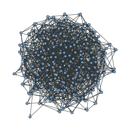
Random topology

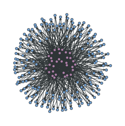
$\xrightarrow{\text{increasing }\beta}$ Segregated core

Figure 2: (Color online) Structural phase transition observed when varying the selective pressure $\beta$, as described in the text.

In order to precisely characterize the phase transition, we define the following order parameter,

$$\phi=\frac{b^{*}-b_{r}}{b_{\text{min}}-b_{r}},$$ (30)

where $b_{r}$ is the value of $b^{*}$ for a fully random network, and $b_{\text{min}}$ is the smallest possible value of $b^{*}$ for a given ${\left<k\right>}$ Peixoto (2012), given by

$$b_{\text{min}}=\sum_{k}p_{k}m_{k}(P),$$ (31)

where $p_{k}$ is given by Eq. 19 with $k_{i}={\left<k\right>}$. We have therefore that $\phi\in[0,1]$ and if $\phi=0$ the network ensemble must be fully random, and if $\phi=1$ it has the largest possible value of fitness.

As can be seen in Fig. LABEL:fig:diag-op, there is a second-order phase transition at a critical value $\beta^{*}$, which depends on the noise level $P$. The dependence of $\beta^{*}$ on $P$ divides the $\beta\times P$ phase diagram into an upper and lower branch, as can be seen in Fig. LABEL:fig:diag-phi. The branches are divided at a value of $P=P^{*}_{r}$, which is the critical value of noise of a fully random network (see Peixoto (2012) for an exact calculation of $P^{*}_{r}$). At this value of noise, a random network undergoes a dynamic phase transition, where the steady state error fraction reaches the maximum level $b^{*}=1/2$, and the dynamics become ergodic, as was described previously. For $P<P^{*}_{r}$, random networks are intrinsically robust, since $b^{*}<1/2$, and the critical value $\beta^{*}$ becomes larger with smaller $P$. In other words, the smaller is the value of noise $P$, the better is the behavior of fully random networks, such that the entropic cost of providing further improvement by creating a segregated core becomes larger, which therefore occurs only at larger values of selective pressure. The situation changes for $P>P^{*}_{r}$. Since random networks are no longer resilient, and have collapsed onto $b^{*}=1/2$ (see Fig. LABEL:fig:diag-pc), a segregated core provides a significant improvement, for a relatively low entropic cost. This cost increases with $P$, since the core needs to be either denser, smaller or more isolated to provide the same benefit under larger noise. Thus the value of $\beta^{*}$ also increases with $P$. Interestingly, in the vicinity of $P=P^{*}_{r}$, the value of $\beta^{*}$ tends to zero. For this value of noise, the dynamics of the fully random topology lies exactly at the critical point where $b^{*}=1/2$, and even the smallest (structural) perturbation can move the fixed point appreciably. Since such small structural perturbations have negligible entropic cost, the value of $\beta^{*}$ vanishes to zero. Thus, networks with ${\left<k\right>}$ such that $P^{*}_{r}=P$ are the most easily evolvable.

The value of $b^{*}$ itself can be seen in Fig. LABEL:fig:diag-pc. The upper branch $P>P^{*}_{r}$ corresponds to transitions from $b^{*}=1/2$ (ergodic dynamics) to $b^{*}<1/2$ (nonergodic dynamics), whereas the lower branch $P<P^{*}_{r}$ shows $b^{*}<1/2$ for both phases.

The topological properties of each phase can be seen in detail in Fig. LABEL:fig:diag-top, where are shown the average in-degrees $\{k_{i}\}$, block sizes $\{w_{i}\}$ and the total fraction of inputs which lead to the segregated core, $E_{c}=\sum_{j}w_{c\to j}w_{j}k_{j}/{\left<k\right>}$, where $c$ is the core block. The core block emerges at $\beta=\beta^{*}$, with an infinitesimal size, but with a value of $k_{i}$ which is usually significantly above average. For $P>P^{*}_{r}$ the segregated core usually has a significantly larger average in-degree than for $P<P^{*}_{r}$. The dominance and segregation of the core block increases continuously with $\beta$, reaching values close to $E_{c}=1$, for larger values of $\beta$, especially for values of $P>P^{*}_{r}$.

Each network on the evolved ensemble has a critical value of noise $P^{*}$ (different from the value of $P$ for which it was evolved), for which its dynamics undergoes the aforementioned ergodicity transition and which represents the maximum tolerable noise (see Peixoto (2012) for an exact calculation of $P^{*}$ for arbitrary blockmodels). Interestingly, the evolution of $b^{*}$ does not automatically result in larger values of $P^{*}$, as is shown in Fig. LABEL:fig:diag-pc: Some ensembles evolved under larger selective pressure possess a lower value of $P^{*}$ than others evolved under lower selective pressure (for the same value of $P$ under evolution). This means the evolution is reasonably specialized for the level of noise it is under, and the behavior of the networks under larger values of noise for which they were evolved is not automatically better than that of other networks with smaller fitness. However, despite these deviations, the general tendency is that, for larger values of $\beta$, $b^{*}$ and $P^{*}$ are decreased and increased, respectively.

VII Monte-Carlo simulations

We have also performed Monte Carlo simulations to observe the phase-transition obtained in the previous section. We employed the Metropolis-Hastings Metropolis et al. (1953); Hastings (1970) algorithm, starting from a random network with $N$ vertices, with a given average in-degree ${\left<k\right>}$ and a partition into $n$ blocks, represented by assigning block labels to each vertex (which is initially randomly chosen). At each iteration, one of the following moves is attempted with equal probability:

1. Block label move: A random vertex $v$ is chosen, and its block label is randomly chosen among all $n$ possible values.

2. Input move: A vertex $v$ is chosen with probability $p\propto k(k-1)$, where $k$ is the in-degree of $v$. Another vertex $u$ is randomly chosen with uniform probability. Two random inputs from $v$ are deleted and moved to $u$.

3. Source move: A random vertex $v$ is chosen. A random input from $v$ is deleted and replaced by a randomly chosen one.

A move is rejected if it generates parallel edges or self-loops. The difference $\Delta b^{*}$ of the value of $b^{*}$ after and before the move is computed. The move is then accepted with a probability $p_{a}$ given by

$$p_{a}=\begin{cases}1&\text{ if }\Delta b^{*}\leq 0,\\ e^{-\beta N\Delta b^{*}}&\text{ otherwise.}\end{cases}$$ (32)

The probability $p\propto k(k-1)$ in move (2) is chosen to correspond to two independent single-edge moves affecting the same vertices $v$ and $u$, where in each move a random edge is chosen, and its target is moved to a randomly chosen vertex. This guarantees that there is no topological bias, and that the in-degrees are always odd.

The value of $b^{*}$ is computed by obtaining the values of $\{w_{i}\}$, $\{w_{j\to i}\}$ and $\{k_{i}\}$, and iterating Eq. 11. This is much faster than actually measuring the error level on the network, and produces deterministic values .

Since we have employed the block label move (1), which tends to partition the network evenly into $n$ blocks of equal sizes, we have included an entropic cost associated with the size of a block, which did not exist in the original blockmodel above. In the original model, the partitions themselves are not relevant, and only the resulting graph topology contributes to the entropy. However, move (1) makes the algorithm very efficient and easy to implement, and it should not fundamentally change the results. But in order to compare with the theory, we need to include the following correction in the number of possible networks:

$$\Omega^{\prime}=\Omega\times\frac{N!}{\prod_{i}(Nw_{i})!}$$ (33)

which leads to the slightly modified entropy,

$$\mathcal{S}^{\prime}/N=\mathcal{S}/N-\sum_{i}w_{i}\ln w_{i}.$$ (34)

In Fig. LABEL:fig:mc-trans we can see the same phase transition observed previously, which matches very well the theoretical predictions. In Fig. LABEL:fig:mc-top the topology can be assessed more closely, and the emergence of the segregated core is clear. Due to the partition entropy introduced in Eq. 34, the core does not vanish at the transition; it merges continuously with the other block instead. However, the critical value $\beta^{*}$ is identical with the non-modified model.

The inclusion of the partition entropy also introduces the fact that different solutions are obtained for a different number of blocks, since this has a direct effect on the preferred sizes of the blocks (see Fig. LABEL:fig:mc-multiblock, left). However, this does not change the fact that for any number of blocks the preferred topology will always be an effective two-block structure. This follows from the argumentation presented previously based on the reduction of entropy resulting from block splits, and can be observed in simulations with many blocks, as shown in Fig. LABEL:fig:mc-top, which shows a comparison between the topologies obtained with two and three blocks, as well as the outcome of a typical simulation with $20$ blocks, which shows the eventual collapse of into an effective two-block structure.

VIII Gene regulatory networks

Here we make a comparison with some features observed in actual gene regulatory networks. We consider the networks for Saccharomyces cerevisiae (yeast) and Escherichia coli, extracted from the YEASTRACT Abdulrehman et al. (2010) and RegulonDB Gama-Castro et al. (2010) databases, respectively. We are interested in extracting the “functional core” of the network, i.e. those nodes which are solely responsible for global regulation, like those belonging to the segregated core which emerges in the phase transition observed in the evolutionary process above. We will characterize the core nodes in two ways: 1. Nodes which have an out-degree larger than zero; 2. Nodes which belong to a strongly connected component (SCC) of the graph (i.e. the maximal set of nodes which can directly or indirectly regulate each other). The first criterion is a necessary condition, since if the out-degree is zero, then a node is not a regulator. The second criterion is stronger, since even if a node is a regulator, it can have its dynamics completely enslaved by other nodes. The nodes in the SCC are exactly those which are not necessarily enslaved, and can mutually regulate each other. Without a least one SCC in the network, an autonomous behavior with dynamical attractors other than simple fixed-points is not possible.

The yeast network is composed of $N=6402$ nodes, with an average in-degree of ${\left<k\right>}\approx 7.51$. The E. coli network is smaller and sparser, with $N=1658$ and ${\left<k\right>}\approx 2.32$. In both networks the number of transcription factor (TF) genes is much smaller than the total number: $N_{\text{TF}}=182$ in yeast, and $N_{\text{TF}}=154$ in E. coli. These are core genes according to the first criterion, since they have an out-degree larger than zero, as can be seen in Fig. 10.

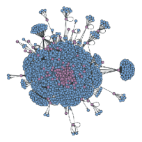
Figure 10: (Color online) Gene regulatory networks for Saccharomyces cerevisiae (left) and Escherichia coli (right), extracted from the YEASTRACT Abdulrehman et al. (2010) and RegulonDB Gama-Castro et al. (2010) databases, respectively. The nodes in purple (towards the middle) are transcription factor genes, and are the only ones with out-degree larger than zero.

In yeast, the average in-degree of the core nodes is higher than average, ${\left<k\right>}_{c}\approx 10.03$, as observed in the segregated core phase of the evolved networks obtained. For the SCC, the number of nodes decreases slightly to $N_{\text{SCC}}=146$, and the average in-degree changes negligibly ${\left<k\right>}_{CC}\approx 10.48$ (if one counts only edges between vertices of the SCC, this value is virtually identical, ${\left<k\right>}_{CC}\approx 10.42$). This is similar to what was found previously in Maslov and Sneppen (2005) for the yeast network (using an older, and less complete dataset with only $837$ genes). They have also found that the TF genes have different connection patterns, and those with the largest out-degree tend to regulate genes with lower than average in-degree. However they did not find that the TF genes form a denser subgraph, with an larger than average in-degree, which is most likely due to the incompleteness of the dataset used. Very similar numbers to those presented here were obtained more recently in Balaji et al. (2006a), using a more complete dataset (which is not identical to the one used in this work).

For E. coli the situation changes somewhat: The average in-degree of the transcription factor nodes is ${\left<k\right>}_{c}\approx 1.97$, which is in fact lower than the global average. However, if one extracts the largest SCC, the number of nodes drops dramatically to $N_{\text{SCC}}=8$. These nodes are responsible for the regulation of $411$ genes. A majority of $1093$ genes are instead enslaved to the dynamics of SCC with only two mutually regulating nodes. Although the largest SCC does have an average in-degree ${\left<k\right>}_{CC}=6$, the core topology seems significantly more sparse than for yeast and the evolved networks, at least with the data currently available Cosentino Lagomarsino et al. (2007). Arguably, such a sparse regulating core is suspect from the point of view of data set completeness, since it would mean that the range of dynamical behavior for the regulatory network is very restricted. As previously mentioned, and older and less complete data set for yeast also did not reveal a denser regulating core Maslov and Sneppen (2005). Nevertheless, one should also consider that such real networks are simultaneously under different, possibly competing selective pressures which also influence the resulting topology, robustness against noise being only one of them. These other factors, which are neglected in the model, could be one reason for such a discrepancy. We emphasize, however, that although apparently it is not denser, a regulating core certainly exists in the measured E. coli network, which is at least in partial qualitative agreement with what is observed in the model.

There are other factors that may contribute to this observed segregation which are not in principle related to noise resilience. For instance, non-regulating genes exist mostly to transcribe proteins which have some specific metabolic or structural function in the cell, and it may be difficult for these proteins to have a dual role as transcription factors, and therefore become specialized (although non-specialized proteins are not impossible, since a protein can in principle bind both to DNA and to other proteins). Nevertheless, there are good reasons to consider robustness to noise as a very plausible driving force toward this type of topology. This is corroborated, for instance, by evidence that core TF genes tend to be less noisy Fraser et al. (2004); Jothi et al. (2009), and that the vast majority of TF genes in yeast are not vital for the survival of the cell if repressed in isolation Balaji et al. (2006b). This is fully compatible with the idea of a highly redundant functional core, which provides robustness for the rest of the network.

Another feature which is commonly investigated in empirical networks is the in- and out-degree distributions. The in-degree distribution is often narrow, while the out-degree distribution is broader, and as some suggest Maslov and Sneppen (2005), compatible with a power law. The model considered in this work is parametrized as a stochastic blockmodel, where each block has in- and out-degrees that are Poisson distributed. When the segregated core emerges, the system is composed of only two blocks, thus both the in- and out-degree distributions are bimodal. The in-degree distribution is indeed narrower, since the difference between the average in-degree of the two blocks is not very large for most networks obtained. The out-degree distribution is also much broader, since the average out-degree of the non-core block tends to zero, while for the core block it tends very rapidly to infinity, when the selective pressure is increased. However, the homogeneous and seemingly scale-free properties of the empirical distributions are not reproduced by the model. This implies that these features are not a direct result of evolved robustness against noise, and may, for instance, be due simply to mutational bias caused by gene duplication, which is known to qualitatively reproduce these types of in- and out-degree distributions Ispolatov et al. (2005); Enemark and Sneppen (2007).

IX Conclusion

We have investigated the effect of selective pressure favoring robustness against noise on the structural evolution of Boolean networks with optimal majority functions, functioning as a conceptual model for gene regulation. We have mapped the evolutionary process onto a Gibbs ensemble, and obtained its outcome by minimizing the associated free energy. We showed that the structural properties of the system undergo a phase transition at a critical value of selective pressure, from a random topology to a segregated-core structure, where a smaller fraction of the nodes form an isolated core, which is denser than the rest of the network and is responsible for most of the regulation. Since the core is denser, its nodes can profit from more regulatory redundancy, which greatly diminishes the effect of noise. This robustness is propagated to the rest of the network, which relies on the core for most of the regulation. The segregated core becomes denser, smaller, and more isolated as the selective pressure increases. We have compared the theoretical predictions with Monte-Carlo simulations of actual networks, and found perfect agreement.

We have also shown that this segregated-core structure is present in the gene regulatory network of yeast and E. coli. Both networks are composed of a much smaller fraction of transcription factor genes which are responsible for all regulation. In yeast, the existing core structure is very similar qualitatively to the outcome of the evolutionary process considered, with transcription factor genes forming a denser subgraph, with an average in-degree above the average for the whole network. In E. coli the isolated transcription factor core is composed of few very small regulating cores (strongly connected components), the largest of which has only eight nodes. We conjecture that such a sparse regulating core is possibly due to data set incompleteness, since it would severely restrict the range of possible dynamical behavior for the network. A less complete data set for yeast also did not show a denser regulating core structure Maslov and Sneppen (2005), although it is clearly seen with more up-to-date datasets including more genes and interactions Balaji et al. (2006a). However, one should not rule out other selection criteria which are not incorporated in the model.

It should also be noted that regulating cores of transcription factors are a common feature of other organisms, such as Mycobacterium tuberculosis Balazsi et al. (2008). Additionally, a similar (but not identical) “bow-tie” structure was also observed in the mammalian signal transduction network Ma’ayan et al. (2005); Ma’ayan (2009), where most pathways are funneled through a central core.

It is possible to formulate other reasons for the existence of such a core structure, such as a forced specialization of genes into either transcription factors or target genes. Furthermore one should mention that the effects of noise are not always detrimental, and can in some circumstances even be beneficial Blake et al. (2006); Eldar and Elowitz (2010). Nevertheless there is compelling evidence that the core genes provide a degree of robustness to the cell. Not only are the best-connected TF nodes less noisy Fraser et al. (2004); Jothi et al. (2009), they are usually found — if removed individually — not to be vital for cell survival Balaji et al. (2006b). This corroborates the idea that one of the major functions of the regulating core is to provide robustness via redundancy.

Furthermore, aside from the direct applicability to gene regulation, we have identified a fundamental mechanism of robustness against noise, which emerges naturally when networks are randomly selected for that purpose . Although most interesting systems require more than just robustness for their functioning, it is reasonable to conclude that the emergence of regulating cores is to be expected when there is enough selective pressure favoring noise resilience.

References

- Kitano (2004) H. Kitano, Nat Rev Genet 5, 826 (2004).
- Raser and O’Shea (2005) J. M. Raser and E. K. O’Shea, Science 309, 2010 (2005).
- Maheshri and O’Shea (2007) N. Maheshri and E. K. O’Shea, Annual Review of Biophysics and Biomolecular Structure 36, 413 (2007).
- Gutkind (2000) J. S. Gutkind, Signaling networks and cell cycle control: the molecular basis of cancer and other diseases (Humana Press, 2000).
- Lestas et al. (2010) I. Lestas, G. Vinnicombe, and J. Paulsson, Nature 467, 174 (2010).
- Kauffman (1969a) S. A. Kauffman, Journal of Theoretical Biology 22, 437 (1969a).
- Kauffman (1969b) S. Kauffman, Nature 224, 177 (1969b).
- Bornholdt (2005) S. Bornholdt, Science 310, 449 (2005).
- Drossel (2008) B. Drossel, in Reviews of Nonlinear Dynamics and Complexity, Vol. 1, edited by H. G. Schuster (Wiley, 2008).
- Raj and van Oudenaarden (2008) A. Raj and A. van Oudenaarden, Cell 135, 216 (2008).
- Eldar and Elowitz (2010) A. Eldar and M. B. Elowitz, Nature 467, 167 (2010).
- Kollmann et al. (2005) M. Kollmann, L. Lovdok, K. Bartholome, J. Timmer, and V. Sourjik, Nature 438, 504 (2005).
- Li et al. (2004) F. Li, T. Long, Y. Lu, Q. Ouyang, and C. Tang, Proceedings of the National Academy of Sciences of the United States of America 101, 4781 (2004).
- Albert and Othmer (2003) R. Albert and H. G. Othmer, Journal of Theoretical Biology 223, 1 (2003).
- Chaves et al. (2005) M. Chaves, R. Albert, and E. D. Sontag, Journal of Theoretical Biology 235, 431 (2005).
- Maslov and Sneppen (2005) S. Maslov and K. Sneppen, Physical Biology 2, S94 (2005).
- Harris et al. (2002) S. E. Harris, B. K. Sawhill, A. Wuensche, and S. Kauffman, Complexity 7, 23 (2002).
- Bornholdt and Sneppen (1998) S. Bornholdt and K. Sneppen, Physical Review Letters 81, 236 (1998).
- Bornholdt and Sneppen (2000) S. Bornholdt and K. Sneppen, Proceedings of the Royal Society of London. Series B: Biological Sciences 267, 2281 (2000).
- Stern (1999) M. D. Stern, Proceedings of the National Academy of Sciences 96, 10746 (1999).
- Bassler et al. (2004) K. E. Bassler, C. Lee, and Y. Lee, Physical Review Letters 93, 038101 (2004).
- Aldana et al. (2007) M. Aldana, E. Balleza, S. Kauffman, and O. Resendiz, Journal of Theoretical Biology 245, 433 (2007).
- Szejka and Drossel (2007) Szejka and Drossel, Eur. Phys. J. B 56, 373 (2007).
- Mihaljev and Drossel (2009) T. Mihaljev and B. Drossel, The European Physical Journal B 67, 259 (2009).
- Pomerance et al. (2009) A. Pomerance, E. Ott, M. Girvan, and W. Losert, Proceedings of the National Academy of Sciences 106, 8209 (2009).
- Note (1) Another realistic source of noise are perturbations in the update sequence of nodes, since gene regulation lacks a global synchronizing clock Klemm and Bornholdt (2005). However, it can be shown that absolute robustness against this type of noise can be achieved in an independent manner, and with a very small effect to the global topological characteristics of the system Peixoto and Drossel (2009b).
- Peixoto (2010) T. P. Peixoto, Physical Review Letters 104, 048701 (2010).
- Peixoto (2012) T. P. Peixoto, Journal of Statistical Mechanics: Theory and Experiment 2012, P01006 (2012).
- Peixoto and Drossel (2009a) T. P. Peixoto and B. Drossel, Physical Review E 79, 036108 (2009a).
- Nimwegen (2006) E. Nimwegen, in Power Laws, Scale-Free Networks and Genome Biology (Springer US, Boston, MA, 2006) pp. 236–253.
- Note (2) The definition above will lead to a bias if is an even number, since if the sum happens to be exactly the output will be , arbitrarily. Alternative definitions could be used, which would remove the bias Szejka et al. (2008). However, for the analysis presented here, this is not an issue since is always odd.
- Evans and Schulman (2003) W. Evans and L. Schulman, IEEE Transactions on Information Theory 49, 3094 (2003).
- Huepe and Aldana-González (2002) C. Huepe and M. Aldana-González, Journal of Statistical Physics 108, 527 (2002).
- Ispolatov et al. (2005) I. Ispolatov, P. L. Krapivsky, and A. Yuryev, Physical Review E 71, 061911 (2005).
- Enemark and Sneppen (2007) J. Enemark and K. Sneppen, Journal of Statistical Mechanics: Theory and Experiment 11, 7 (2007).
- Callen (1985) H. B. Callen, Thermodynamics and an Introduction to Thermostatistics, 2nd ed. (Wiley, 1985).
- Holland et al. (1983) P. W. Holland, K. B. Laskey, and S. Leinhardt, Social Networks 5, 109 (1983).
- Faust and Wasserman (1992) K. Faust and S. Wasserman, Social Networks 14, 5 (1992).
- Karrer and Newman (2011) B. Karrer and M. E. J. Newman, Physical Review E 83, 016107 (2011).
- Note (3) Blockmodels are essentially equivalent to the hidden-variable model Boguñá and Pastor-Satorras (2003), when the hidden variables are discrete, and their multiplicity is smaller than the number of nodes.
- Newman (2003a) M. E. J. Newman, SIAM Review 45, 167 (2003a).
- Newman (2003b) M. E. J. Newman, Phys. Rev. E 67, 026126 (2003b).
- Girvan and Newman (2002) M. Girvan and M. E. J. Newman, Proceedings of the National Academy of Sciences 99, 7821 (2002).
- Derrida and Pomeau (1986) B. Derrida and Y. Pomeau, Europhys. Lett 1, 45–49 (1986).
- Bianconi (2009) G. Bianconi, Physical Review E 79, 036114 (2009).
- Peixoto (2011) T. P. Peixoto, arXiv:1112.6028 (2011).
- Note (4) This is not the only two-block structure which can generate arbitrary values of . In Peixoto (2012) it is shown how a bipartite “restoration” structure also achieves this, albeit less efficiently.
- Note (5) We have empirically verified this by minimizing the free energy with up to 10 blocks, and the solutions were always identical to that of the two-block case presented in the following section. The general character of the two-block topology was also verified by Monte Carlo simulations with up to blocks, as discussed later in the text (see also Fig. LABEL:fig:mc-multiblock).
- Byrd et al. (1995) R. H. Byrd, P. Lu, J. Nocedal, and C. Zhu, SIAM Journal on Scientific Computing 16, 1190 (1995).
- Metropolis et al. (1953) N. Metropolis, A. W. Rosenbluth, M. N. Rosenbluth, A. H. Teller, and E. Teller, The Journal of Chemical Physics 21, 1087 (1953).
- Hastings (1970) W. K. Hastings, Biometrika 57, 97 (1970).
- Note (6) One could argue that this may overlook the buildup of correlations in the network, since it assumes that the blocks are homogeneous and have an random in-degree distribution as given by Eq. 19. However, we are only interested in networks which have this property, which, as discussed in the text, correspond to a partial maximization of entropy when the remaining constraints are in place, so this should not be an issue. To be sure, we have compared the value of computed this way with the actual empirical value and found a very good agreement (see Fig. LABEL:fig:mc-trans).
- Abdulrehman et al. (2010) D. Abdulrehman, P. T. Monteiro, M. C. Teixeira, N. P. Mira, A. B. Lourenco, S. C. dos Santos, T. R. Cabrito, A. P. Francisco, S. C. Madeira, R. S. Aires, A. L. Oliveira, I. Sa-Correia, and A. T. Freitas, Nucleic Acids Research 39, D136 (2010).
- Gama-Castro et al. (2010) S. Gama-Castro, H. Salgado, M. Peralta-Gil, A. Santos-Zavaleta, L. Muñiz-Rascado, H. Solano-Lira, V. Jimenez-Jacinto, V. Weiss, J. S. García-Sotelo, A. López-Fuentes, L. Porrón-Sotelo, S. Alquicira-Hernández, A. Medina-Rivera, I. Martínez-Flores, K. Alquicira-Hernández, R. Martínez-Adame, C. Bonavides-Martínez, J. Miranda-Ríos, A. M. Huerta, A. Mendoza-Vargas, L. Collado-Torres, B. Taboada, L. Vega-Alvarado, M. Olvera, L. Olvera, R. Grande, E. Morett, and J. Collado-Vides, Nucleic Acids Research (2010), 10.1093/nar/gkq1110.
- Balaji et al. (2006a) S. Balaji, M. M. Babu, L. M. Iyer, N. M. Luscombe, and L. Aravind, Journal of Molecular Biology 360, 213 (2006a).
- Cosentino Lagomarsino et al. (2007) M. Cosentino Lagomarsino, P. Jona, B. Bassetti, and H. Isambert, Proceedings of the National Academy of Sciences 104, 5516 (2007).
- Fraser et al. (2004) H. B. Fraser, A. E. Hirsh, G. Giaever, J. Kumm, and M. B. Eisen, PLoS Biol 2, e137 (2004).
- Jothi et al. (2009) R. Jothi, S. Balaji, A. Wuster, J. A. Grochow, J. Gsponer, T. M. Przytycka, L. Aravind, and M. M. Babu, Molecular Systems Biology 5 (2009), 10.1038/msb.2009.52.
- Balaji et al. (2006b) S. Balaji, L. M. Iyer, L. Aravind, and M. M. Babu, Journal of Molecular Biology 360, 204 (2006b).
- Balazsi et al. (2008) G. Balazsi, A. P. Heath, L. Shi, and M. L. Gennaro, Mol Syst Biol 4 (2008), 10.1038/msb.2008.63.
- Ma’ayan et al. (2005) A. Ma’ayan, S. L. Jenkins, S. Neves, A. Hasseldine, E. Grace, B. Dubin-Thaler, N. J. Eungdamrong, G. Weng, P. T. Ram, J. J. Rice, A. Kershenbaum, G. A. Stolovitzky, R. D. Blitzer, and R. Iyengar, Science 309, 1078 (2005).
- Ma’ayan (2009) A. Ma’ayan, Journal of Biological Chemistry 284, 5451 (2009).
- Blake et al. (2006) W. J. Blake, G. Balázsi, M. A. Kohanski, F. J. Isaacs, K. F. Murphy, Y. Kuang, C. R. Cantor, D. R. Walt, and J. J. Collins, Molecular Cell 24, 853 (2006).
- Note (7) Other evolutionary, non-equilibrium pathways are also possible, see e.g. Perotti et al. (2009).
- Klemm and Bornholdt (2005) K. Klemm and S. Bornholdt, Proceedings of the National Academy of Sciences of the United States of America 102, 18414 (2005).
- Peixoto and Drossel (2009b) T. P. Peixoto and B. Drossel, Physical Review E 80, 056102 (2009b).
- Szejka et al. (2008) A. Szejka, T. Mihaljev, and B. Drossel, New Journal of Physics 10, 063009 (2008).
- Boguñá and Pastor-Satorras (2003) M. Boguñá and R. Pastor-Satorras, Physical Review E 68, 036112 (2003).
- Perotti et al. (2009) J. I. Perotti, O. V. Billoni, F. A. Tamarit, D. R. Chialvo, and S. A. Cannas, Physical Review Letters 103, 108701 (2009).