A class of interior solutions corresponding to a $(2+1)$ dimensional asymptotically anti-de Sitter spacetime

Abstract

Lower dimensional gravity has the potential of providing non-trivial and valuable insight into some of the conceptual issues arising in four dimensional relativistic gravitational analysis. The asymptotically anti-de Sitter ($2+1$) dimensional spacetime described by Ba$\tilde{n}$ados, Teitelboim and Zanelli (BTZ) which admits a black hole solution, has become a source of fascination for theoretical physicists in recent years. By suitably choosing the form of the mass function $m(r)$, we derive a new class of solutions for the interior of an isotropic star corresponding to the exterior $(2+1)$ asymptotically anti-de Sitter BTZ spacetime. The solution obtained satisfies all the regularity conditions and its simple analytical form helps us to study the physical parameters of the configuration in a simple manner.

I Introduction

It is well known that lower dimensional gravity has the potential of providing non-trivial and valuable insight into some of the conceptual issues arising in four dimensional relativistic gravitational analyses. For example, the ($2+1$) dimensional spacetime geometry described by Ba$\tilde{n}$ados, Teitelboim and ZanelliBa$\tilde{n}$ados et al (1992) (henceforth BTZ), which is asymptotically anti-de Sitter and admits a black hole solution, has become a source of fascination for theoretical physicists in recent years. The advantage here is that though the system mimics $4$-dimensional analysis, it offers less intricate set of equations to deal with. It is, therefore, crucial to find a physically reasonable interior solution corresponding to the exterior BTZ spacetime which may give us deep understanding about the nature of a gravitationally collapsing body and its consequences. Mann and RossMann and Ross (1993) analyzed the collapse of a $(2+1)$ dimensional star filled with dust ($p=0$) corresponding to the exterior BTZ spacetime and showed under what condition it might collapse to a black hole. For an incompressible fluid ($\rho=constant$), the interior solution obtained by Cruz and ZanelliCruz and Zanelli (1995) puts a bound on the maximum allowed mass for such an object. The study also claims that the collapsed stage would always be covered under its event horizon. Cruz et alCruz et al (1995) presented a new solution corresponding to an exteripr BTZ spacetime with the choice $\rho=\rho_{c}(1-r^{2}/R^{2})$, where, $\rho_{c}$ is the central density, $\rho$ is the density which is a function of the radial parameter $r$, and $R$ is the boundary of the star. Another solution has been reported by Paulo M. S$\acute{a}$Paulo M. S$\acute{a}$ (1999) where a polytropic equation of state (EOS) of the form $p=K\rho^{1+1/n}$ was assumed, where $n$ is the polytropic index and $K$ is the polytropic constant.

In this paper, we report a new class of solution corresponding to the BTZ exterior spacetime which has been obtained by assuming a particular form of the mass function $m(r)$. The solution obtained has been found to satisfy all the regularity conditions and its simple analytical form helps us to study the physical parameters of the configuration in a simple manner.

II Interior spacetime

The metric for the interior of a static spherically symmetric distribution of matter in $(2+1)$ dimensions has the standard form

$$ds^{2}=-e^{2\gamma(r)}dt^{2}+e^{2\mu(r)}dr^{2}+r^{2}d\theta^{2}.$$ (1)

We assume that the energy-momentum tensor for the matter distribution at the interior of the star is given by

$$T_{ij}=(\rho+p)u_{i}u_{j}+pg_{ij},$$ (2)

where, $\rho$ represents the energy density, $p$ is the isotropic pressure, and $u^{i}$ is the $3$-velocity of the fluid. The Einstein’s field equations with a negative cosmological constant ($\Lambda<0$), for the spacetime given in Eq. (1) together with the energy-momentum tensor given in Eq. (2), rendering $G=c=1$, yield the following independent equations

$$2\pi\rho+\Lambda = \frac{\mu^{\prime}e^{-2\mu}}{r},$$ (3)

$$2\pi p-\Lambda = \frac{\gamma^{\prime}e^{-2\mu}}{r},$$ (4)

$$2\pi p-\Lambda = e^{-2\mu}\left(\gamma^{\prime 2}+\gamma^{\prime\prime}-\gamma^{\prime}\mu^{\prime}\right),$$ (5)

where a ‘$\prime$’ denotes differentiation with respect to the radial parameter $r$. Combining Eqs. (3)-(5), we have

$$\left(\rho+p\right)\gamma^{\prime}+p^{\prime}=0,$$ (6)

which is the conservation equation in $(2+1)$ dimensions. Since the system has three independent equations involving four unknown parameters ($\rho$, $p$, $\gamma(r)$, and $\mu(r)$), we will always have one degree of freedom to solve the set of equations. In some previous works, this freedom has been utilized to model (i) a dust cloud ($p=0$) Mann and Ross (1993); (ii) a fluid of uniform density ($\rho=constant$)Cruz and Zanelli (1995); and (iii) a polytropic EOS $p=K\rho^{1+1/n}$Paulo M. S$\acute{a}$ (1999). In this paper, we choose a physically meaningful form of the mass function $m(r)$, expressible in terms of the metric function $\mu(r)$ in the form

$$2m(r)=C-e^{-2\mu(r)}-\Lambda r^{2},$$ (7)

which can be obtained by integrating Eq. (3). In Eq. (7), $C$ is an integration constant and $m(r)$ is the mass within a radial distance $r$ defined as

$$m(r)=\int_{0}^{r}2\pi\rho\tilde{r}d\tilde{r}.$$ (8)

We assume that $m(r)$ has the form

$$m(r)=\frac{1}{2}-\frac{\Lambda}{2}r^{2}-\frac{e^{-Ar^{2}}}{2},$$ (9)

which is regular at the centre, i.e., $m(r)=0$ at $r=0$, $A$ being a constant. This implies

$$2\mu(r)=Ar^{2},$$ (10)

where, without any loss of generality, we have set $C=1$. Note that, for $g_{rr}>0$, we must have

$$m(r)<\frac{1}{2}-\frac{\Lambda r^{2}}{2}.$$ (11)

From Eq. (3), the energy density is then obtained as

$$\rho=\frac{1}{2\pi}\left[Ae^{-Ar^{2}}-\Lambda\right].$$ (12)

Combining Eqs. (4), (5) and (10), we get,

$$\gamma^{\prime 2}+\gamma^{\prime\prime}-Ar\gamma^{\prime}=\frac{\gamma^{\prime}}{r},$$ (13)

which on integration yields,

$$\gamma^{\prime}=\frac{Are^{\frac{A}{2}r^{2}}}{BA+e^{\frac{A}{2}r^{2}}},$$ (14)

where $B$ is an integration constant. Further integrating Eq. (14) we get

$$\gamma=\ln[D(BA+e^{\frac{A}{2}r^{2}})],$$ (15)

where $D$ is another integration constant. The spacetime metric thus obtained is free from any central singularity problem. The isotropic pressure is then obtained as

$$p=\frac{\frac{A}{2\pi}e^{-\frac{A}{2}r^{2}}}{BA+e^{\frac{A}{2}r^{2}}}+\frac{\Lambda}{2\pi}$$ (16)

Before we analyze physical features of the model, let us write $\Lambda=-K^{2}$ to ensure that the cosmological constant always remains negative. The central density and pressure are then obtained as

$$\rho_{c}=\rho(r=0) = \frac{1}{2\pi}(A+K^{2}),$$ (17)

$$p(r=0) = \frac{1}{2\pi}\left(\frac{A}{BA+1}-K^{2}\right),~{}~{}~{}~{}~{}~{}~{}~{}~{}$$ (18)

Thus, the central density and pressure remain positive if $\frac{A}{(BA+1)}>K^{2}$. For a physically meaningful solution, the radial and tangential pressures should be decreasing functions of $r$. In our model, we have

$$\frac{d\rho}{dr}=-\frac{1}{\pi}rA^{2}e^{-Ar^{2}},$$ (19)

$$\frac{dp}{dr}=-\frac{1}{2\pi}\frac{A^{2}r}{\left(BA+e^{\frac{A}{2}r^{2}}\right)}\left[e^{-\frac{A}{2}r^{2}}+\frac{1}{\left(BA+e^{\frac{A}{2}r^{2}}\right)}\right].$$

(20)

Obviously, at $r=0$, $\frac{d\rho}{dr}=\frac{dp}{dr}=0$, and the density and pressure decrease radially outward as can be seen in Fig. (1) and (2), respectively.

The radius of the star $R$ can be obtained by letting $p(r=R)=0$ in Eq. (16), which gives

$$R=\sqrt{\frac{2}{A}\ln\left[\frac{1}{2}\left(-BA+\sqrt{B^{2}A^{2}+\frac{4A}{K^{2}}}\right)\right]}.$$ (21)

The total mass confined within the radius $R$ is obtained as

$$M_{Total}=\frac{1}{2}+\frac{K^{2}R^{2}}{2}-\frac{e^{-AR^{2}}}{2}.$$ (22)

III Exterior spacetime and matching conditions

We match the interior solution to the exterior BTZ metricBa$\tilde{n}$ados et al (1992) given by

$$ds_{+}^{2}=-\left(-M_{0}-\Lambda r^{2}\right)dt^{2}+\left(-M_{0}-\Lambda r^{2}\right)^{-1}dr^{2}+r^{2}d\theta^{2},$$ (23)

where, the parameter $M_{0}$ is the conserved charge associated with asymptotic invariance under time displacements. Continuity of $g_{tt}$, $g_{rr}$ and $\frac{\partial g_{tt}}{\partial r}$ across the circular disc joining the two matrices at $r=R$, implies

$$\left(-M_{0}-\Lambda R^{2}\right)=D^{2}\left(AB+e^{\frac{A}{2}R^{2}}\right)^{2},$$ (24)

$$\left(-M_{0}-\Lambda R^{2}\right)=e^{-AR^{2}},$$ (25)

$$-2\Lambda R=2D^{2}\left(AB+e^{\frac{A}{2}R^{2}}\right)e^{\frac{A}{2}R^{2}}AR.$$ (26)

Solving the above set of equations simultaneously, we get

$$A = -\frac{1}{R^{2}}\ln\left(K^{2}R^{2}-M_{0}\right),$$ (27)

$$D = \frac{-K^{2}R^{2}}{\ln\left(K^{2}R^{2}-M_{0}\right)},$$ (28)

$$B = \frac{\left[(K^{2}R^{2}-M_{0})+\frac{K^{2}R^{2}}{\ln\left(K^{2}R^{2}-M_{0}\right)}\right]}{K^{2}\sqrt{\left(K^{2}R^{2}-M_{0}\right)}}.$$ (29)

We demand that the following energy conditions should be satisfied by the distribution: (i) $\rho,~{}p\geq 0$, (ii) $\rho+p\geq 0$ and (iii) $\rho+2p\geq 0$. Employing these energy conditions at the centre ($r=0$), we note that the first condition will be satisfied if $\frac{A}{(BA+1)}>K^{2}$, the second condition will be satisfied if $A\geq 0$, and the third condition demands that $A+\frac{2A}{(BA+1)}>K^{2}$.

To understand behaviour of the physical parameters in our model, we assume $A=0.5$, $B=0.05$, $\Lambda=-0.0625$ satisfying the above conditions. Solving Eqs. (27) and (29), we then get $R=2.035$, $M_{0}=0.1327$. With these values, variations of the physical parameters like energy density, pressure and mass function have been shown in Fig. (1), (2) and (3), respectively.

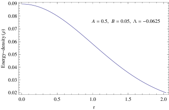
Figure 1: Density variation at the stellar interior.

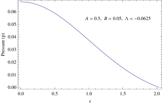
Figure 2: Pressure variation at the stellar interior.

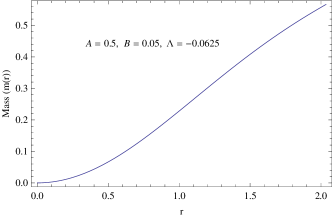
Figure 3: Variation of mass function at stellar interior.

IV Some features

IV.1 Maximum mass-radius relation

The upper bound on the mass in our model can be obtained from the observation that

$$2m(r)\equiv 1+K^{2}r^{2}-e^{-Ar^{2}}\leq 1+K^{2}r^{2}-e^{-AR^{2}},$$ (30)

which implies

$$\left(\frac{m}{r}\right)_{max}\equiv\frac{M}{R}\leq\frac{1+K^{2}R^{2}-e^{-AR^{2}}}{2R}.$$ (31)

To see the maximum allowable mass-radius ratio in our model, we plot $\frac{m(r)}{r}$ against $r$ (see Fig. 4) which shows that the ratio $\frac{m(r)}{r}$ is an increasing function of the radial parameter. We note that a constraint on the maximum allowed mass-radius ratio in our case falls within the limit to the (3+1) dimensional case of isotropic fluid sphere i.e., $\left(\frac{m}{r}\right)_{max}=0.278<\frac{4}{9}$.

IV.2 Compactness

The compactness of the star is given by

$$u=\frac{m(r)}{r}=\frac{1}{2r}\left(1+K^{2}r^{2}-e^{-Ar^{2}}\right).$$ (32)

The surface redshift ($Z_{s}$) corresponding to the above compactness ($u$) is obtained as

$$Z_{s}=(1-2u)^{-\frac{1}{2}}-1,$$ (33)

where

$$Z_{s}=\left[1-\frac{1}{r}\left(1+K^{2}r^{2}-e^{-Ar^{2}}\right)\right]^{-\frac{1}{2}}-1.$$ (34)

Thus, the maximum surface redshift of our (2+1) dimensional star of radius $R=2.035$ turns out to be $Z_{s}=0.51$.

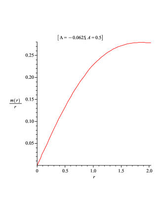
Figure 4: The variation of $\frac{m(r)}{r}$ is shown against r.

IV.3 Sound speed

For a physically acceptable model, one expects that the velocity of sound $v_{s}=(dp/d\rho)^{\frac{1}{2}}$ should be within the range $0\leq v_{s}^{2}<1$. In our model

$$v_{s}^{2}=\frac{1}{2}\frac{e^{Ar^{2}}}{\left(BA+e^{\frac{A}{2}r^{2}}\right)}\left[e^{-\frac{A}{2}r^{2}}+\frac{1}{\left(BA+e^{\frac{A}{2}r^{2}}\right)}\right].$$ (35)

We plot the radial sound speed in Fig. (5) and observe that this parameter satisfies the inequalities $0<v_{s}^{2}<1$.

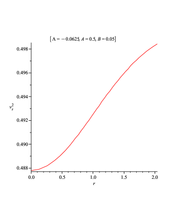
Figure 5: The variation of radial sound speed $v_{s}^{2}$ is shown against $r$.

IV.4 Equilibrium configuration

In Section III, we have matched the interior solution to the exterior BTZ metricBa$\tilde{n}$ados et al (1992) across the junction surface $S$ where $r=R$. In our case, the junction surface is a one dimensional ring of matter. Though the metric coefficients are continuous across the surface, their derivatives may not be continuous at the surface. In other words, the affine connections may be discontinuous at the boundary surface. This can be taken care of if we consider the second fundamental forms of the boundary shell. Let, $\eta$ denotes the Riemann normal coordinate at the junction which has positive signature in the manifold described by exterior BTZ spacetime and negative signature in the manifold described by the interior spacetime. Mathematically, we have $x^{\mu}=(\tau,\phi,\eta)$ and the normal vector components $\xi^{\mu}=(0,0,1)$ with the metric

$$g_{\eta\eta}=1,~{}~{}g_{\eta i}~{}=~{}0~{}~{}and~{}~{}g_{ij}=~{}diag~{}(~{}-1,~{}r^{2}~{})~{}.$$

The second fundamental forms associated with the two sides of the shell Israel (1966); Rahaman (2006, 2009); Usmani (2010); Rahaman (2010, 2011); perry (1992) are then given by

$$K^{i\pm}_{j}=\frac{1}{2}\left(g^{ik}\frac{\partial g_{kj}}{\partial\eta}\right)_{\eta=\pm 0}=\frac{1}{2}\left[\frac{\partial r}{\partial\eta}~{}g^{ik}\frac{\partial g_{kj}}{\partial r}\right]_{r=R}.$$ (36)

The discontinuity in the second fundamental forms is denoted by

$$\kappa_{ij}=K^{+}_{ij}-K^{-}_{ij}.$$ (37)

Now, from Lanczos equation in (2+1) dimensional spacetime, one can obtain the surface stress energy tensor $S_{j}^{i}=diag(-\sigma,-v)$ where, $\sigma$ and $v$ are line energy density and line tension, respectively perry (1992)

$$\sigma = -\frac{1}{8\pi}\kappa_{\phi}^{\phi},$$ (38)

$$v = -\frac{1}{8\pi}\kappa_{\tau}^{\tau}.$$ (39)

Employing Eq. (36), we get

$$\sigma = -\frac{1}{8\pi R}\left[\sqrt{K^{2}R^{2}-M_{0}}+e^{-\frac{1}{2}AR^{2}}\right],$$ (40)

$$v = -\frac{1}{8\pi}\left[\frac{K^{2}R}{\sqrt{K^{2}R^{2}-M_{0}}}+\frac{AR}{BA+e^{\frac{1}{2}AR^{2}}}\right]$$ (41)

where, we have set $r=R$. We note that the line tension is negative which implies that there must be a line pressure as opposed to the line tension. As we match the second fundamental forms, a crucial question arises in the form of the star’s stability against collapse. Therefore, we must have a thin ring of matter component with above stresses so that the outer boundary exerts outward force to balance the inward pull of BTZ exterior. The energy density is negative in this junction ring which is similar to the $(3+1)$ dimensional caseVisser1989 .

V Discussion

We have obtained a new class of solution corresponding to the BTZ exterior spacetime by assuming a particular form of the mass function $m(r)$. The solution obtained is regular at the centre and it satisfies all the physical requirements except at the boundary where we propose a thin ring of matter content with negative energy density so as to prevent collapsing. The discontinuity of the affine connections at the boundary surface provide the above matter confined to the ring. Such a stress-energy tensor is not ruled out from the consideration Casimir effect for massless fields. The solution obtained here has a simple analytical form which can be used to study a full collapsing model of a $(2+1)$ dimensional star which is beyond the scope of this analysis. This will be taken up else where.

References

- Baados et al (1992) M. Baados, C. Teitelboim and J. Zanelli, Phys. Rev. Lett. 69, 1849 (1992).
- Mann and Ross (1993) R. B. Mann and S. F. Ross, Phys. Rev. D 47, 3319 (1993).
- Cruz and Zanelli (1995) N. Cruz and J. Zanelli, Class. Quant. Grav. 12, 975 (1995).
- Cruz et al (1995) N. Cruz, M. Olivares and J. R. Villanueva, Gen. Relativ. Grav. 37, 667 (2004).
- Paulo M. S (1999) Paulo M. S, Phys. Lett. B467, 40 (1999).
- Israel (1966) W. Israel, Nuo. Cim. B 44, 1 (1966); erratum - ibid. 48B, 463 (1967).
- Usmani (2010) A. A. Usmani, Z. Hasan, F. Rahaman, Sk. A. Rakib, S. Ray, P. K. F. Kuhfittig, Gen. Relativ. Grav. 42, 2901 (2010).
- Rahaman (2010) F. Rahaman, K. A. Rahman, Sk. A Rakib, P. K. F. Kuhfittig, Int. J. Theor. Phys. 49, 2364 (2010).
- Rahaman (2006) F. Rahaman et al., Gen. Relativ. Grav. 38, 1687 (2006).
- Rahaman (2009) F. Rahaman et al., Acta Phys.Polon. B40, 1575 (2009).
- Rahaman (2011) F. Rahaman, P. K. F. Kuhfittig, M. Kalam, A. A. Usmani and S. Ray, Class. Quant. Grav. 28, 155021 (2011).
- perry (1992) G. P. Perry and R. B. Mann, Gen. Relativ. Grav. 24, 305 (1992).
- (13) M. Visser, Nucl. Phys. B 328, 203 (1989).