A fractional Feynman-Kac equation for weak ergodicity breaking

Abstract

Continuous-time random walk (CTRW) is a model of anomalous sub-diffusion in which particles are immobilized for random times between successive jumps. A power-law distribution of the waiting times, $\psi(\tau)\sim\tau^{-(1+\alpha)}$, leads to sub-diffusion ($\left\langle x^{2}\right\rangle\sim t^{\alpha}$) for $0<\alpha<1$. In closed systems, the long stagnation periods cause time-averages to divert from the corresponding ensemble averages, which is a manifestation of weak ergodicity breaking. The time-average of a general observable $\overline{U}=\frac{1}{t}\int_{0}^{t}U[x(\tau)]d\tau$ is a functional of the path and is described by the well known Feynman-Kac equation if the motion is Brownian. Here, we derive forward and backward fractional Feynman-Kac equations for functionals of CTRW in a binding potential. We use our equations to study two specific time-averages: the fraction of time spent by a particle in half box, and the time-average of the particle’s position in a harmonic field. In both cases, we obtain the probability density function of the time-averages for $t\rightarrow\infty$ and the first two moments. Our results show that indeed, both the occupation fraction and the time-averaged position are random variables even for long-times, except for $\alpha=1$ when they are identical to their ensemble averages. Using the fractional Feynman-Kac equation, we also study the dynamics leading to weak ergodicity breaking, namely the convergence of the fluctuations to their asymptotic values.

I Introduction

The time-average of an observable $U(x)$ of a diffusing particle is defined as

$$\overline{U}=\frac{1}{t}\int_{0}^{t}U[x(\tau)]d\tau,$$ (1)

where $x(t)$ is the particle’s trajectory. For Brownian motion in a binding potential $V(x)$ and in contact with a heat bath, ergodicity leads to

$$\lim_{t\rightarrow\infty}\overline{U}=\left\langle U\right\rangle_{\textrm{th}}=\int_{-\infty}^{\infty}U(x)G_{\textrm{eq}}(x)dx,$$ (2)

where $G_{\textrm{eq}}(x)=e^{-V(x)/(k_{B}T)}/Z$ is Boltzmann distribution and $\left\langle U\right\rangle_{\textrm{th}}$ is the thermal average. The equality of time- and ensemble averages in ergodic systems is one of the basic presuppositions of statistical mechanics.

In the last decades it was found that in many systems, the diffusion of particles is anomalously slow, as characterized by the relation $\left\langle x^{2}\right\rangle\sim t^{\alpha}$ with $0<\alpha<1$ Havlin ; Bouchaud ; KlafterReview2000 ; AnomalousTransportBook . Anomalous sub-diffusion is commonly modeled as a continuous-time random walk (CTRW): nearest-neighbor hopping on a lattice, with waiting times between jumps distributed as a power-law with infinite mean MontrollWeiss ; ScherMontroll .

For closed systems, the long immobilization periods of CTRW result in deviation of time-averages from ensemble averages even for long times BarkaiPRL05 ; BarkaiJSP06 ; BarkaiPRL07 ; BarkaiJSP08 . Although there are no inaccessible regions in the phase space (i.e., there is no strong ergodicity breaking), the divergence of the mean waiting time results in some waiting times of the order of magnitude of the entire experiment. Therefore, a particle does not sample the phase space uniformly in any single experiment, leading to weak ergodicity breaking BouchaudWEB .

Two examples of particularly interesting time-averages, which we study in this paper, are given below. For a particle in a bounded region, the occupation fraction is defined as $\lambda=\frac{1}{t}\int_{0}^{t}\Theta[x(\tau)]d\tau$, namely, it is the fraction of time spent by the particle in the positive side of the region GrebenkovPRE ; OccTimeMajumdarPRL . Generally, the occupation fraction can be defined for any given subspace. Consider, for example, a particle in a sample illuminated by a laser, where the particle emits photons only when it is under the laser’s focus. The occupation fraction is proportional to the total emitted light OccupationExeperimental ; AgmonResidenceMoments . Next, the time-averaged position of a particle is defined as $\overline{x}=\frac{1}{t}\int_{0}^{t}x(\tau)d\tau$. Recent advances in single particle tracking technologies enable the experimental determination of the time-average of the position of beads in polymer networks AnomalousBeads1 ; AnomalousBeads2 and of biological macro-molecules and small organelles in living cells AnomalousDNA ; AnomalousTelomere ; AnomalousmRNA ; AnomalousLipid1 . Since in many physical and biological systems the diffusion is anomalous, the study of occupation fractions or time-averaged positions in sub-diffusive processes such as CTRW is of current interest.

Time-averages are closely related to functionals, which are defined as $A=\int_{0}^{t}U[x(\tau)]d\tau$ and have many applications in physics, mathematics and other fields MajumdarReview . Denote by $G(x,A,t)$ the joint PDF of finding, at time $t$, the particle at $x$ and the functional at $A$. The Feynman-Kac equation states that for a free Brownian particle Kac1949 :

$$\frac{\partial}{\partial t}G(x,p,t)=K_{1}\frac{\partial^{2}}{\partial x^{2}}G(x,p,t)-pU(x)G(x,p,t),$$ (3)

where $G(x,p,t)$ is the Laplace transform $A\rightarrow p$ of $G(x,A,t)$ and $K_{1}$ is the diffusion coefficient. Recently, we developed a fractional Feynman-Kac equation for anomalous diffusion of free particles BarkaiPRL09 ; BarkaiJSP10 . As time-averages are in fact scaled functionals: $\overline{U}=A/t$, a generalized Feynman-Kac equation for anomalous functionals in a binding field would be invaluable for the study of weak ergodicity breaking. Currently, no such equation exists and weak ergodicity breaking was investigated only in the $t\rightarrow\infty$ limit or using functional- and potential-specific methods BarkaiPRL05 ; BarkaiJSP06 ; BarkaiPRL07 ; BarkaiJSP08 .

In this paper, we obtain an equation for functionals of anomalous diffusion in a force field $F(x)$. The equation takes the following form (reported without derivation in BarkaiPRL09 ):

$$\frac{\partial}{\partial t}G(x,p,t)=$$ (4)

$$K_{\alpha}\left[\frac{\partial^{2}}{\partial x^{2}}-\frac{\partial}{\partial x}\frac{F(x)}{k_{B}T}\right]{\cal D}_{t}^{1-\alpha}G(x,p,t)-pU(x)G(x,p,t).$$

The symbol ${\cal D}_{t}^{1-\alpha}$ is a fractional substantial derivative, equal in Laplace $t\rightarrow s$ space to $[s+pU(x)]^{1-\alpha}$ FriedrichPRL06 ; FriedrichPRE06 , and $K_{\alpha}$ is a generalized diffusion coefficient. Solving Eq. (4) for $G(x,p,t)$, inverting $p\rightarrow A$ and integrating over all $x$ yields $G(A,t)$, the PDF of $A$ at time $t$. Changing variables $A\rightarrow A/t=\overline{U}$, one finally comes by $G(\overline{U},t)$, the (time-dependent) PDF of $\overline{U}$. Weak ergodicity breaking can then be determined by looking at the long-times properties of $G(\overline{U},t)$: if $\overline{U}$ is not identically equal to $\left\langle U\right\rangle_{\textrm{th}}$ for $t\rightarrow\infty$, ergodicity is broken. Moreover, if $G(\overline{U},t)$ or the moments of $\overline{U}$ can be found also for $t<\infty$, the kinetics of weak ergodicity breaking can be uncovered.

In the rest of the paper, we derive Eq. (4) as well as a backward equation and an equation for time-dependent forces. We then apply our equation to the two examples given above: the occupation fraction in a box and the time-averaged position in a harmonic potential. In both cases, we calculate the long-times limit of $G(\overline{U},t)$ and the fluctuations $\left\langle(\Delta\overline{U})^{2}\right\rangle=\left\langle\overline{U}^{2}\right\rangle-\left\langle\overline{U}\right\rangle^{2}$. We demonstrate that for sub-diffusion both systems exhibit weak ergodicity breaking, and that the fluctuations decay as $t^{-\alpha}$ to their asymptotic limit. Part of the results for the fluctuations of the time-averaged position were briefly reported in BarkaiPRL09 .

II Derivation of the fractional equations

II.1 The forward equation

II.1.1 Continuous-time random walk

In the continuous-time random walk model, a particle is placed on an one-dimensional lattice with spacing $a$ and is allowed to jump to its nearest neighbors only. The probabilities of jumping left $L(x)$ and right $R(x)$ depend on $F(x)$, the force at $x$ (see next subsection for derivation of these probabilities). If $F(x)=0$, then $R(x)=L(x)=1/2$. Waiting times between jump events are independent identically distributed random variables with PDF $\psi(\tau)$, and are independent of the external force. The initial position of the particle, $x_{0}$, is distributed according to $G_{0}(x)$. The particle waits in $x_{0}$ for time $\tau$ drawn from $\psi(\tau)$, and then jumps to either $x_{0}+a$ (with probability $R(x)$) or $x_{0}-a$ (with probability $L(x)$), after which the process is renewed. We assume that the waiting time PDF scales as

$$\psi(\tau)\sim\frac{B_{\alpha}}{|\Gamma(-\alpha)|}\tau^{-(1+\alpha)},$$ (5)

where $0<\alpha<1$. With this PDF, the mean waiting time is infinite and the process is sub-diffusive: for $F(x)=0$, $x_{0}=0$, and for an infinite open system, $\left\langle x^{2}\right\rangle\sim t^{\alpha}$ BarkaiPRE00 . We also consider the case when the mean waiting time is finite, e.g., an exponential distribution $\psi(\tau)=e^{-\tau/\left\langle\tau\right\rangle}/\left\langle\tau\right\rangle$. This leads to normal diffusion $\left\langle x^{2}\right\rangle\sim t$ and we therefore refer to this case as $\alpha=1$. For discussion on the effect of an exponential cutoff on Eq. (5), see WaitingTimeCutoff . Below, we derive the differential equation that describes the distribution of functionals in the continuum limit of this model.

II.1.2 Derivation of the equation

Define $A=\int_{0}^{t}U[x(\tau)]d\tau$ and define $G(x,A,t)$ as the joint PDF of $x$ and $A$ at time $t$. For the particle to be at $(x,A)$ at time $t$, it must have been at $[x,A-\tau U(x)]$ at time $t-\tau$ when the last jump was made. Let $\chi(x,A,t)dt$ be the probability of the particle to jump into $(x,A)$ in the time interval $[t,t+dt]$. We have,

$$G(x,A,t)=\int_{0}^{t}W(\tau)\chi[x,A-\tau U(x),t-\tau]d\tau,$$ (6)

where $W(\tau)=1-\int_{0}^{\tau}\psi(\tau^{\prime})d\tau^{\prime}$ is the probability for not moving in a time interval of length $\tau$.

To calculate $\chi$, note that to arrive to $(x,A)$ at time $t$, the particle must have arrived to either $[x-a,A-\tau U(x-a)]$ or $[x+a,A-\tau U(x+a)]$ at time $t-\tau$ when the previous jump was made. Therefore,

$$\chi(x,A,t)=G_{0}(x)\delta(A)\delta(t)$$ (7)

$$+\int_{0}^{t}\psi(\tau)L(x+a)\chi[x+a,A-\tau U(x+a),t-\tau]d\tau$$

$$+\int_{0}^{t}\psi(\tau)R(x-a)\chi[x-a,A-\tau U(x-a),t-\tau]d\tau.$$

The term $G_{0}(x)\delta(A)\delta(t)$ corresponds to the initial condition, namely that at $t=0$, $A=0$ and the particle’s position is distributed as $G_{0}(x)$.

Assume that $U(x)\geq 0$ for all $x$ and thus $A\geq 0$ (an assumption we will relax in Section II.1.3). Let $\chi(x,p,t)=\int_{0}^{\infty}e^{-pA}\chi(x,A,t)dA$ be the Laplace transform $A\rightarrow p$ of $\chi(x,A,t)$ (we use along this work the convention that the variables in parenthesis define the space we are working in). Laplace transforming Eq. (7) from $A$ to $p$, we find

$$\chi(x,p,t)=G_{0}(x)\delta(t)$$ (8)

$$+L(x+a)\int_{0}^{t}\psi(\tau)e^{-p\tau U(x+a)}\chi(x+a,p,t-\tau)d\tau$$

$$+R(x-a)\int_{0}^{t}\psi(\tau)e^{-p\tau U(x-a)}\chi(x-a,p,t-\tau)d\tau.$$

Laplace transforming Eq. (8) from $t$ to $s$ using the convolution theorem,

$$\chi(x,p,s)=G_{0}(x)$$ (9)

$$+L(x+a)\hat{\psi}[s+pU(x+a)]\chi(x+a,p,s)$$

$$+R(x-a)\hat{\psi}[s+pU(x-a)]\chi(x-a,p,s),$$

where $\hat{\psi}(s)$ is the Laplace transform of the waiting time PDF. Let $\chi(k,p,s)=\int_{-\infty}^{\infty}e^{ikx}\chi(x,p,s)dx$ be the Fourier transform $x\rightarrow k$ of $\chi$. Fourier transforming Eq. (9) and changing variables $x\pm a\rightarrow x$,

$$\chi(k,p,s)=\hat{G}_{0}(k)$$ (10)

$$+e^{-ika}\int_{-\infty}^{\infty}e^{ikx}L(x)\hat{\psi}[s+pU(x)]\chi(x,p,s)dx$$

$$+e^{ika}\int_{-\infty}^{\infty}e^{ikx}R(x)\hat{\psi}[s+pU(x)]\chi(x,p,s)dx,$$

where $\hat{G}_{0}(k)$ is the Fourier transform of the initial condition.

We now express $L(x)$ and $R(x)$ in terms of the potential $V(x)$. Assuming the system is coupled to a heat bath at temperature $T$ and assuming detailed balance, we have BarkaiPRE00 ; BarkaiJSP08

$$L(x)\exp\left[-\frac{V(x)}{k_{B}T}\right]=R(x-a)\exp\left[-\frac{V(x-a)}{k_{B}T}\right].$$ (11)

If the lattice spacing $a$ is small we can expand

$$\exp\left[-\frac{V(x-a)}{k_{B}T}\right]\approx\exp\left[-\frac{V(x)}{k_{B}T}\right]\left[1-\frac{aF(x)}{k_{B}T}+{\cal O}(a^{2})\right],$$ (12)

where we used $F(x)=-V^{\prime}(x)$. Expanding $R(x)$ and $L(x)$ for $\frac{aF(x)}{(k_{B}T)}\ll 1$, using the fact that $R(x)=L(x)=1/2$ for $F(x)=0$,

$$R(x)\approx\frac{1}{2}\left[1+c\frac{aF(x)}{k_{B}T}\right]=1-L(x),$$ (13)

where $c$ is a constant to be determined. Combining Eqs. (11), (12), and (13), we have, up to first order in $a$

$$1-c\frac{aF(x)}{k_{B}T}\approx\left[1-\frac{aF(x)}{k_{B}T}\right]\left[1+c\frac{aF(x)}{k_{B}T}\right]$$

This gives, again up to first order in $a$, $c=1/2$. We can thus write,

$$R(x)\approx\frac{1}{2}\left[1+\frac{aF(x)}{2k_{B}T}\right]\;;\;L(x)\approx\frac{1}{2}\left[1-\frac{aF(x)}{2k_{B}T}\right].$$ (14)

Substituting Eq. (14) in Eq. (10), we obtain,

$$\chi(k,p,s)\approx\hat{G}_{0}(k)$$

$$+\frac{1}{2}e^{-ika}\int_{-\infty}^{\infty}e^{ikx}\hat{\psi}[s+pU(x)]\chi(x,p,s)dx$$

$$-\frac{1}{2}e^{-ika}\int_{-\infty}^{\infty}e^{ikx}\frac{aF(x)}{2k_{B}T}\hat{\psi}[s+pU(x)]\chi(x,p,s)dx$$

$$+\frac{1}{2}e^{ika}\int_{-\infty}^{\infty}e^{ikx}\hat{\psi}[s+pU(x)]\chi(x,p,s)dx$$

$$+\frac{1}{2}e^{ika}\int_{-\infty}^{\infty}e^{ikx}\frac{aF(x)}{2k_{B}T}\hat{\psi}[s+pU(x)]\chi(x,p,s)dx.$$

Applying the Fourier transform identity ${\cal F}\{xf(x)\}=-i\frac{\partial}{\partial k}f(k)$, the last equation simplifies to

$$\chi(k,p,s)\approx\hat{G}_{0}(k)+ \left[\cos(ka)+i\sin(ka)\frac{aF\left(-i\frac{\partial}{\partial k}\right)}{2k_{B}T}\right]\times$$

$$\hat{\psi}\left[s+pU\left(-i\frac{\partial}{\partial k}\right)\right]\chi(k,p,s).$$ (15)

The symbols $F\left(-i\frac{\partial}{\partial k}\right)$ and $U\left(-i\frac{\partial}{\partial k}\right)$ represent the original functions $F(x)$ and $U(x)$, but with $-i\frac{\partial}{\partial k}$ as their arguments. Note that the order of the terms is important: for example, $\cos(ka)$ does not commute with $\hat{\psi}\left[s+pU\left(-i\frac{\partial}{\partial k}\right)\right]$. The formal solution of Eq. (II.1.2) is

$$\chi(k,p,s)\approx \left\{1-\left[\cos(ka)+i\sin(ka)\frac{aF\left(-i\frac{\partial}{\partial k}\right)}{2k_{B}T}\right]\right.\times$$

$$\left.\hat{\psi}\left[s+pU\left(-i\frac{\partial}{\partial k}\right)\right]\right\}^{-1}\hat{G}_{0}(k).$$ (16)

We next use our expression for $\chi$ to calculate $G(x,A,t)$. Transforming Eq. (6) $(x,A,t)\rightarrow(k,p,s)$,

$$G(k,p,s)=\frac{1-\hat{\psi}\left[s+pU\left(-i\frac{\partial}{\partial k}\right)\right]}{s+pU\left(-i\frac{\partial}{\partial k}\right)}\chi(k,p,s),$$ (17)

where we used the fact that $\hat{W}(s)=[1-\hat{\psi}(s)]/s$. Substituting Eq. (II.1.2) into (17), we have

$$G(k,p,s)\approx\frac{1-\hat{\psi}\left[s+pU\left(-i\frac{\partial}{\partial k}\right)\right]}{s+pU\left(-i\frac{\partial}{\partial k}\right)}\times$$ (18)

$$\left\{1-\left[\cos(ka)+i\sin(ka)\frac{aF\left(-i\frac{\partial}{\partial k}\right)}{2k_{B}T}\right]\right.\times$$

$$\left.\hat{\psi}\left[s+pU\left(-i\frac{\partial}{\partial k}\right)\right]\right\}^{-1}\hat{G}_{0}(k).$$

To derive a differential equation for $G(x,p,t)$, we use the small $s$ expansion of $\hat{\psi}(s)$. For $0<\alpha<1$, where the waiting time PDF is $\psi(\tau)\sim B_{\alpha}\tau^{-(1+\alpha)}/|\Gamma(-\alpha)|$ (Eq. (5)), the Laplace transform for small $s$ is KlafterReview2000

$$\hat{\psi}(s)\approx 1-B_{\alpha}s^{\alpha}.$$ (19)

The case $\alpha=1$ is also described by Eq. (19), if we identify $B_{1}$ with the mean waiting time $\left\langle\tau\right\rangle$. Substituting Eq. (19) in Eq. (18), and using $\cos(ka)\approx 1-k^{2}a^{2}/2$ and $\sin(ka)\approx ka$, we obtain

$$G(k,p,s)\approx\left[s+pU\left(-i\frac{\partial}{\partial k}\right)\right]^{\alpha-1}\times$$ (20)

$$\left\{K_{\alpha}\left[k^{2}-ik\frac{F\left(-i\frac{\partial}{\partial k}\right)}{k_{B}T}\right]+\left[s+pU\left(-i\frac{\partial}{\partial k}\right)\right]^{\alpha}\right\}^{-1}\hat{G}_{0}(k),$$

where we defined the generalized diffusion coefficient BarkaiPRE00

$$K_{\alpha}\equiv\lim_{a^{2},B_{\alpha}\rightarrow 0}\frac{a^{2}}{2B_{\alpha}},$$ (21)

with units $\textrm{m}^{2}/\textrm{sec}^{\alpha}$. Rearranging the expression in Eq. (20),

$$sG(k,p,s)-\hat{G}_{0}(k)=-pU\left(-i\frac{\partial}{\partial k}\right)G(k,p,s)$$

$$-K_{\alpha}\left[k^{2}-ik\frac{F\left(-i\frac{\partial}{\partial k}\right)}{k_{B}T}\right]\left[s+pU\left(-i\frac{\partial}{\partial k}\right)\right]^{1-\alpha}G(k,p,s).$$

Inverting $k\rightarrow x,s\rightarrow t$, we finally obtain our fractional Feynman-Kac equation:

$$\frac{\partial}{\partial t}G(x,p,t)=K_{\alpha}{\cal L}_{\textrm{FP}}{\cal D}_{t}^{1-\alpha}G(x,p,t)-pU(x)G(x,p,t).$$ (22)

The symbol ${\cal L}_{\textrm{FP}}$ represents the Fokker-Planck operator,

$${\cal L}_{\textrm{FP}}=\frac{\partial^{2}}{\partial x^{2}}-\frac{\partial}{\partial x}\frac{F(x)}{k_{B}T},$$ (23)

and the initial condition is $G(x,A,t=0)=G_{0}(x)\delta(A)$, or $G(x,p,t=0)=G_{0}(x)$. The symbol ${\cal D}_{t}^{1-\alpha}$ represents the fractional substantial derivative operator introduced in FriedrichPRL06 ; MetzlerLevyWalk :

$${\cal L}\left\{{\cal D}_{t}^{1-\alpha}G(x,p,t)\right\}=[s+pU(x)]^{1-\alpha}G(x,p,s),$$ (24)

where ${\cal L}\{f(t)\}=\int_{0}^{\infty}e^{-st}f(t)dt$ is the Laplace transform $t\rightarrow s$. In $t$ space,

$${\cal D}_{t}^{1-\alpha}G(x,p,t)=$$ (25)

$$\frac{1}{\Gamma(\alpha)}\left[\frac{\partial}{\partial t}+pU(x)\right]\int_{0}^{t}\frac{e^{-(t-\tau)pU(x)}}{(t-\tau)^{1-\alpha}}G(x,p,\tau)d\tau.$$

Thus, due to the long waiting times, the evolution of $G(x,p,t)$ is non-Markovian and depends on the entire history.

II.1.3 Special cases and extensions

Normal diffusion.— For $\alpha=1$, or normal diffusion, the fractional substantial derivative equals unity and we have

$$\frac{\partial}{\partial t}G(x,p,t)=K_{1}{\cal L}_{\textrm{FP}}G(x,p,t)-pU(x)G(x,p,t).$$ (26)

This is simply the (integer) Feynman-Kac equation (3), extended to a general force field $F(x)$.

The fractional Fokker-Planck equation.— For $p=0$, $G(x,p=0,t)=\int_{0}^{\infty}G(x,A,t)dA$ reduces to $G(x,t)$, the marginal PDF of finding the particle at $x$ at time $t$ regardless of the value of $A$. Correspondingly, Eq. (22) reduces to the fractional Fokker-Planck equation BarkaiPRL99 ; BarkaiPRE00 ; BarkaiPRE01 :

$$\frac{\partial}{\partial t}G(x,t)=K_{\alpha}{\cal L}_{\textrm{FP}}{\cal D}_{\textrm{RL},t}^{1-\alpha}G(x,t),$$ (27)

where ${\cal D}_{\textrm{RL},t}^{1-\alpha}=\left.{\cal D}_{t}^{1-\alpha}\right|_{p=0}$ is the Riemann-Liouville fractional derivative operator. In Laplace $s$ space, ${\cal D}_{\textrm{RL},t}^{1-\alpha}G(x,s)=s^{1-\alpha}G(x,s)$.

Free particle.— For $F(x)=0$, ${\cal L}_{\textrm{FP}}=\frac{\partial^{2}}{\partial x^{2}}$. Several applications of this special case were treated in BarkaiJSP10 .

A general functional.— When the functional is not necessarily positive, the Laplace transform $A\rightarrow p$ is replaced by a Fourier transform $G(x,p,t)=\int_{-\infty}^{\infty}e^{ipA}G(x,A,t)dA$. The fractional Feynman-Kac equation looks like (22), but with $p$ replaced by $-ip$,

$$\frac{\partial}{\partial t}G(x,p,t)=K_{\alpha}{\cal L}_{\textrm{FP}}{\cal D}_{t}^{1-\alpha}G(x,p,t)+ipU(x)G(x,p,t),$$ (28)

where ${\cal D}_{t}^{1-\alpha}\rightarrow[s-ipU(x)]^{1-\alpha}$ in Laplace $s$ space. The derivation of Eq. (28) is similar to that of (22) (see BarkaiJSP10 for more details).

Time-dependent force.— Anomalous diffusion with a time-dependent force is of recent interest TimeDependentSokolov ; TimeDependentHanggi ; TimeDependentWeron ; TimeDependentHenry ; FriedrichEPL09 . When the force is time-dependent, we assume the probabilities of jumping left and right are determined by the force at the end of the waiting period TimeDependentSokolov ; TimeDependentHenry . As we show in Appendix A, the equation for the PDF $G(x,p,t)$ is similar to Eq. (22):

$$\frac{\partial}{\partial t}G(x,p,t)=K_{\alpha}{\cal L}^{\textrm{(t)}}_{\textrm{FP}}{\cal D}_{t}^{1-\alpha}G(x,p,t)-pU(x)G(x,p,t),$$ (29)

but where

$${\cal L}^{\textrm{(t)}}_{\textrm{FP}}=\frac{\partial^{2}}{\partial x^{2}}-\frac{\partial}{\partial x}\frac{F(x,t)}{k_{B}T}$$

is the time-dependent Fokker-Planck operator. For $p=0$, Eq. (29) reduces to the recently derived equation for the PDF of $x$ TimeDependentHenry .

II.2 The backward equation

The forward equation describes $G(x,A,t)$, the joint PDF of $x$ and $A$. Consequently, if we are interested only in the distribution of $A$, we must integrate $G$ over all $x$, which could be inconvenient. We therefore develop below an equation for $G_{x_{0}}(A,t)$— the PDF of $A$ at time $t$, given that the process has started at $x_{0}$. This equation, which is called the backward equation, turns out very useful in practical applications (see, e.g., BarkaiJSP10 ; MajumdarReview and Section IV.1).

According to the CTRW model, the particle starts at $x=x_{0}$ and jumps at time $\tau$ to either $x_{0}+a$ or $x_{0}-a$. Alternatively, the particle does not move at all during the measurement time $[0,t]$. Hence,

$$G_{x_{0}}(A,t)=W(t)\delta[A-tU(x_{0})]$$ (30)

$$+\int_{0}^{t}\psi(\tau)R(x_{0})G_{x_{0}+a}[A-\tau U(x_{0}),t-\tau]d\tau$$

$$+\int_{0}^{t}\psi(\tau)L(x_{0})G_{x_{0}-a}[A-\tau U(x_{0}),t-\tau]d\tau.$$

Here, $\tau U(x_{0})$ is the contribution to $A$ from the pausing time at $x_{0}$ in the time interval $[0,\tau]$. The first term on the rhs of Eq. (30) describes a motionless particle, for which $A(t)=tU(x_{0})$. We now transform Eq. (30) $(x_{0},A,t)\rightarrow(k_{0},p,s)$, using techniques similar to those used in Section II.1.2. In the continuum limit, $a\rightarrow 0$, this leads to,

$$G_{k_{0}}(p,s) \approx\frac{1-\hat{\psi}\left[s+pU\left(-i\frac{\partial}{\partial k_{0}}\right)\right]}{s+pU\left(-i\frac{\partial}{\partial k_{0}}\right)}\delta(k_{0})$$

$$+\hat{\psi}\left[s+pU\left(-i\frac{\partial}{\partial k_{0}}\right)\right]\times$$

$$\left[\cos(k_{0}a)-\frac{aF\left(-i\frac{\partial}{\partial k_{0}}\right)}{2k_{B}T}i\sin(k_{0}a)\right]G_{k_{0}}(p,s).$$

We then expand $\hat{\psi}(s)\approx 1-B_{\alpha}s^{\alpha}$, $\cos(k_{0}a)\approx 1-k_{0}^{2}a^{2}/2$, and $\sin(k_{0}a)\approx k_{0}a$. After some rearrangements,

$$sG_{k_{0}}(p,s)-\delta(k_{0})=-pU\left(-i\frac{\partial}{\partial k_{0}}\right)G_{k_{0}}(p,s)$$

$$-K_{\alpha}\left[s+pU\left(-i\frac{\partial}{\partial k_{0}}\right)\right]^{1-\alpha}\times$$

$$\left[{k_{0}}^{2}+\frac{F\left(-i\frac{\partial}{\partial k_{0}}\right)}{k_{B}T}ik_{0}\right]G_{k_{0}}(p,s).$$

Inverting $k_{0}\rightarrow x_{0}$ and $s\rightarrow t$, we obtain the backward fractional Feynman-Kac equation:

$$\frac{\partial}{\partial t}G_{x_{0}}(p,t)=K_{\alpha}{\cal D}_{t}^{1-\alpha}{{\cal L}^{\textrm{(B)}}_{\textrm{FP}}}G_{x_{0}}(p,t)-pU(x_{0})G_{x_{0}}(p,t),$$ (31)

where

$${{\cal L}^{\textrm{(B)}}_{\textrm{FP}}}=\frac{\partial^{2}}{\partial x_{0}^{2}}+\frac{F(x_{0})}{k_{B}T}\frac{\partial}{\partial x_{0}}$$ (32)

is the backward Fokker-Planck operator. The initial condition is $G_{x_{0}}(A,t=0)=\delta(A)$, or $G_{x_{0}}(p,t=0)=1$. Note the $(+)$ sign of ${\cal L}^{\textrm{(B)}}_{\textrm{FP}}$ and the order of the operators in its second term, which are opposite to those of ${\cal L}_{\textrm{FP}}$ (Eq. (23)). Here, ${\cal D}_{t}^{1-\alpha}$ equals in Laplace $t\rightarrow s$ space $[s+pU(x_{0})]^{1-\alpha}$. In Eq. (22) the operators depend on $x$ while in Eq. (31) they depend on $x_{0}$. Therefore, Eq. (22) is a forward equation while Eq. (31) is a backward equation. Notice also that in Eq. (31), the fractional derivative operator appears to the left of the Fokker-Planck operator, in contrast to the forward equation (22).

III The PDF of $\overline{U}$ for long times

For long measurement times, it is possible to use the fractional Feynman-Kac equation to obtain an expression for the PDF of a general time-average:

$$\overline{U}=\frac{\int_{0}^{t}U[x(\tau)]d\tau}{t}=\frac{A}{t}.$$

We write first the forward equation (22) in Laplace $s$ space:

$$\left[s+pU(x)\right]G(x,p,s)-G_{0}(x)$$ (33)

$$=K_{\alpha}\left[\frac{\partial^{2}}{\partial x^{2}}-\frac{\partial}{\partial x}\frac{F(x)}{k_{B}T}\right][s+pU(x)]^{1-\alpha}G(x,p,s).$$

CTRW functionals scale linearly with the time, $A\sim t$, and therefore, as shown in GodrecheLuck , $G(p,s)=g(p/s)/s$, where $g$ is a scaling function. Since we are interested in the $t\rightarrow\infty$ limit, we take $s$ and $p$ to be small, with their ratio finite. We therefore expect $G(x,p,s)\sim s^{-1}$ (indeed, see Eq. (36) below), and consequently, both terms on the lhs of (33) scale as $s^{0}$. However, the rhs of (33) scales as $s^{-\alpha}$, and therefore for small $s$ the lhs is negligible. The forward equation thus reduces to

$$K_{\alpha}\left[\frac{\partial^{2}}{\partial x^{2}}-\frac{\partial}{\partial x}\frac{F(x)}{k_{B}T}\right][s+pU(x)]^{1-\alpha}G(x,p,s)=0.$$

The solution of the last equation is

$$G(x,p,s)=C(p,s)[s+pU(x)]^{\alpha-1}\exp\left[-\frac{V(x)}{k_{B}T}\right],$$ (34)

where $C(p,s)$ is independent of $x$. To find $C$, we integrate Eq. (33) over all $x$:

$$\int_{-\infty}^{\infty}\left[s+pU(x)\right]G(x,p,s)dx-1=0,$$ (35)

which is true, because for a binding field, $G(x,p,s)$ and its derivative vanish for large $|x|$. Substituting $G$ from Eq. (34) into Eq. (35) gives

$$C(p,s)=\left\{\int_{-\infty}^{\infty}[s+pU(x)]^{\alpha}\exp\left[-\frac{V(x)}{k_{B}T}\right]dx\right\}^{-1}.$$

Therefore,

$$G(x,p,s)=\frac{[s+pU(x)]^{\alpha-1}\exp\left[-\frac{V(x)}{k_{B}T}\right]}{\int_{-\infty}^{\infty}[s+pU(x)]^{\alpha}\exp\left[-\frac{V(x)}{k_{B}T}\right]dx}.$$ (36)

Integrating Eq. (36) over all $x$,

$$G(p,s)=\frac{\int_{-\infty}^{\infty}[s+pU(x)]^{\alpha-1}\exp\left[-\frac{V(x)}{k_{B}T}\right]dx}{\int_{-\infty}^{\infty}[s+pU(x)]^{\alpha}\exp\left[-\frac{V(x)}{k_{B}T}\right]dx},$$ (37)

where $G(p,s)$ is the double Laplace transform of $G(A,t)$, the PDF of $A$ at time $t$. The last equation is the continuous version of the result derived using a different approach in BarkaiPRL07 ; BarkaiJSP08 . As in BarkaiPRL07 ; BarkaiJSP08 , Eq. (37) can be inverted, using the method of GodrecheLuck , to give the PDF of $\overline{U}=A/t$,

$$G(\overline{U}) =\frac{\sin(\pi\alpha)}{\pi}\times$$ (38)

$$\frac{I_{\alpha-1}^{<}(\overline{U})I_{\alpha}^{>}(\overline{U})+I_{\alpha-1}^{>}(\overline{U})I_{\alpha}^{<}(\overline{U})}{[I_{\alpha}^{>}(\overline{U})]^{2}+[I_{\alpha}^{<}(\overline{U})]^{2}+2\cos(\pi\alpha)I_{\alpha}^{>}(\overline{U})I_{\alpha}^{<}(\overline{U})},$$

where

$$I_{\alpha}^{<}(\overline{U})=\int_{\overline{U}<U(x)}\exp\left[-\frac{V(x)}{k_{B}T}\right]\left[U(x)-\overline{U}\right]^{\alpha}dx$$

and

$$I_{\alpha}^{>}(\overline{U})=\int_{\overline{U}>U(x)}\exp\left[-\frac{V(x)}{k_{B}T}\right]\left[\overline{U}-U(x)\right]^{\alpha}dx.$$

For normal diffusion, $\alpha=1$, the PDF is a delta function $G(\overline{U})=\delta\left[\overline{U}-\left\langle U\right\rangle_{\textrm{th}}\right]$ BarkaiPRL07 ; BarkaiJSP08 . For anomalous sub-diffusion, $\alpha<1$, $\overline{U}$ is a random variable, different from the ensemble average. This behavior of the time-average results from the weak ergodicity breaking of the sub-diffusing system. Similar results hold when $U(x)$ is not necessarily positive: the Laplace transform $A\rightarrow p$ is replaced by a Fourier transform and in Eq. (37), $p$ is replaced by $-ip$.

IV Applications: Weak ergodicity breaking

In this section we present two applications of the fractional Feynman-Kac equation: the occupation fraction in a box and the time-averaged position in a harmonic potential. We demonstrate weak ergodicity breaking in both cases and investigate the convergence to the asymptotic limits.

IV.1 The occupation fraction in the positive half of a box

We study the problem of the occupation time in $x>0$ for a sub-diffusing particle moving freely in the box extending between $\left[-\frac{L}{2},\frac{L}{2}\right]$ BarkaiPRL05 ; BarkaiJSP06 ; BarkaiJSP08 .

IV.1.1 The distribution

Define the occupation time in $x>0$ as $T_{+}=\int_{0}^{t}\Theta[x(\tau)]d\tau$ (namely $U(x)=\Theta(x)$). To find the PDF of $T_{+}$, we write the backward fractional Feynman-Kac equation (31) in Laplace $s$ space:

$$sG_{x_{0}}(p,s)-1=$$ (39)

$$\begin{cases}K_{\alpha}s^{1-\alpha}\frac{\partial^{2}}{\partial x_{0}^{2}}G_{x_{0}}(p,s)&x_{0}<0,\\ K_{\alpha}(s+p)^{1-\alpha}\frac{\partial^{2}}{\partial x_{0}^{2}}G_{x_{0}}(p,s)-pG_{x_{0}}(p,s)&x_{0}>0.\end{cases}$$

The equation (39) is subject to the boundary conditions:

$$\left.\frac{\partial}{\partial x_{0}}G_{x_{0}}(p,s)\right|_{x_{0}=\pm\frac{L}{2}}=0.$$

The solution of the last equation is:

$$G_{x_{0}}(p,s)=\begin{cases}C_{0}\cosh\left[\left(\frac{L}{2}+x_{0}\right)\frac{s^{\alpha/2}}{\sqrt{K_{\alpha}}}\right]+\frac{1}{s}&x_{0}<0,\\ C_{1}\cosh\left[\left(\frac{L}{2}-x_{0}\right)\frac{(s+p)^{\alpha/2}}{\sqrt{K_{\alpha}}}\right]+\frac{1}{s+p}&x_{0}>0.\end{cases}$$ (40)

Matching $G$ and its derivative at $x_{0}=0$ gives the equations:

$$C_{0}\cosh\left(\frac{Ls^{\alpha/2}}{2\sqrt{K_{\alpha}}}\right)+\frac{1}{s}=C_{1}\cosh\left[\frac{L(s+p)^{\alpha/2}}{2\sqrt{K_{\alpha}}}\right]+\frac{1}{s+p},$$

$$C_{0}s^{\alpha/2}\sinh\left(\frac{Ls^{\alpha/2}}{2\sqrt{K_{\alpha}}}\right)=-C_{1}(s+p)^{\alpha/2}\sinh\left[\frac{L(s+p)^{\alpha/2}}{2\sqrt{K_{\alpha}}}\right].$$

Solving these equations for $C_{0}$ and $C_{1}$ and substituting $x_{0}=0$ in Eq. (40) gives, after some algebra,

$$G_{0}(p,s)=$$ (41)

$$\frac{s^{\alpha/2-1}\tanh\left[(s\tau)^{\alpha/2}\right]+(s+p)^{\alpha/2-1}\tanh\left\{\left[\tau(s+p)\right]^{\alpha/2}\right\}}{s^{\alpha/2}\tanh\left[(s\tau)^{\alpha/2}\right]+(s+p)^{\alpha/2}\tanh\left\{\left[\tau(s+p)\right]^{\alpha/2}\right\}},$$

where we defined $\tau^{\alpha}\equiv L^{2}/(4K_{\alpha})$. This equation was previously derived in BarkaiJSP06 using a different method. Eq. (41) describes the PDF of $T_{+}$ for all times, but cannot be directly inverted. For long times, or $(s\tau)^{\alpha/2}\ll 1$,

$$G_{0}(p,s)\approx\frac{s^{\alpha-1}+(s+p)^{\alpha-1}}{s^{\alpha}+(s+p)^{\alpha}}.$$ (42)

This can be inverted to give the PDF of $\lambda\equiv T_{+}/t$, or the occupation fraction GodrecheLuck ; BarkaiJSP06 ,

$$G(\lambda)=\frac{\sin(\pi\alpha)}{\pi}\frac{\lambda^{\alpha-1}(1-\lambda)^{\alpha-1}}{\lambda^{2\alpha}+(1-\lambda)^{2\alpha}+2\cos(\pi\alpha)\lambda^{\alpha}(1-\lambda)^{\alpha}}.$$ (43)

Eq. (43) is called Lamperti’s PDF Lamperti . Note that Eqs. (42) and (43) can also be derived directly from the general long-times limit, Eqs. (37) and (38), respectively. Whereas the PDF of the occupation fraction for a free particle is also Lamperti’s BarkaiJSP06 ; BarkaiJSP10 , in the free particle case the exponent is $\alpha/2$, compared to $\alpha$ here. An equation for $G_{x_{0}}(p,s)$ for $x_{0}\neq 0$ can be derived in exactly the same manner, leading, for long times, to Eqs. (42) and (43), as expected.

For $\alpha=1$, it is easy to see from Eq. (42) that $G(T_{+},t)=\delta(T_{+}-t/2)$ or $\lambda=1/2$. This is the expected result based on the ergodicity of normal diffusion. As $\alpha$ decreases below 1, the delta function spreads out to form a W shape. For even smaller values of $\alpha$ ($\lesssim 0.59$ MargolinJSP ), the peak at $\lambda=1/2$ disappears and the PDF attains a U shape, indicating that the particle spends almost its entire time in only one of the half-boxes. For $\alpha\rightarrow 0$, $G(\lambda)=\delta(\lambda)/2+\delta(\lambda-1)/2$, as expected. This behavior is demonstrated and compared to simulations in Figure 1. Details on the simulation method are given in Appendix B.

For short times, $(t/\tau)^{\alpha/2}\ll 1$, we substitute in Eq. (41) the limit $(s\tau)^{\alpha/2}\gg 1$,

$$G_{0}(p,s)\approx\frac{s^{\alpha/2-1}+(s+p)^{\alpha/2-1}}{s^{\alpha/2}+(s+p)^{\alpha/2}}.$$ (44)

In $t$ space, this gives again the Lamperti PDF, but now with index $\alpha/2$. This is exactly the PDF of the occupation fraction of a free particle, which is expected, because for short times the particle does not interact with the boundaries BarkaiJSP06 . It can be shown that for short times, $G_{x_{0}>0}(T_{+},t)=\delta(T_{+}-t)$, and $G_{x_{0}<0}(T_{+},t)=\delta(T_{+})$, as expected.

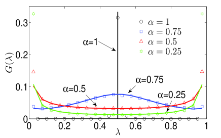
Figure 1: The PDF of the occupation fraction in half-space for a particle in the box $\left[-1,1\right]$. CTRW trajectories were generated as explained in Appendix B, with $x_{0}=0$. For each trajectory, the total time in $x>0$, $T_{+}$, was recorded, and the occupation fraction, $\lambda=T_{+}/t$, was calculated. The figure shows the PDF for long times of the occupation fraction $\lambda$ for $\alpha=1,0.75,0.5,0.25$ (symbols). Lamperti’s PDF, Eq. (43), is plotted as lines (For $\alpha=1$, the PDF for the simulations and the theory was scaled by 3 for visibility). While for $\alpha=1$, $\lambda$ is very narrowly distributed around $1/2$, for $\alpha<1$, the PDF becomes wider and even attains a U shape for small enough $\alpha$.

IV.1.2 An application of the occupation time functional— the first passage time PDF

As a side note, we demonstrate how the fractional Feynman-Kac equation for the occupation time can be applied in an elegant manner to the problem of the first passage time (FPT). The FPT in the box $\left[-\frac{L}{2},\frac{L}{2}\right]$ is defined as the time $t_{f}$ it takes a particle starting at $x_{0}=-b\;(0<b<L/2)$ to reach $x=0$ for the first time Redner_book . A relation between the occupation time functional of the previous subsection and the FPT was proposed by Kac Kac1951 :

$$\textrm{Pr}\{t_{f}>t\}=\textrm{Pr}\{\max_{0\leq\tau\leq t}x(\tau)<0\}=\lim_{p\rightarrow\infty}G_{x_{0}}(p,t),$$

where as in the previous subsection, $G_{x_{0}}(p,s)$ is the PDF of $T_{+}=\int_{0}^{t}\Theta[x(\tau)]d\tau$. The last equation is true since $G_{x_{0}}(p,t)=\int_{0}^{\infty}e^{-pT_{+}}G_{x_{0}}(T_{+},t)dT_{+}$, and thus, if the particle has never crossed $x=0$, we have $T_{+}=0$ and $e^{-pT_{+}}=1$, while otherwise, $T_{+}>0$ and for $p\rightarrow\infty$, $e^{-pT_{+}}=0$. Substituting $x_{0}=-b$ and $p\rightarrow\infty$ in Eq. (40) of the previous subsection gives

$$\lim_{p\rightarrow\infty}G_{-b}(p,s)=\frac{1}{s}\left\{1-\frac{\cosh\left[\left(\frac{L}{2}-b\right)\frac{s^{\alpha/2}}{\sqrt{K_{\alpha}}}\right]}{\cosh\left(\frac{Ls^{\alpha/2}}{2\sqrt{K_{\alpha}}}\right)}\right\}.$$ (45)

The first passage time PDF satisfies $f(t)=\frac{\partial}{\partial t}\left[1-\textrm{Pr}\{t_{f}>t\}\right]$. We therefore have in Laplace space,

$$f(s)=\frac{\cosh\left[\left(\frac{L}{2}-b\right)\frac{s^{\alpha/2}}{\sqrt{K_{\alpha}}}\right]}{\cosh\left(\frac{Ls^{\alpha/2}}{2\sqrt{K_{\alpha}}}\right)}.$$

For long times, the small $s$ limit gives

$$f(s)\approx 1-\frac{b(L-b)}{2K_{\alpha}}s^{\alpha}.$$

For $0<\alpha<1$, inverting $s\rightarrow t$,

$$f(t_{f})\approx\frac{b(L-b)}{2K_{\alpha}|\Gamma(-\alpha)|}t_{f}^{-(1+\alpha)}.$$ (46)

Therefore, $f(t_{f})\sim t_{f}^{-(1+\alpha)}$ (compared to $f(t_{f})\sim t_{f}^{-(1+\alpha/2)}$ for a free particle BarkaiPRE01 ; BarkaiJSP10 ), indicating that for $\alpha<1$, $\left\langle t_{f}\right\rangle=\infty$. Eqs. (45) and (46) agree with previous work BarkaiJSP06 ; BarkaiPRE06 .

IV.1.3 The fluctuations

Eq. (41), giving $G_{0}(p,s)$ for the occupation time functional, cannot be directly inverted. It can nevertheless be used to calculate the first few moments using

$$\left\langle T_{+}^{n}\right\rangle=(-1)^{n}\left.\frac{\partial^{n}}{\partial p^{n}}G_{0}(p,t)\right|_{p=0}.$$

The first moment (for $x_{0}=0$) is of course $\left\langle T_{+}\right\rangle=t/2$ or $\left\langle\lambda\right\rangle=1/2$. For the second moment,

$$\left\langle T_{+}^{2}\right\rangle_{s}=\frac{4-\alpha}{4s^{3}}-\frac{\alpha(s\tau)^{\alpha/2}}{2s^{3}\sinh\left[2(s\tau)^{\alpha/2}\right]}.$$ (47)

The long times, we take the limit of small $s$,

$$\left\langle T_{+}^{2}\right\rangle_{s}\approx\frac{2-\alpha}{2s^{3}}+\frac{\alpha\tau^{\alpha}}{6s^{3-\alpha}}.$$

Inverting and dividing by $t^{2}$, we obtain the fluctuations of the occupation fraction, $\left\langle(\Delta\lambda)^{2}\right\rangle=\left\langle\lambda^{2}\right\rangle-\left\langle\lambda\right\rangle^{2}$,

$$\left\langle(\Delta\lambda)^{2}\right\rangle\approx\frac{1-\alpha}{4}+\frac{\alpha}{6\Gamma(3-\alpha)}\left(\frac{t}{\tau}\right)^{-\alpha}.$$ (48)

For $\alpha<1$ and $t\rightarrow\infty$, we see from Eq. (48) that $\left\langle(\Delta\lambda)^{2}\right\rangle=\frac{1-\alpha}{4}>0$. For $\alpha=1$, $\left\langle(\Delta\lambda)^{2}\right\rangle\rightarrow 0$ as $t\rightarrow\infty$. The convergence to the long-times limit exhibits a $t^{-\alpha}$ decay. For $x_{0}\neq 0$, the first moment approaches $1/2$ as $\left\langle\lambda\right\rangle\approx 1/2+\frac{x_{0}(L-|x_{0}|)}{4K_{\alpha}\Gamma(2-\alpha)}t^{-\alpha}$ and the fluctuations remain the same as in Eq. (48) up to order $t^{-\alpha}$.

For short times (and $x_{0}=0$), taking the limit $(s\tau)^{\alpha/2}\gg 1$ in Eq. (47) gives $\left\langle T_{+}^{2}\right\rangle_{s}\approx\frac{4-\alpha}{4s^{3}}$, from which

$$\left\langle(\Delta\lambda)^{2}\right\rangle\approx\frac{1-\alpha/2}{4}.$$ (49)

This is the expected result, since for short times the PDF is Lamperti’s with index $\alpha/2$ (Eq. (44)).

The fluctuations $\left\langle(\Delta\lambda)^{2}\right\rangle$ are plotted in Figure 2 and agree well with Eq. (49) for short times and with Eq. (48) for long times. As expected, the approach to the asymptotic limit is slower as $\alpha$ becomes smaller.

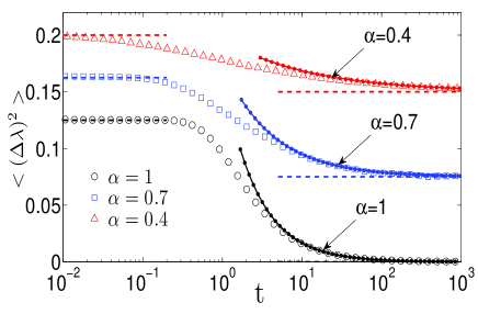
Figure 2: The fluctuations of the occupation fraction in half box. CTRW trajectories were generated as explained in Appendix B (with $x_{0}=0$) and the occupation fraction in half box, $\lambda=T_{+}/t$, was calculated. The figure shows the fluctuations $\left\langle(\Delta\lambda)^{2}\right\rangle$ vs. $t$ for $\alpha=0.4,0.7,1$ (symbols). Theory for long times, Eq. (48), is plotted as dotted lines. The fluctuations are initially equal to their free particle counterpart, $(1-\alpha/2)/4$ (Eq. (49), indicated as dashed lines), and then decay to their asymptotic value, $(1-\alpha)/4$ (also indicated as dashed lines), as $t^{-\alpha}$. Only for $\alpha=1$, the fluctuations vanish for $t\rightarrow\infty$.

IV.2 The time-averaged position in a harmonic potential

We consider the time-averaged position, $\overline{x}=\frac{1}{t}\int_{0}^{t}x(\tau)d\tau$, for a sub-diffusing particle in a harmonic potential, $V(x)=m\omega^{2}x^{2}/2$ (fractional Ornstein-Uhlenbeck process BarkaiPRL99 ; BarkaiJPC00 ).

IV.2.1 The distribution

We first study the PDF in the long-times limit using the general equation (38). Define the second moment in thermal equilibrium as $\left\langle x^{2}\right\rangle_{\textrm{th}}=k_{B}T/(m\omega^{2})$. Measuring $\overline{x}$ in units of $\sqrt{\left\langle x^{2}\right\rangle_{\textrm{th}}}$, we have for $t\rightarrow\infty$,

$$G(\overline{x})=\frac{1}{\sqrt{\left\langle x^{2}\right\rangle_{\textrm{th}}}}g\left(\frac{\overline{x}}{\sqrt{\left\langle x^{2}\right\rangle_{\textrm{th}}}}\right),$$

where

$$g(y)=\frac{\sin(\pi\alpha)}{\pi}\frac{I_{\alpha-1}^{<}(y)I_{\alpha}^{>}(y)+I_{\alpha-1}^{>}(y)I_{\alpha}^{<}(y)}{[I_{\alpha}^{>}(y)]^{2}+[I_{\alpha}^{<}(y)]^{2}+2\cos(\pi\alpha)I_{\alpha}^{>}(y)I_{\alpha}^{<}(y)},$$ (50)

with

$$I_{\alpha}^{<}=\int_{y}^{\infty}e^{-\frac{x^{2}}{2}}(x-y)^{\alpha}dx\;;\;I_{\alpha}^{>}=\int_{-\infty}^{y}e^{-\frac{x^{2}}{2}}(y-x)^{\alpha}dx.$$

Using Mathematica, we could express the solution of the integrals in Eq. (50) in terms of Kummer’s functions. The full expression is given in Appendix C (Eq. (Appendix C: The $t\rightarrow\infty$ distribution of the time-averaged position in a harmonic potential.)). It can be shown that for $\alpha=1$, $G(\overline{x})=\delta(\overline{x})$, as expected for an ergodic system BarkaiPRL07 ; BarkaiJSP08 . For $\alpha<1$, $G(\overline{x})$ has a non-zero width, and when $\alpha\rightarrow 0$, $G(\overline{x})=\sqrt{\frac{m\omega^{2}}{2\pi k_{B}T}}\exp\left[-\frac{m\omega^{2}\overline{x}^{2}}{2k_{B}T}\right]$, which is the Boltzmann distribution, since for $\alpha\rightarrow 0$, $\overline{x}\rightarrow x$ BarkaiPRL07 ; BarkaiJSP08 . For $\overline{x}\ll\sqrt{\left\langle x^{2}\right\rangle_{\textrm{th}}}$ ($y\ll 1$), $g(y)$ has a Taylor expansion around $y=0$ of the form $g(y)=\frac{\Gamma\left(\frac{\alpha}{2}\right)\tan\left(\frac{\pi\alpha}{2}\right)}{\sqrt{2}\pi\Gamma\left(\frac{1+\alpha}{2}\right)}+{\cal O}(y^{2})$. For $\overline{x}\gg\sqrt{\left\langle x^{2}\right\rangle_{\textrm{th}}}$ ($y\gg 1$), $g(y)\sim\frac{\Gamma(\alpha)\sin(\pi\alpha)}{\sqrt{2\pi^{3}}}y^{-2\alpha}e^{-y^{2}/2}$, which gives the expected results for $\alpha\rightarrow 0$ and $\alpha=1$. Eq. (50) is plotted and compared to simulations in Fig 3.

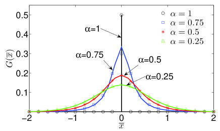
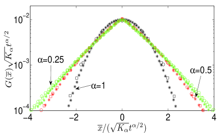
Figure 3: The PDF $G(\overline{x})$ for a particle in a binding harmonic field. CTRW trajectories were generated using the method described in Appendix B, with $x_{0}=0$. Top panel: Simulation results for long times for $\alpha=0.25,0.5,0.75,1$ (symbols). Theory for $t\rightarrow\infty$, Eq. (50), is plotted as solid lines (For $\alpha=1$, the PDF for the simulations and the theory was scaled by 2 for visibility). For $\alpha=1$, the distribution is a delta function, whereas for $\alpha<1$, $\overline{x}$ is a random variable even for long times, indicating ergodicity breaking. Bottom panel: Simulation results for the PDF of $\overline{x}$ for a number of short times and for $\alpha=0.25,0.5,1$ (symbols). The plot illustrates the free-particle scaling form, Eq. (51).

For short times, $t^{\alpha}\ll\left\langle x^{2}\right\rangle_{\textrm{th}}/K_{\alpha}$, the particle is at the minimum of the potential and therefore behaves as a free particle. For the free-particle case, we have previously shown a scaling form for $x_{0}=0$ BarkaiJSP10

$$G(\overline{x},t)=\frac{1}{\sqrt{K_{\alpha}}t^{\alpha/2}}h_{\alpha}\left(\frac{\overline{x}}{\sqrt{K_{\alpha}}t^{\alpha/2}}\right),$$ (51)

where $h_{\alpha}(y)$ is a dimensionless scaling function. This behavior is numerically demonstrated in Fig 3.

IV.2.2 The fluctuations

The PDF of the time-averaged position was shown in the previous subsection to have a non-trivial limiting distributions for $t\rightarrow\infty$ (Eq. (50)) and $t\rightarrow 0$ (Eq. (51)). However, the shape of the PDF for other times is unknown. In this subsection, we show that using the fractional Feynman-Kac equation, we can determine the width of the distribution for all times.

Let us write the forward equation in $(p,s)$ space for the functional $A=\overline{x}t=\int_{0}^{t}x(\tau)d\tau$ ($U(x)=x$) and for $x_{0}=0$. Since $A$ is not necessarily positive, $p$ here is the Fourier pair of $A$ and we use Eq. (28) of Section II.1.3:

$$sG(x,p,s)-\delta(x)=ipxG(x,p,s)$$ (52)

$$+K_{\alpha}\left[\frac{\partial^{2}}{\partial x^{2}}+\frac{\partial}{\partial x}\frac{m\omega^{2}x}{k_{B}T}\right][s-ipx]^{1-\alpha}G(x,p,s).$$

To find $\left\langle A^{2}\right\rangle$, we use the relation

$$\left\langle A^{2}\right\rangle_{s}=-\int_{-\infty}^{\infty}\left.\frac{\partial^{2}}{\partial p^{2}}G(x,p,s)\right|_{p=0}dx.$$

Operating on both sides of Eq. (52) with $-\frac{\partial^{2}}{\partial p^{2}}$, substituting $p=0$, and integrating over all $x$, we obtain, in $s$ space,

$$s\left\langle A^{2}\right\rangle_{s}=2\left\langle Ax\right\rangle_{s},$$ (53)

where we used the fact that the integral over the Fokker-Planck operator vanishes. Eq. (53) can be intuitively understood by noting that $\frac{\partial}{\partial t}\left\langle A^{2}\right\rangle=2\left\langle A\dot{A}\right\rangle$ and $\dot{A}=x$. We next use Eq. (52) and

$$\left\langle Ax\right\rangle_{s}=-i\int_{-\infty}^{\infty}x\left.\frac{\partial}{\partial p}G(x,p,s)\right|_{p=0}dx,$$

to obtain,

$$s\left\langle Ax\right\rangle_{s}=\left[1+(1-\alpha)(s\tau)^{-\alpha}\right]\left\langle x^{2}\right\rangle_{s}-s(s\tau)^{-\alpha}\left\langle Ax\right\rangle_{s},$$

where we defined the relaxation time $\tau^{\alpha}=k_{B}T/(K_{\alpha}m\omega^{2})=\left\langle x^{2}\right\rangle_{\textrm{th}}/K_{\alpha}$. Thus,

$$s\left\langle A_{x}x\right\rangle_{s}=\frac{(1-\alpha)+(s\tau)^{\alpha}}{1+(s\tau)^{\alpha}}\left\langle x^{2}\right\rangle_{s}.$$ (54)

Finally, to find $\left\langle x^{2}\right\rangle_{s}$, we use $\left\langle x^{2}\right\rangle_{s}=\int_{-\infty}^{\infty}x^{2}G(x,p=0,s)dx$,

$$s\left\langle x^{2}\right\rangle_{s}=2K_{\alpha}s^{-\alpha}-2s(s\tau)^{-\alpha}\left\langle x^{2}\right\rangle_{s},$$

where we used the normalization condition $\int G(x,p=0,s)dx=1/s$. Thus,

$$s\left\langle x^{2}\right\rangle_{s}=\frac{2\left\langle x^{2}\right\rangle_{\textrm{th}}}{2+(s\tau)^{\alpha}}.$$ (55)

Combining Eqs. (53), (54), and (55), we find,

$$\left\langle A^{2}\right\rangle_{s}=\frac{4}{s^{3}}\frac{(1-\alpha)+(s\tau)^{\alpha}}{1+(s\tau)^{\alpha}}\frac{\left\langle x^{2}\right\rangle_{\textrm{th}}}{2+(s\tau)^{\alpha}}.$$

To invert to the time domain, we write $\left\langle A^{2}\right\rangle_{s}$ as partial fractions:

$$\left\langle A^{2}\right\rangle_{s}=\frac{2\left\langle x^{2}\right\rangle_{\textrm{th}}}{s^{3}}\times$$ (56)

$$\left[(1-\alpha)+2\alpha\frac{(s\tau)^{\alpha}}{1+(s\tau)^{\alpha}}-(1+\alpha)\frac{(s\tau)^{\alpha}}{2+(s\tau)^{\alpha}}\right].$$

Inverting the last equation, we find

$$\left\langle A^{2}\right\rangle=\left\langle x^{2}\right\rangle_{\textrm{th}}t^{2}\times$$ (57)

$$\left\{(1-\alpha)+4\alpha E_{\alpha,3}\left[-(t/\tau)^{\alpha}\right]-2(1+\alpha)E_{\alpha,3}\left[-2(t/\tau)^{\alpha}\right]\right\},$$

where we used the Laplace transform relation Podlubny

$$\int_{0}^{\infty}e^{-st}t^{2}E_{\alpha,3}\left[-c(t/\tau)^{\alpha}\right]dt=\frac{1}{s^{3}}\frac{(s\tau)^{\alpha}}{c+(s\tau)^{\alpha}},$$

and $E_{\alpha,3}(z)$ is the Mittag-Leffler function, defined as Podlubny

$$E_{\alpha,3}(z)=\sum_{n=0}^{\infty}\frac{z^{n}}{\Gamma(3+\alpha n)}.$$

To obtain the fluctuations of the time-averaged position, $\left\langle(\Delta\overline{x})^{2}\right\rangle=\left\langle\overline{x}^{2}\right\rangle-\left\langle\overline{x}\right\rangle^{2}$, we use $\left\langle\overline{x}^{2}\right\rangle=\left\langle A^{2}\right\rangle/t^{2}$ and $\left\langle\overline{x}\right\rangle=0$ (since $x_{0}=0$). This gives

$$\left\langle(\Delta\overline{x})^{2}\right\rangle=\left\langle x^{2}\right\rangle_{\textrm{th}}\times$$ (58)

$$\left\{(1-\alpha)+4\alpha E_{\alpha,3}\left[-(t/\tau)^{\alpha}\right]-2(1+\alpha)E_{\alpha,3}\left[-2(t/\tau)^{\alpha}\right]\right\}.$$

Eq. (58) is plotted (using PodlubnyMLF ) and compared to simulations in the top panel of Figure 4.

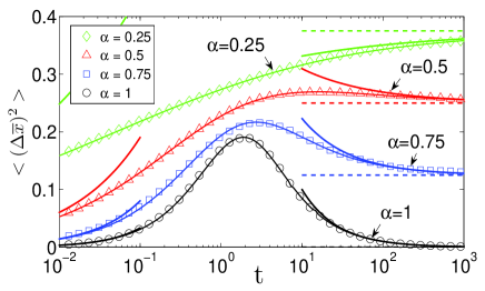
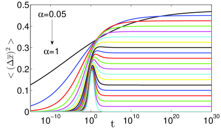
Figure 4: The fluctuations $\left\langle(\Delta\overline{x})^{2}\right\rangle$ for a particle in a harmonic potential. Top panel: CTRW trajectories were generated using the method described in Appendix B, with $x_{0}=0$. Symbols represent simulation results for $\alpha=0.25,0.5,0.75,1$. Theory, Eq. (58), is plotted as solid lines. The straight dashed lines are $\lim_{t\rightarrow\infty}\left\langle(\Delta\overline{x})^{2}\right\rangle=(1-\alpha)\left\langle x^{2}\right\rangle_{\textrm{th}}$. Except for $\alpha=1$, the fluctuations do not vanish when $t\rightarrow\infty$ and thus ergodicity is broken. The dotted lines represent the long-times and short-times approximations, Eqs. (59) and (60), respectively. Bottom panel: The fluctuations, Eq. (58), plotted for a wide time range $[10^{-15},10^{30}]$. Shown are 20 curves for $\alpha=0.05,0.1,0.15,...,1$ (top to bottom). The fluctuations display a maximum when $\alpha<1/3$ and a crossover when $\alpha\lesssim 0.15$. As expected, the fluctuations approach their asymptotic value slower for smaller values of $\alpha$.

To find the long times behavior of the fluctuations (58), we expand Eq. (56) for small $s$, invert, and divide by $t^{2}$,

$$\left\langle(\Delta\overline{x})^{2}\right\rangle\approx(1-\alpha)\left\langle x^{2}\right\rangle_{\textrm{th}}+\frac{(3\alpha-1)\left\langle x^{2}\right\rangle_{\textrm{th}}}{\Gamma(3-\alpha)}\left(\frac{t}{\tau}\right)^{-\alpha}.$$ (59)

Thus, for $\alpha<1$ and $t\rightarrow\infty$, $\left\langle(\Delta\overline{x})^{2}\right\rangle=(1-\alpha)\left\langle x^{2}\right\rangle_{\textrm{th}}>0$ and ergodicity is broken. Only when $\alpha=1$, we have ergodic behavior $\left\langle(\Delta\overline{x})^{2}\right\rangle=0$. As we observed for the occupation fraction (Eq. (48)), Eq. (59) too exhibits a $t^{-\alpha}$ convergence of the fluctuations to their asymptotic limit.

For short times,

$$E_{\alpha,3}\left[-(t/\tau)^{\alpha}\right]\approx\frac{1}{2}-\frac{(t/\tau)^{\alpha}}{\Gamma(3+\alpha)}.$$

Therefore,

$$\left\langle(\Delta\overline{x})^{2}\right\rangle\approx\frac{4\left\langle x^{2}\right\rangle_{\textrm{th}}}{\Gamma(3+\alpha)}\left(\frac{t}{\tau}\right)^{\alpha}.$$ (60)

Noting that $\left\langle x^{2}\right\rangle_{\textrm{th}}/\tau^{\alpha}=K_{\alpha}$, we can rewrite Eq. (60), as $\left\langle(\Delta\overline{x})^{2}\right\rangle\approx\frac{4K_{\alpha}}{\Gamma(3+\alpha)}t^{\alpha}$, which is, as expected, equal to the free particle expression BarkaiJSP10 .

The bottom panel of Figure 4 presents the fluctuations of the time-average (for $x_{0}=0$) for a wide range of times and for $\alpha=0.05,0.1,0.15,...,1$. As expected from Eqs. (59) and (60), the fluctuations increase from $\left\langle(\Delta\overline{x})^{2}\right\rangle=0$ at $t\rightarrow 0$ to their asymptotic value at $t\rightarrow\infty$, $\left\langle x^{2}\right\rangle_{\textrm{th}}(1-\alpha)$. However, as can be seen also in Eq. (59), for $\alpha>1/3$ the fluctuations display a maximum and decay to their asymptotic limit from above. We found numerically that the value of the maximal fluctuations scales roughly as $\alpha^{-1/2}$ (not shown). It can also be seen that for almost all times and all values of $\alpha$, the fluctuations $\left\langle(\Delta\overline{x})^{2}\right\rangle$ decrease as the diffusion becomes more “normal” (increasing $\alpha$), as expected. However, this pattern surprisingly breaks down for $\alpha\lesssim 0.15$, for which there is a time window when the fluctuations increase with $\alpha$.

It is straightforward to generalize our results to any initial condition with first moment $\left\langle x_{0}\right\rangle$ and second moment $\left\langle x_{0}^{2}\right\rangle$. The first moment of the time-average is $\left\langle\overline{x}\right\rangle=\left\langle x_{0}\right\rangle E_{\alpha,2}\left[-(t/\tau)^{\alpha}\right]$, which decays for long-times as $\left\langle\overline{x}\right\rangle\sim\frac{\left\langle x_{0}\right\rangle}{\Gamma(2-\alpha)}\left(\frac{t}{\tau}\right)^{-\alpha}$. The second moment is

$$\left\langle\overline{x}^{2}\right\rangle=(1-\alpha)\left\langle x^{2}\right\rangle_{\textrm{th}}+2\alpha\left[2\left\langle x^{2}\right\rangle_{\textrm{th}}-\left\langle x_{0}^{2}\right\rangle\right]E_{\alpha,3}\left[-(t/\tau)^{\alpha}\right]$$

$$+2(1+\alpha)\left[\left\langle x_{0}^{2}\right\rangle-\left\langle x^{2}\right\rangle_{\textrm{th}}\right]E_{\alpha,3}\left[-2(t/\tau)^{\alpha}\right],$$ (61)

from which the fluctuations directly follow. For long times,

$$\left\langle(\Delta\overline{x})^{2}\right\rangle \approx(1-\alpha)\left\langle x^{2}\right\rangle_{\textrm{th}}$$

$$+\frac{(3\alpha-1)\left\langle x^{2}\right\rangle_{\textrm{th}}+(1-\alpha)\left\langle x_{0}^{2}\right\rangle}{\Gamma(3-\alpha)}\left(\frac{t}{\tau}\right)^{-\alpha}.$$

For short times,

$$\left\langle(\Delta\overline{x})^{2}\right\rangle\approx\left\langle(\Delta x_{0})^{2}\right\rangle-2\left[\frac{\left\langle(\Delta x_{0})^{2}\right\rangle}{\Gamma(2+\alpha)}-\frac{2\left\langle x^{2}\right\rangle_{\textrm{th}}}{\Gamma(3+\alpha)}\right]\left(\frac{t}{\tau}\right)^{\alpha},$$

where $\left\langle(\Delta x_{0})^{2}\right\rangle=\left\langle x_{0}^{2}\right\rangle-\left\langle x_{0}\right\rangle^{2}$. According to the last two equations, if the system is already in equilibrium at $t=0$ such that $\left\langle x_{0}^{2}\right\rangle=\left\langle x^{2}\right\rangle_{\textrm{th}}$, the fluctuations monotonically decay, for all $\alpha$, from $\left\langle x^{2}\right\rangle_{\textrm{th}}$ at $t=0$ to $\left\langle x^{2}\right\rangle_{\textrm{th}}(1-\alpha)$ at $t\rightarrow\infty$.

For $\alpha=1$ (and $x_{0}=0$), we find the known result Risken :

$$\left\langle(\Delta\overline{x})^{2}\right\rangle_{\alpha=1}=\left(\frac{\tau}{t}\right)^{2}\left(4e^{-t/\tau}-e^{-2t/\tau}+\frac{2t}{\tau}-3\right).$$ (62)

To derive the last equation, we used the relation $E_{1,3}(z)=[e^{z}-z-1]/z^{2}$. Since the ordinary ($\alpha=1$) Ornstein-Uhlenbeck process is a Gaussian process VanKampen , the PDF of $\overline{x}$ is a Gaussian too, with the variance indicated by Eq. (62).

IV.2.3 Fractional Kramers equation

Finally, we remark on the connection between the fractional Feynman-Kac equation of this subsection and an important class of processes in which the velocity of the particle is the quantity undergoing sub-diffusion. For such processes, Friedrich and coworkers have recently developed a fractional Kramers equation for the joint position-velocity PDF FriedrichPRL06 ; FriedrichPRE06 . For example, consider a Rayleigh-like model in which a free, heavy test particle of mass $M$ collides with light bath particles at random times, but where the times between collisions are distributed according to $\psi(\tau)\sim\tau^{-(1+\alpha)}$. The PDF of the velocity of the test particle, $G(v,t)$, satisfies the fractional Fokker-Planck equation BarkaiJPC00 :

$$\frac{\partial}{\partial t}G(v,t)=\gamma_{\alpha}\left[\frac{k_{B}T}{M}\frac{\partial^{2}}{\partial v^{2}}+\frac{\partial}{\partial v}v\right]{\cal D}_{\textrm{RL},t}^{1-\alpha}G(v,t),$$

where ${\cal D}_{\textrm{RL},t}^{1-\alpha}$ is the Riemann-Liouville fractional derivative operator (see Section II.1.3) and $\gamma_{\alpha}$ is the damping coefficient. Since in the collisions model $x(t)=\int_{0}^{t}v(\tau)d\tau$, $x$ is a functional of the trajectory $v(\tau)$, and therefore, the joint PDF of $x$ and $v$, $G(v,x,t)$, is described by our fractional Feynman-Kac equation. Denoting the Fourier transform $x\rightarrow p$ of $G(v,x,t)$ as $G(v,p,t)$, we have (see Eq. (28)),

$$\frac{\partial}{\partial t}G(v,p,t) =ipvG(v,p,t)$$ (63)

$$+\gamma_{\alpha}\left[\frac{k_{B}T}{M}\frac{\partial^{2}}{\partial v^{2}}+\frac{\partial}{\partial v}v\right]{\cal D}_{t}^{1-\alpha}G(v,p,t),$$

where ${\cal D}_{t}^{1-\alpha}$ is the fractional substantial derivative, here equal in Laplace $s$ space to $(s-ipv)^{1-\alpha}$. Within this model, for $0<\alpha<1$ the motion is ballistic, $\left\langle x^{2}\right\rangle\sim t^{2}$, while for $\alpha=1$ it is diffusive, $\left\langle x^{2}\right\rangle\sim t$ (see Eq. (59)). Eq. (63) is exactly equal to the fractional Kramers equation derived by Friedrich and coworkers FriedrichPRL06 ; FriedrichPRE06 , and in that sense, our results generalize their pioneering work.

V Summary and discussion

Time-averages of sub-diffusive continuous-time random walks (CTRW) in binding fields are known to exhibit weak ergodicity breaking and were thus the subject of recent interest. In this paper, we used the Feynman-Kac approach to develop a general equation for time-averages of CTRW (Eq. (22)), which can be seen as a fractional generalization of the Feynman-Kac equation for Brownian motion. The equation we derived describes the distribution of time-averages for all observables, potentials, and times. We also derived a backward equation (Eq. (31)) which is useful in practical problems.

We investigated two applications of our equations: the occupation fraction in the positive half of a box, and the time-averaged position in a harmonic potential. In both cases, we obtained expressions for the PDF for long times and for short times and calculated the fluctuations. We found that the fluctuations decay as $t^{-\alpha}$ to their asymptotic limit, which is non-zero for anomalous diffusion, $\alpha<1$. Our fractional Feynman-Kac equation thus provides a general tool for the treatment of time-averages and for the study of the kinetics of weak ergodicity breaking.

Recently, the occupation time functional has been studied in the context of dynamical systems with an infinite (non-normalizable) invariant measure Zweimuller . It remains to be seen whether a framework similar to that of the fractional Feynman-Kac equation could be developed for general functionals of these processes. We also note that while the (integer) Feynman-Kac equation can be derived using path integrals MajumdarReview , a path integral approach for functionals of anomalous sub-diffusion is still awaiting (but see preliminary results in the upcoming book FractionalDynamicsBook ).

Appendix A: Time-dependent forces

In our model of CTRW with a time-dependent force, jump probabilities are determined according to the force at the time of the jump. To derive an equation for $G(x,A,t)$ in that case, we rewrite Eq. (7) as follows:

$$\chi(x,A,t)=G_{0}(x)\delta(A)\delta(t)$$ (64)

$$+\int_{0}^{t}\psi(\tau)L(x+a,t)\chi[x+a,A-\tau U(x+a),t-\tau]d\tau$$

$$+\int_{0}^{t}\psi(\tau)R(x-a,t)\chi[x-a,A-\tau U(x-a),t-\tau]d\tau.$$

Note that the jump probabilities are time-dependent (but have no memory). Laplace transforming $A\rightarrow p$ and $t\rightarrow s$, using the Laplace identity ${\cal L}\{tf(t)\}=-\frac{\partial}{\partial s}f(s)$,

$$\chi(x,p,s)=G_{0}(x)$$

$$+L\left(x+a,-\frac{\partial}{\partial s}\right)\hat{\psi}[s+pU(x+a)]\chi(x+a,p,s)$$

$$+R\left(x-a,-\frac{\partial}{\partial s}\right)\hat{\psi}[s+pU(x-a)]\chi(x-a,p,s).$$

Fourier transforming $x\rightarrow k$,

$$\chi(k,p,s)=\hat{G}_{0}(k)+ \left[\cos(ka)+i\sin(ka)\frac{aF\left(-i\frac{\partial}{\partial k},-\frac{\partial}{\partial s}\right)}{2k_{B}T}\right]\times$$

$$\hat{\psi}\left[s+pU\left(-i\frac{\partial}{\partial k}\right)\right]\chi(k,p,s).$$

Continuing as in Section II.1.2, we find the formal solutions for $\chi(k,p,s)$ and $G(k,p,s)$ and then take the continuum limit. This gives:

$$sG(k,p,s)-\hat{G}_{0}(k)=-pU\left(-i\frac{\partial}{\partial k}\right)G(k,p,s)$$

$$-K_{\alpha}\left[k^{2}-ik\frac{F\left(-i\frac{\partial}{\partial k},-\frac{\partial}{\partial s}\right)}{k_{B}T}\right]\times$$

$$\left[s+pU\left(-i\frac{\partial}{\partial k}\right)\right]^{1-\alpha}G(k,p,s).$$

Inverting $k\rightarrow x,s\rightarrow t$, we obtain the fractional Feynman-Kac equation for a time-dependent force:

$$\frac{\partial}{\partial t}G(x,p,t)=K_{\alpha}{\cal L}^{\textrm{(t)}}_{\textrm{FP}}{\cal D}_{t}^{1-\alpha}G(x,p,t)-pU(x)G(x,p,t),$$ (65)

where

$${\cal L}^{\textrm{(t)}}_{\textrm{FP}}=\frac{\partial^{2}}{\partial x^{2}}-\frac{\partial}{\partial x}\frac{F(x,t)}{k_{B}T}$$

is the time-dependent Fokker-Planck operator.

Appendix B: The simulation method

The fractional Feynman-Kac equation describes the joint PDF of $x$ and $A$ in the continuum limit of CTRW. In this limit, $a\rightarrow 0$ and $B_{\alpha}\rightarrow 0$ but the generalized diffusion coefficient $K_{\alpha}=a^{2}/(2B_{\alpha})$ (Eq. (21)) is kept finite BarkaiPRE00 . We simulate trajectories of this process as follows HanggiSimulations . We place a particle on a one-dimensional lattice in initial position $x_{0}$, where usually $x_{0}=0$. We set the lattice spacing $a$ and the generalized diffusion coefficient $K_{\alpha}$ and determine $B_{\alpha}=a^{2}/(2K_{\alpha})$. Waiting times are then drawn for $\alpha=1$ from an exponential distribution $\psi(\tau)=e^{-\tau/\tau_{0}}/\tau_{0}$ with mean $\tau_{0}=B_{1}$. This is implemented by setting $\tau=-\tau_{0}\ln(u)$, where $u$ is a number uniformly distributed in $[0,1]$. For $\alpha<1$, we set $\tau_{0}=[B_{\alpha}/\Gamma(1-\alpha)]^{1/\alpha}$ and $\tau=\tau_{0}u^{-1/\alpha}$, which corresponds to $\psi(\tau)=\frac{B_{\alpha}}{|\Gamma(-\alpha)|}\tau^{-(1+\alpha)}$ ($\tau\geq\tau_{0}$; see Eq. (5)). After waiting time $\tau$, we move the particle right or left with probabilities $R(x)$ or $L(x)$, respectively, as given by Eq. (14). For the harmonic potential, Eq. (14) gives $R(x)=\frac{1}{2}\left(1-\frac{ax}{2\left\langle x^{2}\right\rangle_{\textrm{th}}}\right)$ and $L(x)=\frac{1}{2}\left(1+\frac{ax}{2\left\langle x^{2}\right\rangle_{\textrm{th}}}\right)$. Since the typical $x$ is of the order of $\sqrt{\left\langle x^{2}\right\rangle_{\textrm{th}}}$, it is sufficient to choose $a\ll\sqrt{\left\langle x^{2}\right\rangle_{\textrm{th}}}$ to guarantee that $0<R(x),L(x)<1$ (see discussion in BarkaiPRE06 ). For the box, $R(x)=L(x)=1/2$ and we make the boundaries at $x=\pm\frac{L}{2}$ reflecting.

The parameters we used in the simulations were as follows. In all simulations, we used $a=0.1$ or smaller, and each curve represents at least $10^{4}$ trajectories. For the occupation time in a box, we set $L=2$ and $K_{\alpha}=1$, and the final simulation time in Figure 1 was $t=10^{3}$. For the time-averaged position in the harmonic potential, we set $K_{\alpha}=1/2$ and $\left\langle x^{2}\right\rangle_{\textrm{th}}=1/2$ (or $\tau^{\alpha}=1$). In Figure 3, the final simulation times were as follows. For the long-times limit (top panel) we used $t=10^{7},10^{4},10^{3},10^{3}$ for $\alpha=0.25,0.5,0.75,1$, respectively. For the short times (bottom panel), we used $t=10^{-3},10^{-2},10^{-1}$ for $\alpha=1$, $t=10^{-5},10^{-4},10^{-3}$ for $\alpha=0.5$, and $t=10^{-6},10^{-5},10^{-4}$ for $\alpha=0.25$.

Appendix C: The $t\rightarrow\infty$ distribution of the time-averaged position in a harmonic potential.

Consider the time-averaged position, $\overline{x}=\frac{1}{t}\int_{0}^{t}x(\tau)d\tau$, for a sub-diffusing particle in a harmonic potential, $V(x)=m\omega^{2}x^{2}/2$. Using the thermal second moment, $\left\langle x^{2}\right\rangle_{\textrm{th}}=k_{B}T/(m\omega^{2})$, and for $t\rightarrow\infty$, we have

$$G(\overline{x})=\frac{1}{\sqrt{\left\langle x^{2}\right\rangle_{\textrm{th}}}}g\left(\frac{\overline{x}}{\sqrt{\left\langle x^{2}\right\rangle_{\textrm{th}}}}\right),$$

where

$$g(y)=\frac{\sin(\pi\alpha)}{\pi}\times$$

$$\left\{e^{y^{2}/2}y\Gamma\left(\frac{\alpha}{2}\right)\Gamma(1+\alpha)\left[\text{M}\left(\frac{1-\alpha}{2},\frac{1}{2},-\frac{y^{2}}{2}\right)\text{U}\left(1+\frac{\alpha}{2},\frac{3}{2},\frac{y^{2}}{2}\right)+2\text{M}\left(\frac{1-\alpha}{2},\frac{3}{2},-\frac{y^{2}}{2}\right)\text{U}\left(\frac{\alpha}{2},\frac{1}{2},\frac{y^{2}}{2}\right)\right]\right.$$

$$\left.+\sqrt{2}\Gamma(\alpha)\Gamma\left(\frac{1+\alpha}{2}\right)\left[y^{2}\alpha\text{M}\left(\frac{1+\alpha}{2},\frac{3}{2},\frac{y^{2}}{2}\right)\text{U}\left(1+\frac{\alpha}{2},\frac{3}{2},\frac{y^{2}}{2}\right)+2\text{M}\left(\frac{1+\alpha}{2},\frac{1}{2},\frac{y^{2}}{2}\right)\text{U}\left(\frac{\alpha}{2},\frac{1}{2},\frac{y^{2}}{2}\right)\right]\right\}\times$$

$$\left\{2^{2+\alpha}y^{2}\Gamma^{2}\left(1+\frac{\alpha}{2}\right)\left[e^{y^{2}}\text{M}^{2}\left(\frac{1-\alpha}{2},\frac{3}{2},-\frac{y^{2}}{2}\right)-2\cos(\pi\alpha)\text{M}^{2}\left(1+\frac{\alpha}{2},\frac{3}{2},\frac{y^{2}}{2}\right)\right]\right.$$

$$+4\sqrt{2}e^{y^{2}}\sqrt{\pi}y\Gamma(1+\alpha)\text{M}\left(\frac{1-\alpha}{2},\frac{3}{2},-\frac{y^{2}}{2}\right)\text{M}\left(-\frac{\alpha}{2},\frac{1}{2},-\frac{y^{2}}{2}\right)$$

$$+2^{1+\alpha}\Gamma^{2}\left(\frac{1+\alpha}{2}\right)\left[e^{y^{2}}\text{M}^{2}\left(-\frac{\alpha}{2},\frac{1}{2},-\frac{y^{2}}{2}\right)+2\cos(\pi\alpha)\text{M}^{2}\left(\frac{1+\alpha}{2},\frac{1}{2},\frac{y^{2}}{2}\right)\right]$$

$$\left.+2^{-\alpha}y^{2}\Gamma^{2}(1+\alpha)\text{U}^{2}\left(1+\frac{\alpha}{2},\frac{3}{2},\frac{y^{2}}{2}\right)\right\}^{-1}.$$ (66)

In the last equation, $\text{M}(a,b,z)$ is the confluent hypergeometric (or Kummer’s) function of the first kind and $\text{U}(a,b,z)$ is the confluent hypergeometric (or Kummer’s) function of the second kind Abramowitz . Eq. (Appendix C: The $t\rightarrow\infty$ distribution of the time-averaged position in a harmonic potential.) is valid for $y>0$. Due to the symmetry of the potential, $g(-y)=g(y)$.

References

- [1] S. Havlin and D. ben-Avraham. Diffusion in disordered media. Adv. Phys., 36:695, 1987.
- [2] J. P. Bouchaud and A. Georges. Anomalous diffusion in disordered media: Statistical mechanisms, models and physical applications. Phys. Rep., 195:127, 1990.
- [3] R. Metzler and J. Klafter. The random walk’s guide to anomalous diffusion: A fractional dynamics approach. Phys. Rep., 339:1, 2000.
- [4] R. Klages, G. Radons, and I. M. Sokolov, editors. Anomalous Transport: Foundations and Applications. Wiley-VCH, Weinheim, 2008.
- [5] E. W. Montroll and G. H. Weiss. Random walks on lattices. II. J. Math. Phys., 6:167, 1965.
- [6] H. Scher and E. Montroll. Anomalous transit-time dispersion in amorphous solids. Phys. Rev. B, 12:2455, 1975.
- [7] G. Bel and E. Barkai. Weak ergodicity breaking in the continuous-time random walk. Phys. Rev. Lett., 94:240602, 2005.
- [8] E. Barkai. Residence time statistics for normal and fractional diffusion in a force field. J. Stat. Phys., 123:883, 2006.
- [9] A. Rebenshtok and E. Barkai. Distribution of time-averaged observables for weak ergodicity breaking. Phys. Rev. Lett., 99:210601, 2007.
- [10] A. Rebenshtok and E. Barkai. Weakly non-ergodic statistical physics. J. Stat. Phys., 133:565, 2008.
- [11] J. P. Bouchaud. Weak ergodicity breaking and aging in disordered systems. J. de Physique I, 2:1705, 1992.
- [12] D. S. Grebenkov. Residence times and other functionals of reflected Brownian motion. Phys. Rev. E, 76:041139, 2007.
- [13] S. N. Majumdar and A. Comtet. Local and occupation time of a particle diffusing in a random medium. Phys. Rev. Lett., 89:060601, 2002.
- [14] G. Zumofen, J. Hohlbein, and C. G. Hübner. Recurrence and photon statistics in fluorescence fluctuation spectroscopy. Phys. Rev. Lett., 93:260601, 2004.
- [15] N. Agmon. The residence time equation. Chem. Phys. Lett., 497:184, 2010.
- [16] I. Y. Wong, M. L. Gardel, D. R. Reichman, E. R. Weeks, M. T. Valentine, A. R. Bausch, and D. A. Weitz. Anomalous diffusion probes microstructure dynamics of entangled F-actin networks. Phys. Rev. Lett., 92:178101, 2004.
- [17] G. Pesce, L. Selvaggi, A. Caporali, A. C. De Luca, A. Puppo, G. Rusciano, and A Sasso. Mechanical changes of living oocytes at maturation investigated by multiple particle tracking. Appl. Phys. Lett., 95:093702, 2009.
- [18] G. G. Cabal, A. Genovesio, S. Rodriguez-Navarro, C. Zimmer, O. Gadal, A. Lesne, H. Buc, F. Feuerbach-Fournier, J.-C. Olivo-Marin, E. C. Hurt, and U. Nehrbass. SAGA interacting factors confine sub-diffusion of transcribed genes to the nuclear envelope. Nature, 441:770, 2006.
- [19] I. Bronstein, Y. Israel, E. Kepten, S. Mai, Y. Shav-Tal, E. Barkai, and Y. Garini. Transient anomalous diffusion of telomeres in the nucleus of mammalian cells. Phys. Rev. Lett., 103:018102, 2009.
- [20] I. Golding and E. C. Cox. Physical nature of bacterial cytoplasm. Phys. Rev. Lett., 96:098102, 2006.
- [21] I. M. Tolić-Nørrelykke, E.-L. Munteanu, G. Thon, L. Oddershede, and K. Berg-Sørensen. Anomalous diffusion in living yeast cells. Phys. Rev. Lett., 93:078102, 2004.
- [22] S. N. Majumdar. Brownian functionals in physics and computer science. Curr. Sci., 89:2076, 2005.
- [23] M. Kac. On distributions of certain Wiener functionals. Trans. Am. Math. Soc., 65:1, 1949.
- [24] L. Turgeman, S. Carmi, and E. Barkai. Fractional Feynman-Kac equation for non-Brownian functionals. Phys. Rev. Lett., 103:190201, 2009.
- [25] S. Carmi, L. Turgeman, and E. Barkai. On distributions of functionals of anomalous diffusion paths. J. Stat. Phys., 141:1071, 2010.
- [26] R. Friedrich, F. Jenko, A. Baule, and S. Eule. Anomalous diffusion of inertial, weakly damped particles. Phys. Rev. Lett., 96:230601, 2006.
- [27] R. Friedrich, F. Jenko, A. Baule, and S. Eule. Exact solution of a generalized Kramers-Fokker-Planck equation retaining retardation effects. Phys. Rev. E, 74:041103, 2006.
- [28] E. Barkai, R. Metzler, and J. Klafter. From continuous time random walks to the fractional Fokker-Planck equation. Phys. Rev. E, 61:132, 2000.
- [29] T. Miyaguchi and T. Akimoto. Ultraslow convergence to ergodicity in transient subdiffusion. Phys. Rev. E, 83:062101, 2011.
- [30] I. M. Sokolov and R. Metzler. Towards deterministic equations for Lévy walks: The fractional material derivative. Phys. Rev. E, 67:010101(R), 2003.
- [31] R. Metzler, E. Barkai, and J. Klafter. Anomalous diffusion and relaxation close to thermal equilibrium: A fractional Fokker-Planck equation approach. Phys. Rev. Lett., 82:3563, 1999.
- [32] E. Barkai. Fractional Fokker-Planck equation, solution, and application. Phys. Rev. E, 63:046118, 2001.
- [33] I. M. Sokolov and J. Klafter. Field-induced dispersion in subdiffusion. Phys. Rev. Lett., 97:140602, 2006.
- [34] E. Heinsalu, M. Patriarca, I. Goychuk, and P. Hänggi. Use and abuse of a fractional Fokker-Planck dynamics for time-dependent driving. Phys. Rev. Lett., 99:120602, 2007.
- [35] M. Magdziarz and A. Weron. Equivalence of the fractional Fokker-Planck and subordinated Langevin equations: The case of a time-dependent force. Phys. Rev. Lett., 101:210601, 2008.
- [36] B. I. Henry, T. A. M. Langlands, and P. Straka. Fractional Fokker-Planck equations for subdiffusion with space- and time-dependent forces. Phys. Rev. Lett., 105:170602, 2010.
- [37] S. Eule and R. Friedrich. Subordinated Langevin equations for anomalous diffusion in external potentials— Biasing and decoupled external forces. EPL, 86:30008, 2009.
- [38] C. Godrèche and J. M. Luck. Statistics of the occupation time of renewal processes. J. Stat. Phys., 104:489, 2001.
- [39] J. Lamperti. An occupation time theorem for a class of stochastic processes. Trans. Am. Math. Soc., 88:380, 1958.
- [40] G. Margolin and E. Barkai. Non-ergodicity of a time series obeying Lévy statistics. J. Stat. Phys., 122:137, 2006.
- [41] S. Redner. A Guide to First-Passage Processes. Cambridge University Press, 2001.
- [42] M. Kac. On some connections between probability theory and differential and integral equations. In Second Berkeley Symposium on Mathematical Statistics and Probability, page 189, Berkeley, CA, USA, 1951. University of California Press.
- [43] G. Bel and E. Barkai. Random walk to a nonergodic equilibrium concept. Phys. Rev. E, 73:016125, 2006.
- [44] E. Barkai and R. J. Silbey. Fractional Kramers equation. J. Phys. Chem. B, 104:3866, 2000.
- [45] I. Podlubny. Fractional Differential Equations. Academic Press, New York, 1999.
- [46] I. Podlubny. http://www.mathworks.com/matlabcentral, 2009.
- [47] H. Risken. The Fokker Planck Equation: Methods of Solution and Applications. Springer, 2nd edition, 1989.
- [48] N. G. Van Kampen. Stochastic Processes in Physics and Chemistry. North Holland, 3rd edition, 2007.
- [49] M. Thaler and R. Zweimüller. Distributional limit theorems in infinite ergodic theory. Probab. Theory Rel., 135:15, 2006.
- [50] Fractional dynamics: Recent advances. 2011.
- [51] E. Heinsalu, M. Patriarca, I. Goychuk, G. Schmid, and P. Hänggi. Fractional Fokker-Planck dynamics: Numerical algorithm and simulations. Phys. Rev. E, 73:046133, 2006.
- [52] M. Abramowitz and I. A. Stegun, editors. Handbook of Mathematical Functions with Formulas, Graphs, and Mathematical Tables. Dover Publications, New York, 1972.