Reference analysis of the signal + background model in counting experiments

Abstract

The model representing two independent Poisson processes, labelled as “signal” and “background” and both contributing additively to the total number of counted events, is considered from a Bayesian point of view. This is a widely used model for the searches of rare or exotic events in presence of a background source, as for example in the searches performed by high-energy physics experiments. In the assumption of prior knowledge about the background yield, a reference prior is obtained for the signal alone and its properties are studied. Finally, the properties of the full solution, the marginal reference posterior, are illustrated with few examples.

1 Introduction

Searches for rare events or faint signals are very common in scientific research. Here we consider only counting experiments, as for example underground detectors which measure the result of high-energy particle collisions, and we are interested in situations in which a known set of “background” processes contributes to the number of observed events, on top of which one looks for a possible excess which can be attributed to the faint signal. In these situations, most searches do not find evidences for a new signal and their results are summarized by providing upper limits to the signal intensity (see for example [1]). The analysis of the significance of an experimental result or of the expected significance of a planned measurement is a very important task, and the problem has been treated several times in the frequentist framework (see for example [2, 3]). Here the problem is approached from the Bayesian point of view, as it has been recently done by Demortier, Jain, and Prosper in Ref. [4] (hereafter named the “DJP paper”), whose work stimulated the present study and a similar paper by Pierini, Prosper, Sekmen and Spiropulu al. [5] (hereafter named the “PPSS paper”)

We assume that the integer number $k=0,1,\ldots$ of observed events follows a Poisson distribution and that the signal and background sources are independently Poisson distributed with parameters $s$ and $b$, such that the probability to observe $k$ counts comes from a Poisson distribution with parameter $s+b$: $P(k)=\text{Poi}(k|s+b)$. Here we are interested in the signal intensity $s\geq 0$, as it is practically always the case in the searches for new phenomena, and treat $b\geq 0$ as a nuisance parameter.

In the Bayesian framework, the result of the statistical inference is provided by the joint posterior probability density

$$p(s,b|k)\propto\text{Poi}(k|s+b)\,p(s,b)$$ (1)

where $p(s,b)$ is the prior density which encodes the experimenter’s degree of belief before incorporating the results of the experiment with the information available before performing the experiment, and the likelihood function is the Poisson model $\text{Poi}(k|s+b)$ itself, considered as a function of $s+b$ for $k$ fixed at the actual observation. The normalization constant can be found by imposing that the integral of $p(s,b|k)$ is one.

Here we look for a solution which only depends on the assumed model and the observed data, but not on any additional prior information, hence choose to follow the approach dictated by the so-called reference analysis [6]. A key ingredient is the formulation of the reference prior $\pi(s,b)$ [7], defined as to maximize the amount of missing information, and the result of the inference is the reference posterior obtained by using $\pi(s,b)$ in place of $p(s,b)$ in the Bayes’ theorem (1). Because we are not interested in making inference about $b$, we integrate the posterior over it to obtain the marginal posterior $p(s|k)=\int_{0}^{\infty}p(s,b|k)\,\text{d}b$, our final solution. This approach has been followed also by the DJP and PPSS papers.

Although DJP considered signal and background as independent Poisson processes as in this work, they preferred a model in which the signal strength is multiplied by a parameter which should encode the uncertainty about both the signal efficiency and the integrated luminosity. However, the background parameter is not multiplied by a similar quantity, although one expects to have some luminosity dependent factor here too. A better model would describe the probability of counting $n$ events as the Poisson probability $\text{Poi}(n|(\varepsilon_{s}\sigma+\varepsilon_{b}\mu)\mathcal{L})$ in which the signal cross-section $\sigma$ is multiplied by the signal efficiency $\varepsilon_{s}$, the background cross-section $\mu$ is multiplied by the corresponding efficiency $\varepsilon_{b}$, and the integrated luminosity $\mathcal{L}$ explicitly appears, because it affects the same way signal and background yields (being 100% correlated). Such model would be quite complex: $\sigma$ is the only parameter of interest, hence the marginal posterior is obtained after the integration over the remaining four nuisance parameters. The prior for $\mu$ would be a Gamma density as in the DJP paper (the Gamma density is the conjugate prior for the Poisson process), the priors for the efficiencies $\varepsilon_{s},\varepsilon_{b}$ would be Beta densities (the conjugate family for the binomial problem), and the prior for $\mathcal{L}$ would be a Gaussian (or a Gamma density peaked very far from zero, looking very similar to a Gaussian). For the purpose of the present work, this model is too complicated. To simplify things, we treat a model in which there are only two parameters $s,b$ describing the expected numbers of events coming from the signal and background processes, assumed to be mutually independent (and independent from other parameters which do not appear explicitly in the model, like the luminosity, as it is done in the PPSS paper).

Here $s$ and $b$ are dimensionless numbers (not cross-sections) which are sufficient to describe in a stylized way the “discovery problem” in which one is interested in finding an excess of events over the background prediction. Qualitatively, in case a statistically significant excess is found, the next step is to evaluate the signal cross-section which corresponds to the measurement, which requires adopting the complicated model above, with a single parameter of interest and four nuisance parameters. Although in practice one works since the very beginning with a very complex model (with several parameters modelling the detector response and the theoretical uncertainties), from the mathematical point of view discovery and cross-section measurements can be considered two distinct phases, which can be treated in sequence. Here we consider the statistical approach which is sufficient for the discovery problem in a counting experiment for which the total uncertainty on the background yield is the only nuisance parameter, and defer the treatment of the complex model which is needed for estimating the cross-section to another paper.

In this paper we do not address in details the general Bayesian approach to discovery, but focus only on the marginal posterior for the signal in presence of backgrond with unknown yield (which is a necessary but not sufficient ingredient). However, the Reader should be aware that there are several issues in the use of the “Bayes’ factor” when taking a decision among two or more possible hypotheses when improper priors are used, as recently summarized by Berger [8]. The widespread use of flat priors in Bayesian computations basically makes it impossible to take a decision based on the Bayes factor in a proper way, and this is true also for the reference prior in the Poisson model considered here (see below), which is improper. Instead, the two posterior solutions which correspond to the competing hypotheses should be compared. This approach has no hidden trap when improper priors are chosen, and the only difficulty is that there is no consensus about the threshold which the posterior ratio should exceed to claim a discovery, contrasting with the conventional frequentist “five-sigma” rule for the significance of the discrepancy with respect to the background-only hypothesis (which is not free of problems [9]). A promising formal approach based on the Bayesian decision theory is being proposed by Bernardo [10], which is based on decision theory. One would choose the hypothesis which minimizes the expected posterior loss incurring when acting as if that hypothesis were correct. A convenient choice of a loss function which is parametrization invariant is the so-called “intrinsic discrepancy loss”, defined as the minimum among the two Kullback-Leibler directed divergences between two probability models [11]. When averaged over the reference posterior, the reference posterior intrinsic loss has a scale which can be mapped onto the displacement with respect to the Gaussian mean. This way, a threshold which corresponds to the “five-sigma” rule, or any other minimal significance, can be defined. For more details, see [10] and the papers cited therein.

In all searches for new phenomena there is quite a lot of information about the background, coming from several auxiliary measurements plus Monte Carlo simulations of the known physical processes. If this were not true, nobody would trust a discovery of a new signal based on the outcome of the experiment. Hence we assume that an informative prior for $b$ is available which encodes the experimenter’s degree of belief about the “reasonable” range of $b$ and its “most likely” values, written in the form of a Gamma density (the conjugate prior of the Poisson model):

$$p(b)=\text{Ga}(b|\alpha,\beta)=\frac{\beta^{\alpha}}{\Gamma(\alpha)}\,b^{\alpha-1}\,e^{-\beta b}$$ (2)

with shape parameter $\alpha>0$ and rate parameter $\beta>0$ (or scale parameter $\theta=1/\beta>0$). In the simple (but frequent) case in which there is limited prior knowledge about $b$ and only its expectation and variance are known, the Gamma parameters are determined by imposing $E[b]=\alpha/\beta$ and $V[b]=\alpha/\beta^{2}$.

Incidentally, one can note that it is quite common to use a Gaussian distribution to model the uncertainty on the yield of the background processes, although strictly speaking this is not the correct solution. The reason is that the density function should be defined on the domain of the parameter, which in this case is $b\in\mathbb{R}^{+}$, whereas the Gaussian distribution is defined over the whole real axis. Hence, the normal distribution needs to be truncated at zero, which implies renormalizing it and recomputing its mean and standard deviation (when $\text{N}(x;\mu,\sigma)$ is truncated at zero, $\mu$ remains the peak position but is no more equal to the mean, and $\sigma$ is related to the right-width but is no more the standard deviation). When the distance (in units of $\sigma$) between the peak and the origin is big enough, in practice one can proceed as if no truncation were necessary. However, this is often not the case, such that truncation does need to be considered. Because the domain of a random variable is the very first ingredient in the specification of a probability model, it appears more reasonable to limit the search for the background prior to the functions which are defined on the positive real semiaxis only. Two reasonable choices are the log-normal distribution and the Gamma density. The first may have a theoretical motivation when the uncertainty is attributed to the fluctuations of several additional independent contributions whose scale is uncertain. However, a Gamma density can mimic a log-normal distribution very well (and also a normal distribution when the latter is a good approximation) and has the advantage of belonging to the family of conjugate priors for the Poisson model, which implies that the posterior also belongs to the same family. This makes the choice of a conjugate prior most convenient, because simple relations exist between the parameters of the prior and posterior Gamma densities, which only depend on the observed data. It is worth emphasizing that this choice does not set any limit to the shape of the prior: a linear combination of Gamma densities can reproduce any shape. In this case, the posterior will be a linear combination, with the same weights, of the solutions which correspond to any individual Gamma density appearing in the prior, thanks to the linearity of the Bayes’ theorem (1).

Often, in particle-physics experiments the selection which is performed on the events has the goal of suppressing as much as possible the background contribution, while keeping a high efficiency for the signal. This often means that the background estimate has a sizable uncertainty, because the background events surviving the selection fall in the tails of the distributions of the physical observables, which would require the generation of enormous numbers of events to be well reproduced by Monte Carlo simulations. Hence the marginal prior density is often quite broad. In the opposite situation in which $b$ is perfectly known, the prior (2) degenerates in a $\delta$ function, which happens when $\alpha,\beta\to\infty$ while keeping $E[b]=\alpha/\beta=b_{0}$ constant (it is sufficient to set $\beta=\alpha/b_{0}$, which implies $V[b]=b_{0}/\alpha\to 0$). In this case, it is easy to show (appendix D) that the reference prior for $s$ is Jeffreys’ prior for $s^{\prime}=s+b_{0}$ (i.e. $b_{0}$ simply redefines the origin of the random variable): $\pi(s)\propto(s+b_{0})^{-1/2}$. In the following, we address the general problem with any value of $\alpha,\beta>0$.

Because no prior knowledge is assumed for the signal parameter $s$, a reference prior $\pi(s)$ for $s$ is desired, such that the joint prior can be written in the form $p(s,b)=p(s)\,p(b|s)=\pi(s)\,\text{Ga}(b|\alpha,\beta)$. Two techniques for finding the reference prior when the conditional density of the other parameter is known are explained by Sun and Berger [12], although only the second one (“Option 2” in their paper) is applied here. Such technique can be summarized as follows. The starting point is the marginal model $p(k|s)$, specifying the probability of counting $k\geq 0$ events in the hypothesis that the signal yield is $s\geq 0$ with the assumed knowledge about the background contribution:

$$p(k|s)=\int_{0}^{\infty}\text{Poi}(k|s+b)\,\text{Ga}(b|\alpha,\beta)\,\text{d}b\;.$$ (3)

Next, this model is used to compute the Fisher’s information

$$\begin{split}I(s)&=E\left[\left(\frac{\partial}{\partial s}\log p(k|s)\right)^{\!2\,}\right]\\ &=-E\left[\left(\frac{\partial^{2}}{\partial s^{2}}\log p(k|s)\right)\right]\end{split}$$ (4)

where the last expression is valid for asymptotically normal models, as in our case. Finally, the reference prior for $s$ is then $\pi(s)\propto|I(s)|^{1/2}$ [12].

In the rest of the paper, these steps are considered in sequence. Section 2 illustrates the properties of the marginal model $p(k|s)$, which is used in section 3 to compute the Fisher’s information $I(s)$. Finally, the reference prior $\pi(s)$ is computed in section 4 and few examples of its application are shown in section 5.

2 The marginal model

Here we find an explicit formula for the marginal model (3), in terms of the Poisson-Gamma mixture [13, 14]

$$\begin{split}P(k|\alpha,\beta)&=\int_{0}^{\infty}\text{Poi}(k|\theta)\,\text{Ga}(\theta|\alpha,\beta)\,\text{d}\theta\\ &=\frac{\beta^{\alpha}\,\Gamma(\alpha+k)}{k!\,\Gamma(\alpha)\,(1+\beta)^{\alpha+k}}\end{split}$$ (5)

a result which can be obtained by means of the Gamma integral

$$\Gamma(a)=\int_{0}^{\infty}x^{a-1}e^{-x}\,\text{d}x\;.$$

First, we note that

$$\begin{split}\text{Poi}(k|s+b)&=e^{-s-b}\,\frac{(s+b)^{k}}{k!}\\ &=\frac{e^{-s-b}}{k!}\sum_{n=0}^{k}\binom{k}{n}\,s^{k-n}\,b^{n}\\ &=e^{-s-b}\sum_{n=0}^{k}\frac{s^{k-n}\,b^{n}}{n!\,(k-n)!}\end{split}$$ (6)

which allows to rewrite (3) in the form

$$\begin{split}p(k|s)&=\sum_{n=0}^{k}\frac{e^{-s}\,s^{k-n}}{(k-n)!}\int_{0}^{\infty}\frac{b^{n}\,e^{-b}}{n!}\,\text{Ga}(b|\alpha,\beta)\,\text{d}b\\ &=\sum_{n=0}^{k}\frac{e^{-s}\,s^{k-n}}{(k-n)!}\int_{0}^{\infty}\text{Poi}(n|b)\,\text{Ga}(b|\alpha,\beta)\,\text{d}b\end{split}$$ (7)

which, with the help of (5), becomes

$$\begin{split}p(k|s)&=\left(\frac{\beta}{1+\beta}\right)^{\!\alpha}\sum_{n=0}^{k}\frac{\Gamma(n+\alpha)/\Gamma(\alpha)}{n!\,(1+\beta)^{n}}\,\frac{e^{-s}\,s^{k-n}}{(k-n)!}\\ &=\left(\frac{\beta}{1+\beta}\right)^{\!\alpha}\sum_{n=0}^{k}\frac{(\alpha)^{(n)}}{n!\,(1+\beta)^{n}}\,\text{Poi}(k-n|s)\;.\end{split}$$ (8)

The “rising factorial” (or Pochammer function) $(\alpha)^{(n)}=\Gamma(n+\alpha)/\Gamma(\alpha)=\alpha(\alpha+1)(\alpha+2)\cdots(\alpha+n-1)$ is defined as

$$(\alpha)^{(n)}=\begin{cases}1&\text{if}\;\,n=0\\ \alpha&\text{if}\;\,n=1\\ (\alpha)^{(k-1)}(\alpha+k-1)&\text{if}\;\,n=k>1\\ \end{cases}$$

and the ratio $(\alpha)^{(n)}/n!$ defines the binomial coefficient $\binom{\alpha+n-1}{n}$ with a upper real parameter, such that the the marginal model (8) can be also written in the final form

$$p(k|s)=\left(\frac{\beta}{1+\beta}\right)^{\!\alpha}e^{-s}\,f(s;k,\alpha,\beta)\;.$$ (9)

where the polynomial

$$f(s;k,\alpha,\beta)=\sum_{n=0}^{k}\binom{\alpha+n-1}{n}\frac{s^{k-n}}{(k-n)!\,(1+\beta)^{n}}$$ (10)

has explicit forms given in table 1.

The function $f(s;k,\alpha,\beta)$ has some interesting properties which are useful in the following treatment. The proofs are given in appendix B. Appendix A provides additional information which is useful when writing code to evaluate this polynomial.

Property 1.

For each $\alpha,\beta>0$ and $s\geq 0$ the series $\sum_{k=0}^{\infty}f(s;k,\alpha,\beta)$ converges to

$$\sum_{k=0}^{\infty}f(s;k,\alpha,\beta)=\left(\frac{1+\beta}{\beta}\right)^{\!\alpha}e^{s}\;.$$

This ensures that the the marginal model (9) is properly normalized.

Property 2.

The $n$-th partial derivative of $f(s;k,\alpha,\beta)$ with respect to $s$ is

$$f^{(n)}(s;k,\alpha,\beta)=\begin{cases}0&\text{if}\quad k<n\\ 1&\text{if}\quad k=n\\ f(s;k-n,\alpha,\beta)&\text{if}\quad k\geq n\\ \end{cases}$$ (11)

Property 2 makes it easy to compute all derivatives, the evaluation of a single function being sufficient.

Property 3.

For each finite $n\geq 1$, the sum $\sum_{k=0}^{\infty}f^{(n)}(s;k,\alpha,\beta)$ also converges to $e^{s}(1+\beta)^{\alpha}/\beta^{\alpha}$.

This ensures that the the expectation $E[f^{(n)}/f]=1$ for each $n$.

Figure 1: Marginal likelihood for different background priors, with 1 and 10 observed counts.

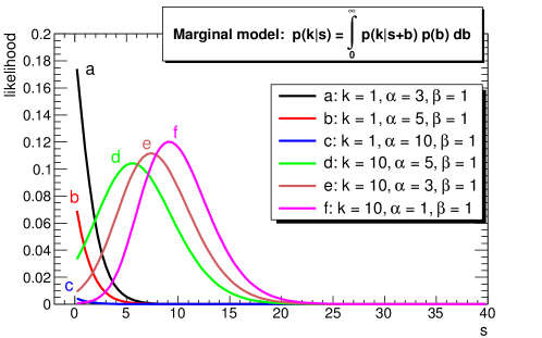
The marginal likelihood is shown in figure 1, for different background parameters, in the case of 1 and 10 observed counts. As shown in details in the appendix C, the marginal model (9) coincides with the appropriate limit of the marginal model of the DJP paper and with the marginal model of the PPSS paper.

$k$	$f(s;k,\alpha,\beta)$
0	1
1	$\displaystyle s+\frac{\alpha}{1+\beta}$
2	$\displaystyle\frac{s^{2}}{2}+\frac{s\,\alpha}{1+\beta}+\frac{\alpha(\alpha+1)}{2(1+\beta)^{2}}$
3	$\displaystyle\frac{s^{3}}{6}+\frac{s^{2}\alpha}{2(1+\beta)}+\frac{s\,\alpha(\alpha+1)}{2(1+\beta)^{2}}+\frac{\alpha(\alpha+1)(\alpha+2)}{6(1+\beta)^{3}}$
$n>4$	$\displaystyle\frac{s^{n}}{n!}+\frac{s^{n-1}}{(n-1)!}\frac{\alpha}{(1+\beta)}+\frac{s^{n-2}}{(n-2)!}\frac{\alpha(\alpha+1)}{2(1+\beta)^{2}}+\frac{s^{n-3}}{(n-3)!}\frac{\alpha(\alpha+1)(\alpha+2)}{3!\,(1+\beta)^{3}}+\cdots$
	$\displaystyle\cdots+\frac{\alpha(\alpha+1)\cdots(\alpha+n-1)}{n!\,(1+\beta)^{n}}$

Table 1: Explicit forms of $f(s;k,\alpha,\beta)$ for small values of $k$.

3 The Fisher’s information

The logarithm of the marginal model (9) is

$$\log p(k|s)=\alpha\log\frac{\beta}{1+\beta}-s+\log f(s;k,\alpha,\beta)$$ (12)

and its derivative with respect to $s$ is

$$\frac{\partial\log p(k|s)}{\partial s}=-1+\frac{f^{(1)}(s;k,\alpha,\beta)}{f(s;k,\alpha,\beta)}$$ (13)

while the second derivative is

$$\frac{\partial^{2}\log p(k|s)}{\partial s^{2}}=\frac{f^{(2)}(s;k,\alpha,\beta)}{f(s;k,\alpha,\beta)}-\left[\frac{f^{(1)}(s;k,\alpha,\beta)}{f(s;k,\alpha,\beta)}\right]^{2}$$ (14)

The expectation in the definition of the Fisher’s information (4) splits in two terms:

$$I(s)=E\left[\frac{[f^{(1)}(s;k,\alpha,\beta)]^{2}}{[f(s;k,\alpha,\beta)]^{2}}\right]-E\left[\frac{f^{(2)}(s;k,\alpha,\beta)}{f(s;k,\alpha,\beta)}\right]$$ (15)

which can be evaluated independently. The expectation $E[f^{(2)}/f]$ is one by virtue of Property 3.

The other term in (15) is

$$\begin{split}E\left[(f^{(1)}/f)^{2}\right]&=\left(\frac{\beta}{1+\beta}\right)^{\!\alpha}e^{-s}\,\sum_{k=0}^{\infty}\frac{[f^{(1)}(s;k,\alpha,\beta)]^{2}}{f(s;k,\alpha,\beta)}\\ \qquad\{k=0\Rightarrow&f^{(1)}=0\;\text{hence start from $k=1$; use Property 2}\}\\ &=\left(\frac{\beta}{1+\beta}\right)^{\!\alpha}e^{-s}\,\sum_{k=1}^{\infty}\frac{[f(s;k-1,\alpha,\beta)]^{2}}{f(s;k,\alpha,\beta)}\\ \qquad\{\text{now set}&\;n=k-1\}\\ &=\left(\frac{\beta}{1+\beta}\right)^{\!\alpha}e^{-s}\,\sum_{n=0}^{\infty}\frac{[f(s;n,\alpha,\beta)]^{2}}{f(s;n+1,\alpha,\beta)}\end{split}$$

which is easy to implement in a numerical routine, because one only needs a single evaluation of $f(s;k,\alpha,\beta)$ for each term in the sum (appendix A), in a loop which terminates when the current addendum gives a negligible contribution (for example, when the ratio between the addendum and the partial sum becomes less than $10^{-6}$, as it was done in the examples considered in the next section).

Finally, the Fisher’s information is

$$I(s)=\left(\frac{\beta}{1+\beta}\right)^{\!\alpha}e^{-s}\,\sum_{n=0}^{\infty}\frac{[f(s;n,\alpha,\beta)]^{2}}{f(s;n+1,\alpha,\beta)}-1$$ (16)

the same result being obtained when computing the expectation of the square of the first derivative (13) of the marginal log-likelihood, because $E[f^{(1)}/f]=1$ by virtue of Property 3. Appendix D shows that $I(s)$ gives the correct reference prior (Jeffreys’ prior) when there is certain prior knowledge about the background yield.

4 The reference prior

The reference prior for $s$ is $\pi(s)\propto|I(s)|^{1/2}$ [12]. From equation (16) one obtains

$$|I(s)|^{1/2}=\left|\left(\frac{\beta}{1+\beta}\right)^{\!\alpha}e^{-s}\,\sum_{n=0}^{\infty}\frac{[f(s;n,\alpha,\beta)]^{2}}{f(s;n+1,\alpha,\beta)}-1\right|^{1/2}$$ (17)

which only requires the evaluation of the function $f(s;n,\alpha,\beta)$ (see appendix A) to be computed once per cycle.

When $s\to\infty$ the function (17) is not decreasing fast enough to make it integrable over the positive real axis. In the asymptotic regime, the leading term in the polynomial $f(s;k,\alpha,\beta)$ is proportional to $s^{k}$, which means that each addendum in the sum diverges as a polynomial of degree $s^{n-1}$, and the exponential $e^{-s}$ is not sufficient to ensure that the sum goes to zero for $s\to\infty$ (easier to check in log scale: $\log(e^{-s}\,s^{n})=-s+n\log s\to\infty$ when both $n$ and $s$ go to $\infty$). This means that $\pi(s)$ is not a proper prior: it cannot represent somebody’s degree of belief. In the framework of the Bayesian reference analysis, the use of improper reference priors is admitted, provided that the reference posterior is a proper probability density (which is the case here).

For $s\to 0$ the polynomial $f(s;n,\alpha,\beta)$ reduces to a constant

$$\begin{split}f(0;n,\alpha,\beta)&=\binom{\alpha+n-1}{n}(1+\beta)^{-n}\\ &=\frac{\alpha+n-1}{n(1+\beta)}\,f(0;n-1,\alpha,\beta)\end{split}$$ (18)

which goes to zero for $n\to\infty$ fast enough to make the series in equation (17) converge. The function $|I(s)|^{1/2}$ has its single maximum at zero, hence a possible definition of the reference prior for the signal is

$$\pi(s)=\frac{|I(s)|^{1/2}}{|I(0)|^{1/2}}$$ (19)

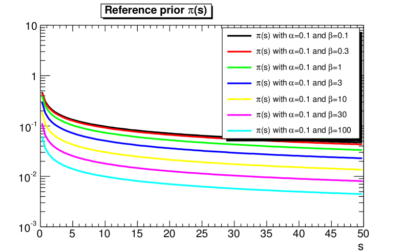
which is a monotonically decreasing function attaining its maximum value of one at zero. The reference prior $\pi(s)$ is shown in figure 2 for different choices of background parameters. The maximum at $s=0$ becomes more pronounced for small values of $\alpha$ and large values of $\beta$, whereas large values of $\alpha$ and small values of $\beta$ make the prior flat. As expected, combinations which have similar background expectation and variance give almost the same curve. In figure 2 such examples are: the $(\alpha,\beta)$ pairs $(0.1,3)$ and $(1,30)$, which have $E[b]=0.03$ and $E[b]=0.033$, both with $V[b]=0.011$; the pairs $(0.1,10)$ and $(1,100)$, both with $E[b]=0.01$, which have $V[b]=0.001$ and $V[b]=0.0001$; the pairs $(1,10)$ and $(10,100)$, both with $E[b]=0.1$, which have $V[b]=0.01$ and $V[b]=0.001$.

Figure 2: Reference prior for the signal parameter $s$ obtained with background parameters $\alpha=0.1$ (top-left), $\alpha=1$ (bottom-left), $\alpha=10$ (top-right) and $\beta=0.1,0.3,1,3,10,30,100$. The top-down sequence of the functions is the same as the list in the legend of each plot.

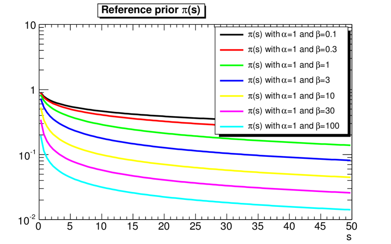
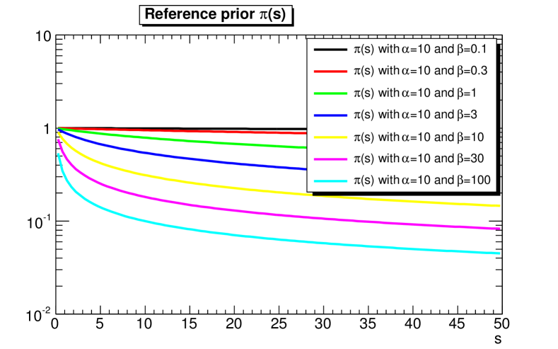
5 The marginal reference posterior

The joint prior for our model is the improper function $\pi(s,b)=\pi(s)\,p(b)$ where $\pi(s)$ is defined by equation (19) (or any other function which is proportional to $|I(s)|^{1/2}$) and $p(b)$ is the Gamma density (2) which encodes the experimenter’s prior degree of belief about the background.

The joint reference posterior is proportional to $p(s,b|k)\propto\text{Poi}(k|s+b)\,p(b)\,\pi(s)$ and the joint marginal posterior for $s$ is obtained after integration over $b$. Finally, because $\pi(s)$ does not explicitly depend on $b$, the marginal posterior is proportional to the product of the reference prior (19) and the marginal likelihood (9):

$$p(s|k)\propto\left(\frac{\beta}{1+\beta}\right)^{\!\alpha}e^{-s}\,f(s;k,\alpha,\beta)\,\pi(s)\;.$$ (20)

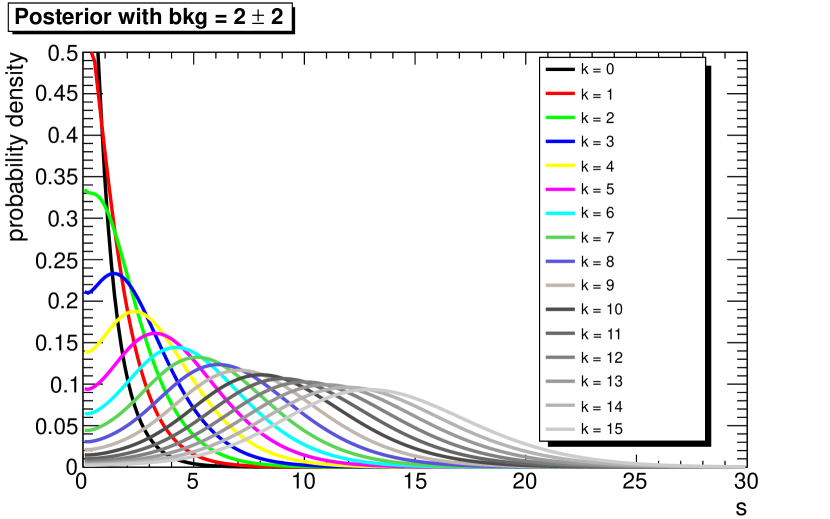
In order to illustrate the properties of the marginal reference posterior (20), we choose examples in which the prior expectation is small ($E[b]=2$) and the number of observed events is small too ($k=0,1,\ldots,15$ counts), and find the 68.3%, 90%, and 95% posterior credible intervals for the signal, choosing central intervals if they contain the posterior mode or upper limits otherwise (both are invariant under reparametrization). We consider uncertainties on the prior expectation of 10%, 20%, 50%, and 100%, such that the shape and rate parameters of the background prior are listed in table 4 and the corresponding prior densities are shown in figure 4. The marginal model, for different choices of the background prior and sample size, is shown in figure 5. The corresponding marginal posteriors are shown in figure 6, and their numerical summaries are provided by the tables 3, 4, 5 and 6 of appendix E, in the form of left and right bounds of the 68.3%, 90%, 95% credible intervals, mean, median, mode, variance, skewness and excess kurtosis.

$E[b]$	rel. unc.	$\alpha$	$\beta$
2	0.1	100	50.0
2	0.2	25	12.5
2	0.5	4	2.0
2	1.0	1	0.5

Figure 3: Parameters for the background priors.

Figure 4: The background prior distributions.

Figure 5: Marginal likelihood for the true signal, for different background priors ($E[b]=2$ with relative uncertainty 10%, 20%, 50%, and 100% from top-left to bottom-right) and sample sizes ($k=0,1,\ldots,15$).

Figure 6: Marginal posteriors for the signal, for different background priors ($E[b]=2$ with relative uncertainty 10%, 20%, 50%, and 100% from top-left to bottom-right) and sample sizes ($k=0,1,\ldots,15$).

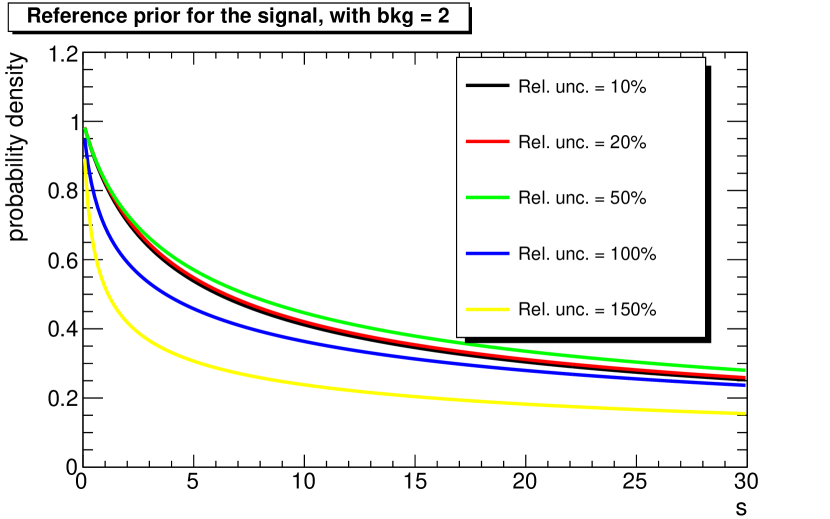
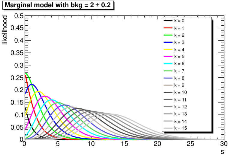
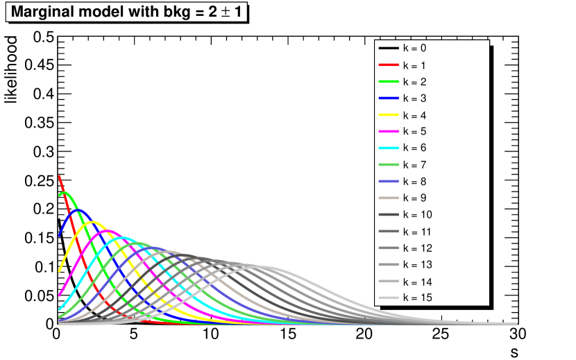
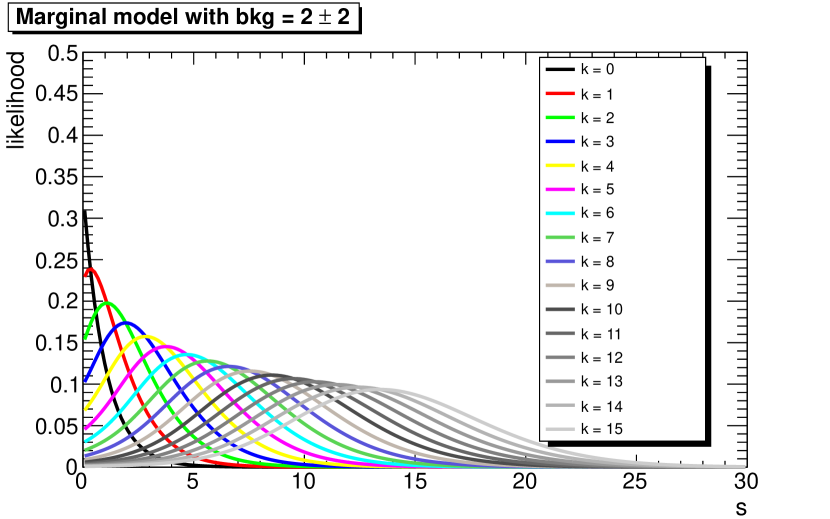
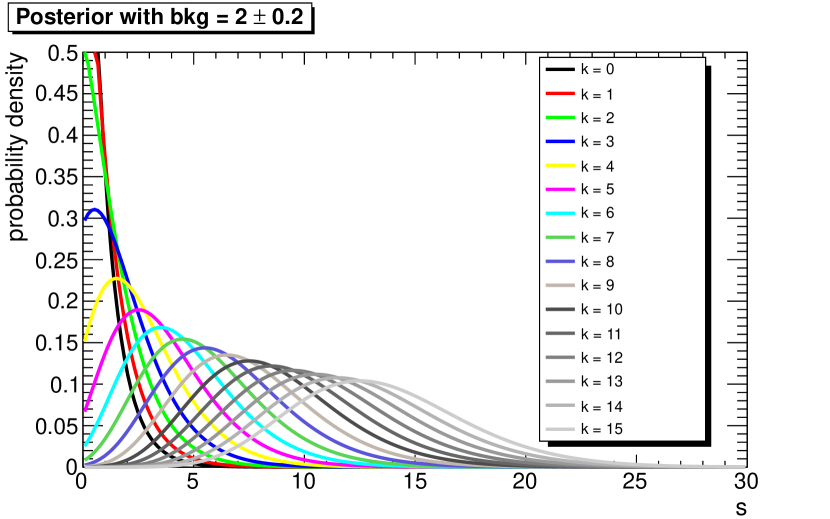
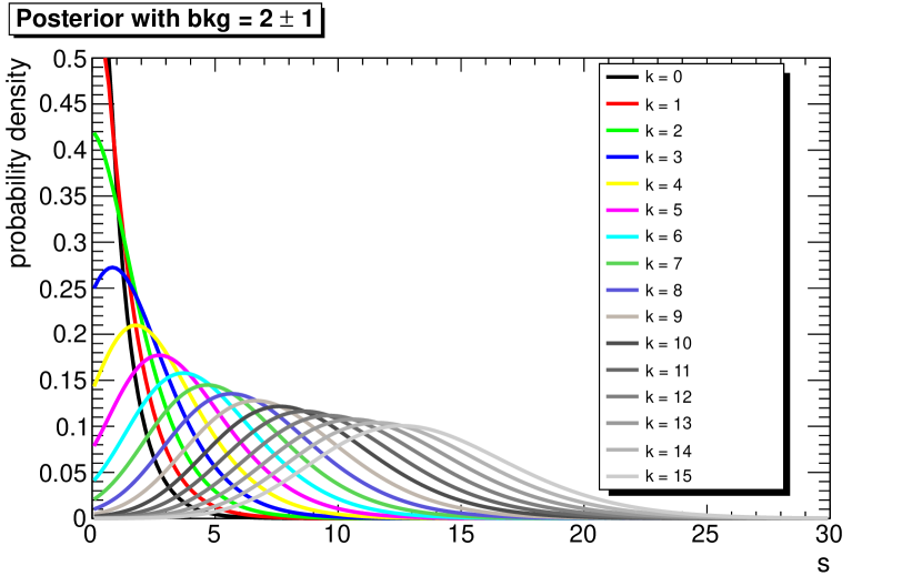
One aspect which deserves some comment is the case of zero observed counts. Although the marginal posterior (20) does not explicitly depends on the expected background, it still contains it indirectly, due to the integration over the background prior. This implies that the upper limit in case of no counted events (as for any counts) does depend on the background prior. This has been verified with a scan of the prior parameters, choosing a background expectation of $E[b]=0.5,1,2,4,8$ counts and a relative uncertainty of 10%, 20%, 50%, 100%, and 150%. The results are shown in table 2, which reports the posterior upper limit at 95% credibility level for zero counts as a function of the prior background expectation and relative uncertainty. The upper limit moves right with increasing background expectation, because the posterior becomes broader. On the other hand, it has a small increase (negligible if $E[b]$ is very small) for increasing relative uncertainties up to 50%, and then tends to decrease for increasing uncertainties, with a more pronounced trend for high background expectations.

Quoting upper limits which depend on the prior background expectation in the case of zero observed counts produces a result which is similar to the classical results (summarized in [15]) but may appear suboptimal from the Bayesian point of view. The reason is that one important piece of information is ignored: in this case we know with certainty that there is no contribution from the background process, hence one can interpret the result using the simpler model in which the signal alone is described by a Poisson process. Using the reference prior (which is Jeffreys’ prior) in this case gives the reference posterior $p(s|0)=Ga(s;\frac{1}{2},1)$ and the upper limit, found as the 0.95-quantile of the Gamma density, is 1.92 counts, which is lower than all values reported in table 2. One would obtain the same result with the model presented here, in the limit of a prior delta-function for the background prior which gives a unit mass to the single point $b=0$, because in this case one obtains the 1-dimensional Poisson model (by virtue of the result of appendix D). This upper limit does not depend on the prior knowledge about the background and looks a bit “aggressive”, compared to the well known upper limit of 3 counts which is obtained in the 1-dimensional case both using a flat prior (which is falsely considered non-informative and leads to solutions which are not invariant under reparametrization) and the classical approach [15]. On the other hand, it is the result of including all available information about the problem under consideration.

$E[b]$	Relative uncertainty on $E[b]$:
$\downarrow$	10%	20%	50%	100%	150%
0.5	2.55	2.55	2.56	2.57	2.55
1.0	2.65	2.66	2.68	2.66	2.60
2.0	2.77	2.78	2.80	2.74	2.62
4.0	2.88	2.89	2.91	2.78	2.62
8.0	2.96	2.98	2.99	2.81	2.62

Table 2: Upper limits at 95% credibility level for zero observed counts.

Given the observed counts and the prior beliefs on the background values, the method described in this paper provides an objective Bayesian solution for the statistical inference about the true signal, the marginal reference posterior (20). In the context of a specific analysis, it is important to study the sampling properties of the solution. In the large sample size limit, Bayesian $q$-credible regions are always approximate confidence regions with coverage $q$ and in some case they have even the exact coverage, as it happens for location-scale models [16]. However, the actual measurement may be far from the asymptotic regime. In addition our model is discrete, such that the coverage is not exact (of course this is also true for frequentist solutions), even though the fluctuations around the coverage $q$ become smaller and smaller with increasing sample sizes.

A frequentist study of the coverage for different solutions of the Poisson problem, in which the reference posterior (which corresponds to the use of the Jeffreys’ prior) is also included, is presented in Ref. [17]. We adopted a similar treatment to study few examples in which the small sample size is clearly far from the asymptotic limit, such that the coverage properties are not expected to be ideal. Different possible observations ($k=0,1,\ldots,15$ counts) have been considered. The coverage properties are a function of five parameters: the true signal and background yields, the shape and rate parameters of the background prior, and the observed count. The first step is to average over the possible observations with the corresponding Poisson weights, which leaves four degrees of freedom. We report the results obtained with the four background priors which correspond to an expectation of $E[b]=2$ with relative uncertainty of 10%, 20%, 50%, and 100% (the actual study considered background expectations of 0.5, 1, 2, 4, and 8 counts and also included the case of 5% and 150% relative uncertainties, but the qualitative features are the same as the examples presented here). For each prior, we still have two degrees of freedom left, the true signal and background yields. Hence the coverage can be shown in the form of 2-dimensional histograms.

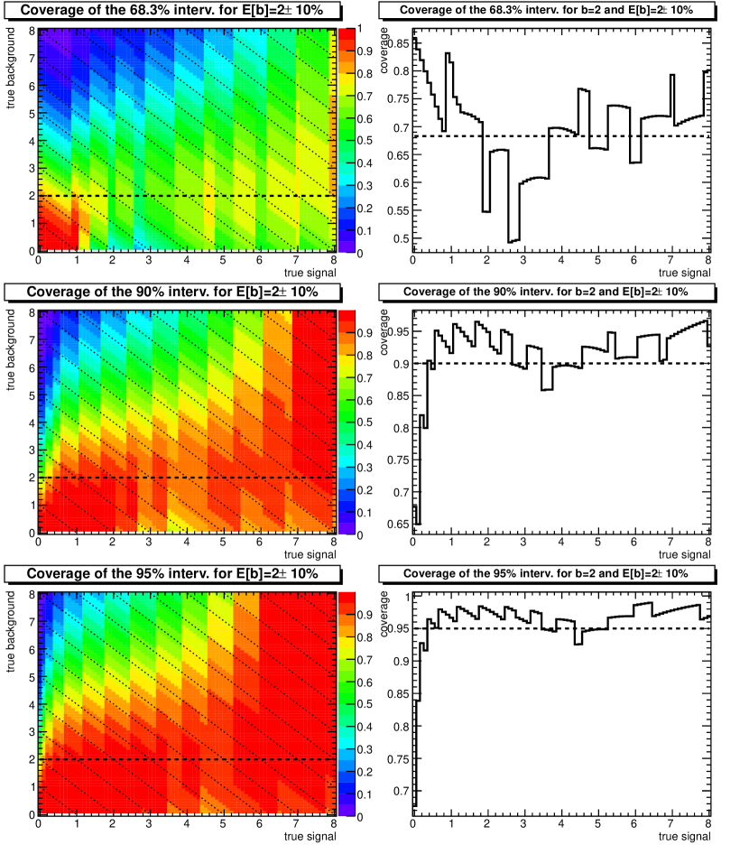
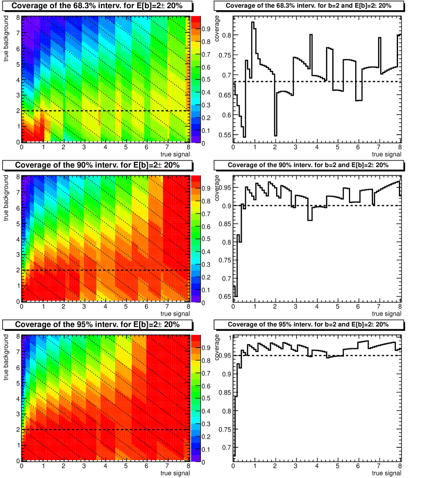
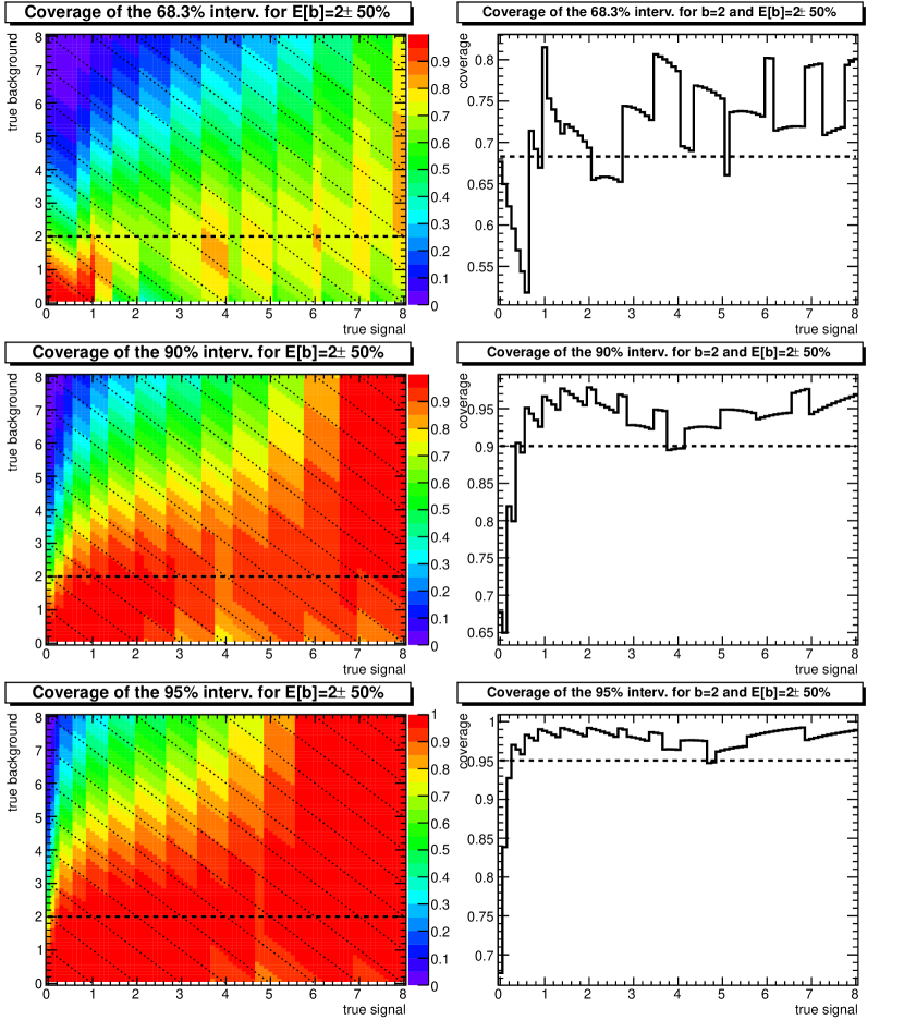
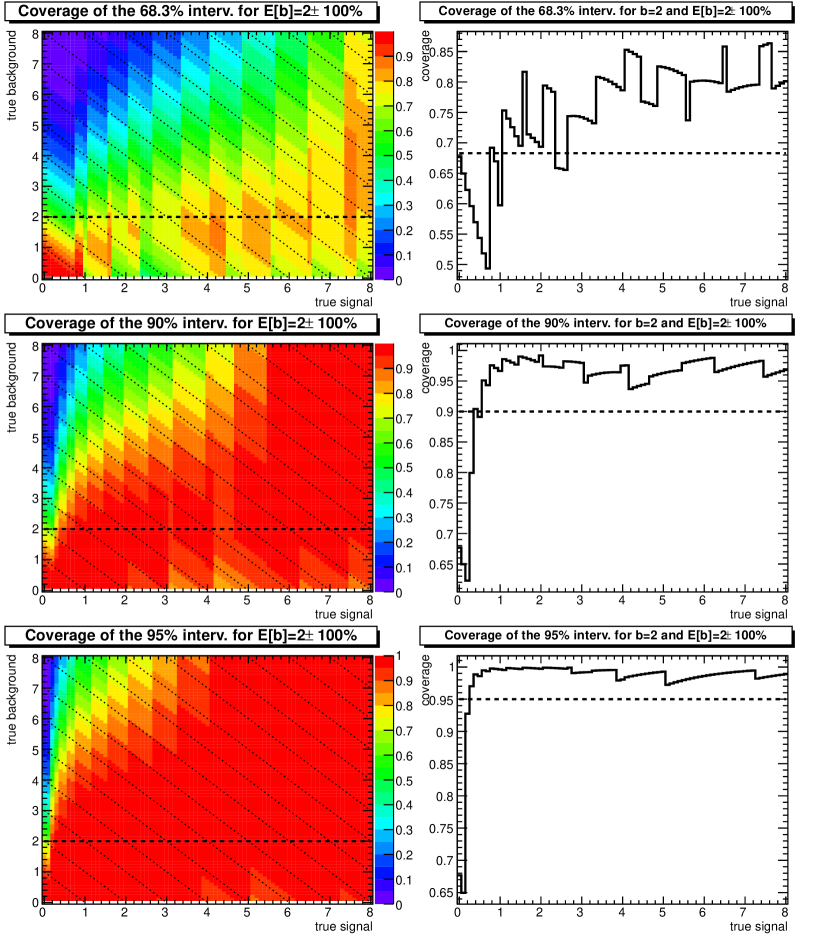
Figures 7, 8, 9 and 10 in appendix E show the coverage of 68.3%, 90% and 95% posterior credible intervals as a function of the true signal and background values. The diagonal structure is clearly due to the fact that we observe a single quantity, the number of counted events, which is the best estimator of the sum of true signal and background. This pattern is illustrated by the diagonal dotted lines, which characterize the loci with constant (and integer) sum of signal and background but different signal fraction. These figures also show the coverage as a function of the true signal alone, in the assumption that the true background coincides with the prior expectation (the 1D plot is the slice of the 2D plot at its left along the horizontal dashed line). As expected, a wider prior uncertainty gives more conservative results, in the sense that the overall tendency is to overcover, apart from very small values of the true signal, for which there is undercoverage. Instead, a narrow prior leads to a more symmetrical distribution of the actual coverage about the nominal one (the horizontal line in the right plots).

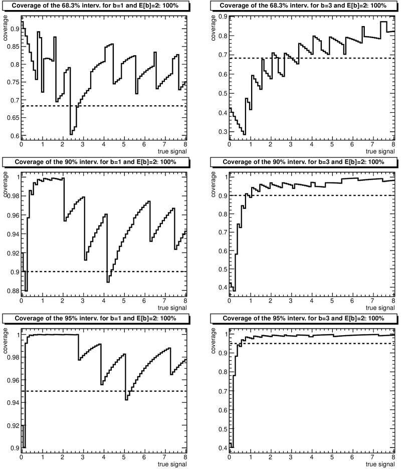
It is interesting to note what happens if the true signal is quite different from the prior expectation. In figure 11 (appendix E) the coverage of the solution which corresponds to a prior expectation of $E[b]=2$ with 100% uncertainty is shown when the true background is half of it (left plots) or 50% bigger (right plots). The tendency to overcover is more pronounced when the background is smaller than expected (which comes at no surprise). When the true background is half standard deviation higher than expected, the pattern is the same as for the case in which it matches the expectation (right plots of figure 10) but the fluctuations about the nominal coverage are less pronounced.

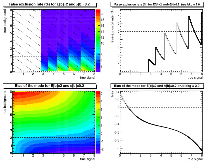
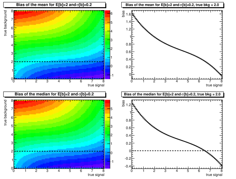
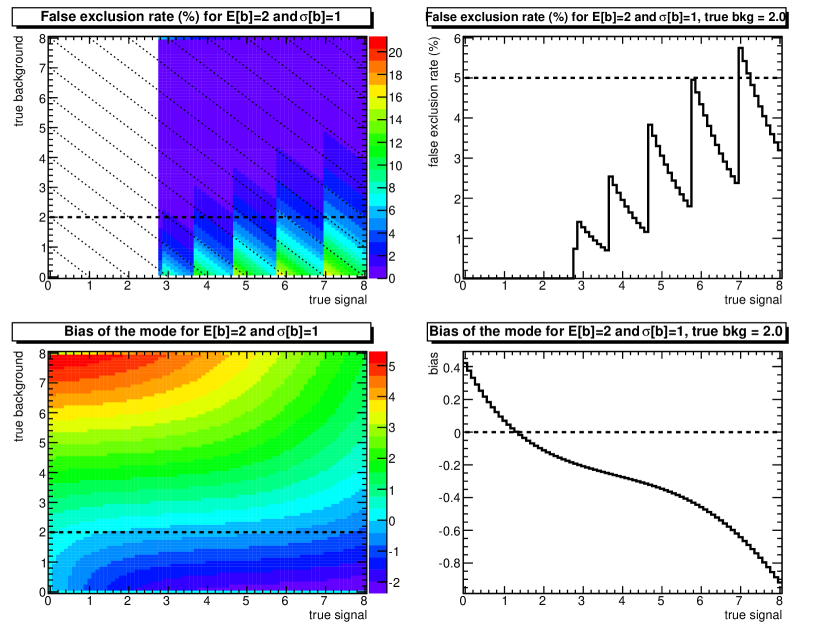
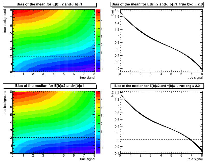
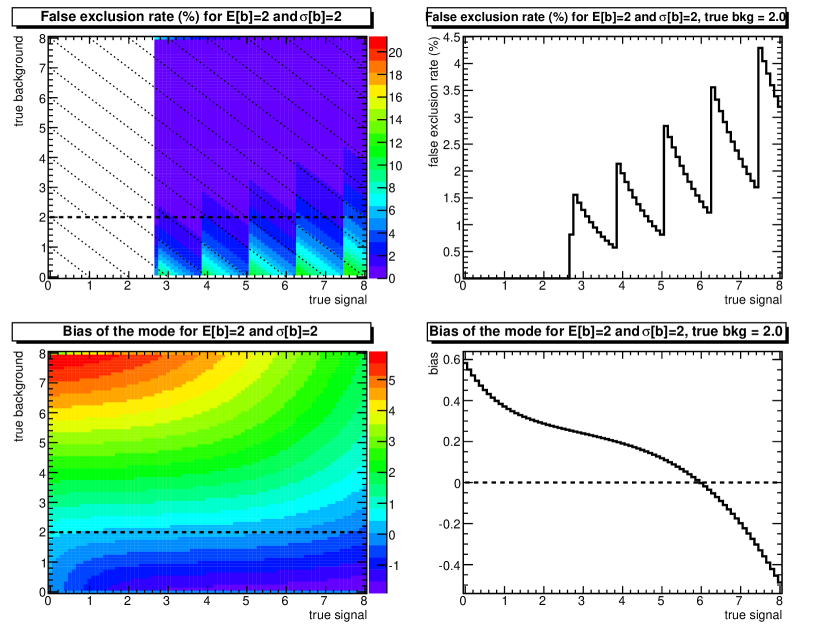
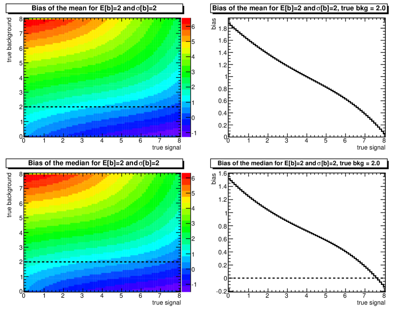
Other figures of merit for the solution are the false exclusion rate in case of 95% upper limits and the bias of the signal estimators. In appendix E the case of prior background expectation $E[b]=2$ counts with relative uncertainties of 10%, 50% and 100% are shown (figures 12, 13, 14, 15, 16). The diagonal pattern is still visible in the plots of the false exclusion rate as a function of the true signal and background, but not in the bias plots. The false exclusion rate may be larger than 5% when the prior uncertainty is small but this never happens when it is 100% or larger and it is very rare with 50% uncertainty. The bias of the different estimators, in all cases, is a monotonically decreasing function of the true signal. The mode tends to underestimate the true signal when the prior uncertainty is small, although bigger prior uncertainties tend to produce a more symmetric behaviour. The difference with respect to the true signal is usually less than one unit. On the other hand, both the mean and median tend to overestimate the true signal. Although the mean appears a bit more balanced than the mean, with a larger difference with respect to the true signal than the bias of the mode. In conclusion, the intuitive choice of the posterior peak as the best estimator for the true signal comes out to be the least biased estimator for small sample sizes.

6 Summary and conclusion

We considered the signal+background model in which both sources are independent Poisson processes, and there is available prior information about the background intensity $b$ encoded in a Gamma density of the form (2). Following the prescription by [12], the reference prior for the signal parameter $s$ is computed from the conditional model (9). The reference prior is proportional to the square root of the Fisher’s information (16), and is not normalizable. This is not a problem, because the reference posterior is a proper density, and the same also happens when using a $\delta$-function as the prior for the background. In this case the Jeffreys’ prior $\pi(s)\propto(s+b_{0})^{-1/2}$ is an improper density too, which cannot represent somebody’s degree of belief. The justification for the use of an improper prior is provided in the framework of the Bayesian reference analysis, in which the reference prior is defined as the mathematical device which maximizes the amount of missing information and does not represent an actual degree of belief [6].

Being an improper prior, one can always scale it by a constant: the normalization of the posterior density can be computed once the latter is known. For practical applications, we propose to adopt the improper prior (19) obtained by dividing the square root of the Fisher’s information by the value which it assumes for $s=0$. The resulting function assumes its maximum value (equal to one) at the origin and uniformly decreases for increasing values of $s$. Of course, one is also free to use equation (17) directly or to scale it by any other constant value.

The joint prior for our model is the improper function $\pi(s,b)=\pi(s)\,p(b)$ where $\pi(s)$ is defined by equation (19) (or any other function which is proportional to $|I(s)|^{1/2}$) and $p(b)$ is the Gamma density (2) which encodes the experimenter’s prior degree of belief about the background. Finally, the marginal reference posterior is proportional to the product of the reference prior (19) and the marginal likelihood (9):

$$p(s|k)\propto\left(\frac{\beta}{1+\beta}\right)^{\!\alpha}e^{-s}\,f(s;k,\alpha,\beta)\,\pi(s)\;.$$

A few examples of the application of this solution have been shown in section 5, together with their coverage, false exclusion rate, and the bias of different estimators of the true signal.

Appendix A Computing the conditional model

All results shown in this paper can be easily implemented once the function

$$f(s;k,\alpha,\beta)=\sum_{n=0}^{k}\binom{\alpha+n-1}{n}\frac{s^{k-n}}{(k-n)!\,(1+\beta)^{n}}$$

is available. Here we give some suggestion which lead to a fast evaluation of $f(s;k,\alpha,\beta)$.

Let us focus on each addendum first. It is better to work with the logarithms, because this avoids rounding problems related to expressions featuring very big and very small values:

$$\begin{split}&\binom{\alpha+n-1}{n}\frac{s^{k-n}}{(k-n)!\,(1+\beta)^{n}}=\\ &=\exp\left[\log\binom{\alpha+n-1}{n}+(k-n)\log s\right.\\ &\left.\quad-n\log(1+\beta)-\log(k-n)!\right]\end{split}$$

for $s>0$. For $s=0$ one computes directly the constant term which corresponds to $n=k$ in the sum from equation (18).

Plotting or integrating $f(s;k,\alpha,\beta)$ as a function of $s$, possibly for different values of $k$, implies that $\alpha,\beta$ are held constant during the computation. We now consider all terms from left to right.

The binomial coefficient is a function of $n$ with $\alpha$ fixed which increases faster than $\alpha^{n}$ and should be tabulated during the initialization phase. The following recursive relation holds:

$$\binom{\alpha+n-1}{n}=\begin{cases}1&\text{if}\;n=0\\ \alpha&\text{if}\;n=1\\ \displaystyle\frac{\alpha+n-1}{n}\,\binom{\alpha+n-2}{n-1}&\text{if}\;n\geq 2\\ \end{cases}$$

from which it follows that $a(n;\alpha)\equiv\log\binom{\alpha+n-1}{n}=\log[1+(\alpha-1)/n]+a(n-1;\alpha)$. For example, one can start by saving into a C++ vector the $a(n;\alpha)$ values for $n=0,\ldots,100$ and add more terms if needed later on, such that computing it during the loop over $n$ reduces to accessing the $n$-th element of the vector.

The value of $\log s$ should be computed once, outside the sum.

Because $\beta$ is fixed, $\log(1+\beta)$ is a constant term which should be only computed during the initialization phase, such that $b(n;\beta)\equiv n\log(1+\beta)=n\,b(1;\beta)$ is just a multiplication step. For intensive computations (like summations over $k=0,\ldots,\infty$ and/or integrations over $s\in[0,\infty[$) it can be useful to also store these values during the initialization phase.

Finally, the term $c(m)\equiv\log m!=\log m+c(m-1)$, where $m=k-n$, should be also computed during the initialization phase (say for $m=0,\ldots,100$) and stored into a vector for direct access inside the loop.

Appendix B Properties of $f(s;k,\alpha,\beta)$: Proofs

Proof of property 1

Property 3 is equivalent to the statement that $E[1]=1$, which is explicitly shown here:

$$\begin{split}E[1]&=\sum_{k=0}^{\infty}p(k|s)=\sum_{k=0}^{\infty}\left(\frac{\beta}{1+\beta}\right)^{\!\alpha}e^{-s}\,f(s;k,\alpha,\beta)\\ &=\left(\frac{\beta}{1+\beta}\right)^{\!\alpha}e^{-s}\,\sum_{k=0}^{\infty}\sum_{n=0}^{k}\frac{s^{k-n}}{(k-n)!}\binom{\alpha+n-1}{n}\frac{1}{(1+\beta)^{n}}\\ &=\left(\frac{\beta}{1+\beta}\right)^{\!\alpha}e^{-s}\,\sum_{n=0}^{\infty}\binom{\alpha+n-1}{n}\frac{1}{(1+\beta)^{n}}\sum_{k=n}^{\infty}\frac{s^{k-n}}{(k-n)!}\quad\;\left\{\sum_{k=0}^{\infty}\sum_{n=0}^{k}=\sum_{n=0}^{\infty}\sum_{n=k}^{\infty}\right\}\\ &=\left(\frac{\beta}{1+\beta}\right)^{\!\alpha}e^{-s}\,\sum_{n=0}^{\infty}\binom{\alpha+n-1}{n}\frac{1}{(1+\beta)^{n}}\sum_{m=0}^{\infty}\frac{s^{m}}{m!}\qquad\qquad\{m\equiv k-n\}\\ &=\left(\frac{\beta}{1+\beta}\right)^{\!\alpha}\sum_{n=0}^{\infty}\binom{\alpha+n-1}{n}\left(\frac{1}{1+\beta}\right)^{\!n}\\ &=\left(\frac{\beta}{1+\beta}\right)^{\!\alpha}\frac{1}{[1-1/(1+\beta)]^{\alpha}}=1\end{split}$$

where the following theorems have been used:

$$\sum_{m=0}^{\infty}\frac{s^{m}}{m!}=e^{s}\qquad\text{and}\qquad\sum_{n=0}^{\infty}\binom{\alpha+n-1}{n}x^{n}=\frac{1}{(1-x)^{\alpha}}\;.$$

Proof of property 2

We proceed by induction, showing that equation (11) holds for $n=1$ and that if it holds for $n-1$ then it must also hold for $n$. For $n=1$, by direct computation one obtains

$$\begin{split}f^{(1)}(s;k,\alpha,\beta)&=\sum_{n=0}^{k-1}\frac{s^{k-n-1}}{(k-n-1)!}\binom{\alpha+n-1}{n}\frac{1}{(1+\beta)^{n}}\\ &=\begin{cases}0&\text{if}\quad k=0\\ 1&\text{if}\quad k=1\\ f(s;k-1,\alpha,\beta)&\text{if}\quad k\geq 1\\ \end{cases}\end{split}$$

The next step is to show that if the property (11) holds for $n-1$ then it must also hold for $n$. For $n\leq k$ this is trivial (because $f^{(n-1)}$ is zero), while for $n>k$

$$\begin{split}\frac{\partial^{n}}{\partial s^{n}}f(s;k,\alpha,\beta)&=\frac{\partial}{\partial s}\frac{\partial^{n-1}}{\partial s^{n-1}}f(s;k,\alpha,\beta)\\ &=\frac{\partial}{\partial s}f(s;k-n+1,\alpha,\beta)\\ &=f(s;k-n,\alpha,\beta)\end{split}$$

where the last passage comes from $f^{(1)}(s;m,\alpha,\beta)=f(s;m-1,\alpha,\beta)$, in which $m=k-n+1$. This completes the proof.

Proof of property 3

Property 3 follows directly from the previous ones:

$$\begin{split}E\left[\frac{f^{(n)}(s;k,\alpha,\beta)}{f(s;k,\alpha,\beta)}\right]&=\sum_{k=0}^{\infty}\frac{f^{(n)}}{f}\,p(k|s)=\sum_{k=0}^{\infty}\frac{f^{(n)}}{f}\left(\frac{\beta}{1+\beta}\right)^{\!\alpha}e^{-s}\,f\\ &=\sum_{k=n}^{\infty}\left(\frac{\beta}{1+\beta}\right)^{\!\alpha}e^{-s}\,f^{(n)}(s;k,\alpha,\beta)\qquad\{k<n\Rightarrow f^{(n)}=0\}\\ &=\sum_{m=0}^{\infty}\left(\frac{\beta}{1+\beta}\right)^{\!\alpha}e^{-s}\,f(s;m,\alpha,\beta)\qquad\qquad\{m\equiv k-n\}\\ &=E[1]=1\end{split}$$ (21)

Appendix C Comparison with the DJP and PPSS papers

The notation used in the DJP and PPSS papers is different from the one adopted here:

DJP	PPSS	here	DJP	PPSS	here
$\sigma$	$s$	$s$	$b$	$b$	$\beta$
$\mu$	$\mu$	$b$	$y$	$Y$	$\alpha+\frac{1}{2}$
$\varepsilon$	1	1	$n$	$N$	$k$
— model—			— bkg prior —

The DJP model has one more parameter which is taken to be equal to 1 both here and in the PPSS paper. DJP wrote the Gamma density which represents such parameter in this form:

$$\pi(\varepsilon)=\frac{a(a\varepsilon)^{x-1/2}\,e^{-a\varepsilon}}{\Gamma(x+1/2)}$$

By formally setting $a=x$ and taking the limit $x\to\infty$ this distribution degenerates in the delta-function $\delta(\varepsilon-1)$, which is what is considered here and by PPSS.

The marginal model of DJP is

$$p(n|\sigma)=\left(\frac{a}{a+\sigma}\right)^{\!x+1/2}\left(\frac{b}{b+1}\right)^{\!y+1/2}S_{n}^{0}(\sigma)$$

where one polynomial appears of the following family

$$S_{n}^{m}(\sigma)=\sum_{k=0}^{n}\binom{k+x-\frac{1}{2}}{k}\binom{n-k+y-\frac{1}{2}}{n-k}\left(\frac{\sigma}{a+\sigma}\right)^{\!k}\frac{k^{m}}{(b+1)^{n-k}}$$

In the limit $a=x\to\infty$ the polynomials above become

$$S_{n}^{m}(\sigma)\to\sum_{k=0}^{n}\binom{n-k+y-\frac{1}{2}}{n-k}\frac{k^{m}\,\sigma^{k}}{k!\,(b+1)^{n-k}}$$

which in the notation of the PPSS paper coincides with $e^{s}\,T_{n}^{m}(s)$.

In the same limit, the DJP marginal model becomes

$$p(n|\sigma)\to e^{-\sigma}\left(\frac{b}{b+1}\right)^{\!y+1/2}\sum_{k=0}^{n}\binom{n-k+y-\frac{1}{2}}{n-k}\frac{\sigma^{k}}{k!\,(b+1)^{n-k}}$$

In the notation of this paper, the expression above becomes

$$\begin{split}p(n|\sigma)&=e^{-s}\left(\frac{\beta}{\beta+1}\right)^{\!\alpha}\sum_{k=0}^{n}\binom{n-k+\alpha-1}{n-k}\frac{s^{k}}{k!\,(\beta+1)^{n-k}}=\\ \left\{\text{set $m\equiv n-k$ in the sum}\right\}\\ &=e^{-s}\left(\frac{\beta}{\beta+1}\right)^{\!\alpha}\sum_{m=0}^{n}\binom{m+\alpha-1}{m}\frac{s^{n-m}}{(n-m)!\,(\beta+1)^{m}}=\\ &=e^{-s}\left(\frac{\beta}{\beta+1}\right)^{\!\alpha}f(s;n,\alpha,\beta)\quad\leftarrow\text{eq.~{}(\ref{eq-marg-mod-2}) of section~{}\ref{sec-marginal-model}.}\end{split}$$

In a similar way, one can write the marginal model in the PPSS paper in the form of our equation (9), because the function $e^{-s}\,f(s;n,\alpha,\beta)$ is the same thing as the PPSS function $T_{n}^{0}(s)$.

Appendix D Model with a degenerate background prior

If we have a certain knowledge about the background yield, the prior for $b$ becomes a delta-function $p(b)=\delta(b-b_{0})$, which is the degenerate form of a Gamma density with parameters $\beta=\alpha/b_{0},\alpha\to\infty$. In this case, the marginal model is

$$p(k|s)=\int_{0}^{\infty}\text{Poi}(k|s+b)\,\delta(b-b_{0})\,\text{d}b=\text{Poi}(k|s+b_{0})$$

whose logarithm is

$$\log p(k|s)=k\log(s+b_{0})-s-b_{0}-\log k!\;.$$

The second derivative of the logarithm of the marginal model is $-k/(s+b_{0})^{2}$ such that the Fisher’s information is

$$\begin{split}I(s)&=-E\left[\left(\frac{\partial^{2}}{\partial s^{2}}\log p(k|s)\right)\right]\\ &=e^{-s-b_{0}}\,\sum_{k=0}^{\infty}\frac{k}{(s+b_{0})^{2}}\frac{(s+b_{0})^{k}}{k!}\end{split}$$

whose 0-th element is null, hence we can write a sum starting from $k=1$ and then introduce a new index $n=k-1$:

$$\begin{split}I(s)&=e^{-s-b_{0}}\,\sum_{k=1}^{\infty}\frac{(s+b_{0})^{k-2}}{(k-1)!}\\ &=\frac{e^{-s-b_{0}}}{s+b_{0}}\,\sum_{n=0}^{\infty}\frac{(s+b_{0})^{n}}{n!}=\frac{1}{s+b_{0}}\end{split}$$

from which one finds the reference prior as $\pi(s)\propto|I(s)|^{1/2}=(s+b_{0})^{-1/2}$.

We now verify that one gets the same solution when defining $\beta=\alpha/b_{0}$ and considering the limit $\alpha\to\infty$ in our model. First, let’s consider the function $f(s;k,\alpha,\beta)$:

$$\begin{split}f(s;k,\alpha,\alpha/b_{0})&=\sum_{n=0}^{k}\frac{\Gamma(\alpha+n)}{\Gamma(\alpha)}\frac{s^{k-n}}{(k-n)!}\frac{b_{0}^{n}}{n!\,(b_{0}+\alpha)^{n}}\\ &\xrightarrow{\alpha\to\infty}\sum_{n=0}^{k}\frac{s^{k-n}\,b_{0}^{n}}{(k-n)!\,n!}=\frac{(s+b_{0})^{k}}{k!}\;.\end{split}$$

Let’s call this limit $f(s;k)=(s+b_{0})^{k}/k!$. Next, consider

$$\begin{split}\left(\frac{\beta}{1+\beta}\right)^{\!\alpha}&=\left(\frac{\alpha}{\alpha+b_{0}}\right)^{\!\alpha}\\ &=\left(1+\frac{b_{0}}{\alpha}\right)^{\!-\alpha}\xrightarrow{\alpha\to\infty}e^{-b_{0}}\;.\end{split}$$

Finally, in this limit the Fisher’s information (17) becomes

$$\begin{split}I(s)&=e^{-s-b_{0}}\,\sum_{n=0}^{\infty}\frac{f^{2}(s;n)}{f(s;n+1)}-1\\ &=e^{-s-b_{0}}\,\sum_{n=0}^{\infty}\left[\frac{(s+b_{0})^{n}}{n!}\right]^{2}\frac{(n+1)!}{(s+b_{0})^{n+1}}-1\end{split}$$

The 0-th term in the sum is $(s+b_{0})^{-1}$ and, from the 1-st term on, the factorial $(n-1)!$ is well defined, such that we can write

$$I(s)=\frac{e^{-s-b_{0}}}{s+b_{0}}+e^{-s-b_{0}}\,\left[\sum_{n=1}^{\infty}\frac{(s+b_{0})^{n-1}}{(n-1)!}\frac{n+1}{n}\right]-1$$

The sum above can be rewritten

$$\begin{split}\sum_{n=1}^{\infty}&\frac{(s+b_{0})^{n-1}}{(n-1)!}\frac{n+1}{n}=\sum_{m=0}^{\infty}\frac{(s+b_{0})^{m}}{m!}\left(1+\frac{1}{m+1}\right)\\ &=e^{s+b_{0}}+\sum_{m=0}^{\infty}\frac{(s+b_{0})^{m}}{m!\,(m+1)}\\ &=e^{s+b_{0}}+(s+b_{0})^{-1}\sum_{m=0}^{\infty}\frac{(s+b_{0})^{m+1}}{(m+1)!}\\ &=e^{s+b_{0}}+(s+b_{0})^{-1}\sum_{n=1}^{\infty}\frac{(s+b_{0})^{n}}{n!}\\ &=e^{s+b_{0}}+\frac{e^{s+b_{0}}-1}{s+b_{0}}\end{split}$$

which inserted in $I(s)$ gives

$$\begin{split}I(s)&=\frac{e^{-s-b_{0}}}{s+b_{0}}+e^{-s-b_{0}}\,\left[e^{s+b_{0}}+\frac{e^{s+b_{0}}-1}{s+b_{0}}\right]-1\\ &=\frac{1}{s+b_{0}}\;,\end{split}$$

exactly the same expression which one obtains when starting directly with the delta-function.

Appendix E Summaries of the solutions and their properties

The following tables and plots provide a summary of the marginal posteriors for the signal in the cases of $E[b]=2$ prior background expectation with relative uncertainty of 10%, 20%, 50% and 100%, and of their coverage. In addition, the false exclusion rate and biases of the posterior mode, mean and median are shown.

Tables 3, 4, 5 and 6 report the left and right bounds of the 68.3%, 90%, 95% credible intervals, plus mean, median, mode, variance, skewness and excess kurtosis. The coverage of such intervals has been studied for different observations ($k=0,1,\ldots,15$ counts) and the average over $k$ is shown in figures 7, 8, 9 and 10. Because of the limited range in $k$ considered here, the coverage is to be intended as a first approximation when the sum of true signal and background exceeds 10–12 counts. In the 2D plots, the diagonal lines have constant sum of true signal and background, whereas the horizontal line identifies the slice which is shown in the corresponding 1D plot. The horizontal line in 1D plots shows the nominal coverage.

Figures 12, 13, 14, 15, 16, and 17 show the false exclusion rate (which is the average fraction of times the true signal is above the 95% upper limit) and the bias of the posterior mode, mean and median (which is the difference between the estimator and the true signal), as a function of true signal and background (left plots) and as a function of the true signal alone, for the case in which the true background coincides with the prior expectation. Only the posteriors obtained with a prior background expectation $E[b]=2$ counts with relative uncertainties of 10%, 50% and 100% are shown. The empty region in the 2D plots of the false exclusion rate corresponds to identically zero exclusion rate: in this region the true signal is always smaller than the upper limit.

nObs	L95	L90	L68	Mean	Median	Mode	R68	R90	R95	Vari.	Skew.	Kurt.
0	0.00	0.00	0.00	0.88	0.60	0.00	1.01	2.08	2.77	0.80	2.11	6.76
1	0.00	0.00	0.00	1.16	0.83	0.00	1.36	2.68	3.48	1.26	1.88	5.19
2	0.00	0.00	0.00	1.56	1.18	0.00	1.86	3.46	4.38	1.94	1.62	3.73
3	0.09	0.17	0.00	2.10	1.71	0.52	2.55	5.44	6.44	2.87	1.36	2.57
4	0.16	0.31	0.87	2.80	2.41	1.51	4.73	6.64	7.70	4.00	1.14	1.75
5	0.34	0.59	1.39	3.63	3.26	2.51	5.85	7.91	9.04	5.21	0.96	1.24
6	0.67	1.05	2.07	4.55	4.20	3.51	7.01	9.21	10.40	6.38	0.83	0.96
7	1.17	1.65	2.83	5.51	5.18	4.51	8.19	10.51	11.76	7.48	0.74	0.80
8	1.77	2.32	3.64	6.50	6.17	5.51	9.36	11.80	13.10	8.52	0.69	0.70
9	2.43	3.04	4.46	7.50	7.17	6.50	10.53	13.08	14.43	9.54	0.65	0.63
10	3.12	3.78	5.30	8.50	8.17	7.50	11.69	14.34	15.74	10.54	0.61	0.57
11	3.82	4.53	6.15	9.50	9.16	8.50	12.84	15.59	17.04	11.54	0.59	0.52
12	4.54	5.29	7.00	10.50	10.16	9.50	13.99	16.83	18.33	12.54	0.56	0.48
13	5.27	6.06	7.86	11.50	11.16	10.50	15.13	18.06	19.60	13.54	0.54	0.44
14	6.00	6.84	8.73	12.50	12.16	11.50	16.27	19.28	20.87	14.54	0.52	0.41
15	6.75	7.62	9.60	13.50	13.16	12.50	17.40	20.50	22.12	15.54	0.51	0.39

Table 3: Posterior summary for $E[b]=2\pm 0.2$ as a function of the number of observed events.

nObs	L95	L90	L68	Mean	Median	Mode	R68	R90	R95	Vari.	Skew.	Kurt.
0	0.00	0.00	0.00	0.88	0.60	0.00	1.01	2.08	2.78	0.81	2.10	6.73
1	0.00	0.00	0.00	1.17	0.84	0.00	1.38	2.71	3.51	1.28	1.86	5.09
2	0.00	0.00	0.00	1.59	1.21	0.00	1.90	3.50	4.42	1.98	1.60	3.64
3	0.09	0.17	0.53	2.13	1.74	0.57	3.75	5.50	6.49	2.92	1.35	2.50
4	0.17	0.32	0.88	2.83	2.44	1.55	4.77	6.69	7.76	4.06	1.13	1.71
5	0.33	0.59	1.39	3.65	3.28	2.54	5.88	7.95	9.09	5.28	0.95	1.21
6	0.64	1.02	2.06	4.56	4.21	3.53	7.04	9.25	10.44	6.47	0.82	0.93
7	1.12	1.61	2.81	5.52	5.18	4.53	8.21	10.54	11.79	7.59	0.73	0.77
8	1.71	2.28	3.61	6.50	6.17	5.52	9.39	11.83	13.14	8.65	0.67	0.68
9	2.37	2.99	4.44	7.50	7.17	6.52	10.55	13.10	14.46	9.67	0.63	0.61
10	3.06	3.73	5.28	8.50	8.17	7.52	11.71	14.37	15.77	10.68	0.60	0.55
11	3.77	4.49	6.13	9.50	9.17	8.52	12.86	15.62	17.07	11.68	0.58	0.51
12	4.49	5.25	6.98	10.50	10.17	9.51	14.01	16.85	18.36	12.68	0.55	0.47
13	5.22	6.02	7.84	11.50	11.17	10.51	15.15	18.08	19.63	13.68	0.53	0.43
14	5.96	6.80	8.71	12.50	12.17	11.51	16.28	19.30	20.89	14.67	0.52	0.40
15	6.71	7.59	9.58	13.50	13.17	12.51	17.41	20.52	22.14	15.67	0.50	0.38

Table 4: Posterior summary for $E[b]=2\pm 0.4$ as a function of the number of observed events.

nObs	L95	L90	L68	Mean	Median	Mode	R68	R90	R95	Vari.	Skew.	Kurt.
0	0.00	0.00	0.00	0.89	0.61	0.00	1.02	2.10	2.80	0.82	2.10	6.68
1	0.00	0.00	0.00	1.26	0.92	0.00	1.48	2.86	3.67	1.39	1.78	4.64
2	0.00	0.00	0.00	1.73	1.35	0.00	2.08	3.74	4.68	2.18	1.51	3.20
3	0.10	0.20	0.61	2.31	1.92	0.82	4.02	5.79	6.80	3.19	1.27	2.18
4	0.17	0.33	0.95	3.00	2.62	1.77	5.03	6.98	8.06	4.38	1.06	1.49
5	0.30	0.56	1.42	3.78	3.43	2.73	6.11	8.22	9.37	5.67	0.90	1.05
6	0.52	0.91	2.02	4.65	4.32	3.70	7.24	9.48	10.69	6.97	0.77	0.78
7	0.87	1.39	2.72	5.57	5.26	4.68	8.38	10.75	12.02	8.22	0.67	0.63
8	1.36	2.00	3.49	6.52	6.22	5.66	9.53	12.02	13.34	9.41	0.60	0.54
9	1.96	2.68	4.31	7.50	7.21	6.64	10.69	13.28	14.66	10.52	0.55	0.49
10	2.63	3.42	5.14	8.49	8.20	7.63	11.84	14.53	15.96	11.59	0.52	0.46
11	3.34	4.18	5.99	9.49	9.20	8.62	12.98	15.78	17.25	12.62	0.49	0.43
12	4.08	4.96	6.85	10.49	10.19	9.61	14.12	17.01	18.52	13.63	0.48	0.41
13	4.83	5.74	7.72	11.49	11.19	10.60	15.26	18.23	19.79	14.63	0.46	0.38
14	5.60	6.54	8.59	12.49	12.19	11.60	16.39	19.45	21.05	15.62	0.45	0.36
15	6.36	7.34	9.47	13.49	13.19	12.59	17.52	20.66	22.30	16.62	0.44	0.34

Table 5: Posterior summary for $E[b]=2\pm 1$ as a function of the number of observed events.

nObs	L95	L90	L68	Mean	Median	Mode	R68	R90	R95	Vari.	Skew.	Kurt.
0	0.00	0.00	0.00	0.84	0.56	0.00	0.96	2.03	2.74	0.79	2.17	7.17
1	0.00	0.00	0.00	1.36	1.03	0.00	1.62	3.04	3.86	1.52	1.69	4.18
2	0.00	0.00	0.00	1.95	1.59	0.00	2.37	4.10	5.05	2.48	1.37	2.63
3	0.12	0.24	0.74	2.60	2.24	1.40	4.45	6.26	7.28	3.64	1.13	1.72
4	0.18	0.36	1.08	3.31	2.97	2.32	5.50	7.49	8.59	4.96	0.94	1.14
5	0.27	0.53	1.51	4.08	3.77	3.26	6.58	8.73	9.90	6.41	0.78	0.76
6	0.39	0.76	2.03	4.90	4.62	4.20	7.68	9.98	11.21	7.92	0.65	0.52
7	0.56	1.07	2.64	5.76	5.52	5.16	8.79	11.22	12.51	9.46	0.55	0.37
8	0.79	1.46	3.32	6.65	6.44	6.12	9.92	12.46	13.81	10.99	0.46	0.29
9	1.11	1.95	4.05	7.58	7.39	7.08	11.04	13.70	15.10	12.47	0.38	0.25
10	1.52	2.54	4.84	8.52	8.35	8.05	12.17	14.94	16.39	13.89	0.33	0.23
11	2.02	3.20	5.66	9.49	9.33	9.02	13.30	16.16	17.66	15.24	0.28	0.24
12	2.62	3.92	6.50	10.46	10.31	10.00	14.43	17.39	18.93	16.53	0.24	0.26
13	3.29	4.69	7.36	11.45	11.30	10.98	15.56	18.60	20.19	17.75	0.22	0.28
14	4.03	5.49	8.23	12.44	12.29	11.96	16.68	19.81	21.44	18.92	0.20	0.30
15	4.81	6.31	9.11	13.44	13.28	12.94	17.80	21.01	22.68	20.04	0.19	0.32

Table 6: Posterior summary for $E[b]=2\pm 2$ as a function of the number of observed events.

Figure 7: Coverage of the 95% (top), 90% (middle), 68.3% (bottom) posterior credible intervals for $E[b]=2\pm 0.2$ as a function of the true signal and background (left panel) and as a function of the true signal alone in case the true background coincides with the prior expectation (left panel).

Figure 8: Coverage of the 95% (top), 90% (middle), 68.3% (bottom) posterior credible intervals for $E[b]=2\pm 0.4$ as a function of the true signal and background (left panel) and as a function of the true signal alone in case the true background coincides with the prior expectation (left panel).

Figure 9: Coverage of the 95% (top), 90% (middle), 68.3% (bottom) posterior credible intervals for $E[b]=2\pm 1$ as a function of the true signal and background (left panel) and as a function of the true signal alone in case the true background coincides with the prior expectation (left panel).

Figure 10: Coverage of the 95% (top), 90% (middle), 68.3% (bottom) posterior credible intervals for $E[b]=2\pm 2$ as a function of the true signal and background (left panel) and as a function of the true signal alone in case the true background coincides with the prior expectation (left panel).

Figure 11: Coverage of the 95% (top), 90% (middle), 68.3% (bottom) posterior credible intervals for $E[b]=2\pm 2$ as a function of the true signal, when the true background is half of the background expectation (left) or 50% bigger (right).

q

Figure 12: Top: false exclusion rate as a function of the true signal and background (top-left) and of the true signal alone for the case in which the true background coincides with the prior expectation (top-right). Bottom: bias of the posterior mode as a function of the true signal and background (bottom-left) and of the true signal alone for the case in which the true background coincides with the prior expectation (bottom-right). The posterior corresponds to a prior background expectation of 2 counts with 10% relative uncertainty.

Figure 13: Bias of the posterior mean (top) and median (bottom) as a function of the true signal and background (left plots) and of the true signal alone for the case in which the true background coincides with the prior expectation (right plots). The posterior corresponds to a prior background expectation of 2 counts with 10% relative uncertainty.

Figure 14: Top: false exclusion rate as a function of the true signal and background (top-left) and of the true signal alone for the case in which the true background coincides with the prior expectation (top-right). Bottom: bias of the posterior mode as a function of the true signal and background (bottom-left) and of the true signal alone for the case in which the true background coincides with the prior expectation (bottom-right). The posterior corresponds to a prior background expectation of 2 counts with 50% relative uncertainty.

Figure 15: Bias of the posterior mean (top) and median (bottom) as a function of the true signal and background (left plots) and of the true signal alone for the case in which the true background coincides with the prior expectation (right plots). The posterior corresponds to a prior background expectation of 2 counts with 50% relative uncertainty.

Figure 16: Top: false exclusion rate as a function of the true signal and background (top-left) and of the true signal alone for the case in which the true background coincides with the prior expectation (top-right). Bottom: bias of the posterior mode as a function of the true signal and background (bottom-left) and of the true signal alone for the case in which the true background coincides with the prior expectation (bottom-right). The posterior corresponds to a prior background expectation of 2 counts with 100% relative uncertainty.

Figure 17: Bias of the posterior mean (top) and median (bottom) as a function of the true signal and background (left plots) and of the true signal alone for the case in which the true background coincides with the prior expectation (right plots). The posterior corresponds to a prior background expectation of 2 counts with 100% relative uncertainty.

References

- [1] D. Casadei, Statistical methods used in ATLAS for exclusion and discovery, proceed. of PHYSTAT2011, CERN, 17-20 Jan 2011, \hrefhttp://arXiv.org/abs/1108.2288arXiv: 1108.2288.
- [2] S.I. Bityukov and N.V. Krasnikov, NIM A452 (2000) 518, 10.1016/S0168-9002(00)00454-X; S.I. Bityukov, N.V. Krasnikov, V. Smirnova, AIP Conf. Proc. 1305 (2010) 235, 10.1063/1.3573622.
- [3] G. Cowan, K. Cranmer, E. Gross, O. Vitells, Asymptotic formulae for likelihood-based tests of new physics, Eur. Phys. J. C71 (2011) 1554, 10.1140/epjc/s10052-011-1554-0.
- [4] L. Demortier, S. Jain, H.B. Prosper, Reference priors for high energy physics, Phys. Rev. D 82 (2010) 034002. Phys. Rev. D822010034002.
- [5] M. Pierini, H.B. Prosper, S. Sekmen, M. Spiropulu, Priors for New Physics, 2011, \hrefhttp://arXiv.org/abs/1108.0523arXiv: 1108.0523
- [6] J.M. Bernardo, Reference analysis, in Handbook of Statistics 25 (D.K. Dey, C.R. Rao ed.), Elsevier (2005), pp. 17, 10.1016/S0169-7161(05)25002-2.
- [7] J.O. Berger, J.M. Bernardo, D. Sun, The formal definition of reference priors, The Annals of Statistics 37 (2009) 905, 10.1214/07-AOS587.
- [8] J.O. Berger, The Bayesian Approach to Discovery, Proc. of PHYSTAT 2011, 17–20 Jan 2011, CERN, Geneva, Switzerland, \hrefhttp://cdsweb.cern.ch/record/1306523CERN-2011-006, ISBN 978-92-9083-367-3.
- [9] L. Demortier, Open issues in the wake of Banff 2010, Proc. of PHYSTAT 2011, 17–20 Jan 2011, CERN, Geneva, Switzerland, \hrefhttp://cdsweb.cern.ch/record/1306523CERN-2011-006, ISBN 978-92-9083-367-3.
- [10] J.M. Bernardo, Bayes and Discovery: Objective Bayesian Hypothesis Testing, Proc. of PHYSTAT 2011, 17–20 Jan 2011, CERN, Geneva, Switzerland, \hrefhttp://cdsweb.cern.ch/record/1306523CERN-2011-006, ISBN 978-92-9083-367-3.
- [11] J.M. Bernardo, “Bayesian Statistics”, in Encyclopedia of Life Support Systems (EOLSS). Probability and Statistics (ed. by R. Viertl), Oxford, 2003, UNESCO (www.eolss.net).
- [12] D. Sun and J.O. Berger, Reference priors with partial information, Biometrika 85 (1998) 55, 10.1093/biomet/85.1.55.
- [13] J.M. Bernardo and A.F.M. Smith, Bayesian theory, Wiley, 1994, 10.1002/9780470316870.
- [14] J.M. Bernardo, Modern Bayesian inference: Foundations and objective methods, in Philosophy of Statistics (P. Bandyopadhyay, M. Forster ed.), Elsevier, 2009, \hrefhttp://www.elsevierdirect.com/ISBN/9780444518620/Philosophy-of-StatisticsISBN:978-0-444-51862-0.
- [15] K. Nakamura et al. (Particle Data Group), 2010 Review of Particle Physics, J. Phys. G 37, 075021 (2010), 10.1088/0954-3899/37/7A/075021.
- [16] J.M. Bernardo, Ojective Bayesian point and region estimation in location-scale models, \hrefhttp://vivianita.cadiretes.cesca.cat/index.php/SORT/article/view/73887Sort 31 (2007) 3-44.
- [17] R.D. Cousins, K.E. Hymes, J. Tucker, Frequentist Evaluation of Intervals Estimated for a Binomial Parameter and for the Ratio of Poisson Means, NIM A 612 (2010) 388–398, 10.1016/j.nima.2009.10.156, \hrefhttp://arXiv.org/abs/0905.3831arXiv: 0905.3831