Origin of spontaneous broken mirror symmetry of vortex lattices in Nb

Abstract

Combining the microscopic Eilenberger theory with the first principles band calculation, we investigate the stable flux line lattice (FLL) for a field applied to the four-fold axis; $H\parallel[001]$ in cubic Nb. The observed FLL transformation along $H_{c2}$ is almost perfectly explained without adjustable parameter, including the tilted square, scalene triangle with broken mirror symmetry, and isosceles triangle lattices upon increasing $T$. We construct a minimum Fermi surface model to understand those morphologies, in particular the stability of the scalene triangle lattice attributed to the lack of the mirror symmetry about the Fermi velocity maximum direction in k-space.

A series of elemental metal superconductors, Nb, V, Al, $\cdots$ have a long history since its discovery of Hg in 1911. Those are now regarded as a “conventional” superconductor where in fact the energy gap is isotropic and electron-phonon mechanism is known to work well. Thus it seems that no mystery remains there and every superconducting aspect is well understood and controlled since Nb is known to be wide practical applications from Nb-SQUID magnetometers to superconducting cavities for particle acceleratorsnature . However, recent small angle neutron scattering (SANS) experiments on Nb discover plethora of the mysterious vortex morphologylaver1 ; laver2 ; muhlbauer , requiring us a consistent understanding of flux line lattice symmetry changes upon varying the applied field direction continuously, that should satisfy a global constraint imposed by the hairy ball theoremhairy , namely any local change of FLL symmetry must be consistent with the change viewed globally.

Among them recent finding by Laver et al. laver1 is particularly intriguing: They find a novel FLL whose half unit cell is a scalene triangle by SANS experiment on Nb under a field applied along $H\parallel[001]$ direction. By varying $H$ and $T$ they have succeeded in constructing the vortex lattice phase diagram (see Fig.1(b)). Along the $H_{c2}$ line from low $T$ and high $H$ the square lattice tilted by $10.9^{\circ}$ from the [100] direction changes into a scalene lattice followed by an isosceles lattice that is stabilized at higher $T$. Although the tilted square lattice has been known for a quite long time experimentally without any theoretical understandingweber , the discovery of the scalene lattice is new and intriguing since the scalene lattice breaks the fundamental mirror symmetry spontaneously in cubic crystalline Nb. Notice that among various superconductors, conventional and unconventional, there is no known case to exhibit either scalene triangle or tilted square FLL under the four-fold symmetric field configuration, namely, tetragonal crystals under $H\parallel[001]$ such as CeCoIn₅ bianch , Sr₂RuO₄ riseman , La_1.83Sr_0.17O₄ gilardi , ErNi₂B₂C morten1 , YNi₂B₂C morten2 , and TmNi₂B₂C debeer .

According to Takanaka takanaka who is a pioneer in this field of theoretical FFL morphology studies, the free energy of FLL contains the so-called phasing energy that depends on the relative orientation between the FLL and underlying crystal lattice. This implies that the observed tilted square lattice may be stabilized by this phasing energy. This is expanded in terms of the higher order harmonics of the four-fold symmetry ($\theta$ is the angle from the [100] direction), $F_{phasing}=\Sigma_{n=1,2,\cdots}A_{4n}\cos 4n\theta$ whose minima may give rise to the tilting angle $\theta=10.9^{\circ}$ from the [100] direction, meaning that at least two or more higher harmonics are simultaneously non-vanishing.

Here the purposes of this paper are two-fold: The first principles band calculation based on density functional theory (DFT) yields precise information on the electronic properties of the normal state in general. By combining it with the microscopic Eilenberger theory, we can establish a truly first principles framework for a superconductor, in particularly for vortex state under an applied field without any adjustable parameters. In order to benchmark it we apply this to explain those intriguing vortex morphologies, which will turn out that this framework is remarkably successful.

Thus the second purpose is to understand the physical origin for the scalene FLL structure by constructing a minimum model Hamiltonian to describe the FLL transformation mentioned above. The mirror symmetry breaking with the scalene FLL is attributed to the special character of the Nb electronic band structure. This study points to the fact that our combined framework of DFT and the Eilenberger theory paves the way to truly first principles theory for superconductors properties under a field without adjustable parameter. Previously several attempts have been done to perform this program, but those are limited to either discussions on $H_{c2}$kita or resorting to approximate solutions for Eilenberger equationnagai .

In order that our calculations are tractable within a reasonable computational time frame, we limit our discussion along $H_{c2}$, that reduces significantly the computational time because we must minimize the free energy in the multi-dimensional parameter space spanned by the FLL unit cell shape and its orientation relative to the underlying crystal axes.

The quasiclassical Eilenberger theoryeilenberger ; ichioka ; nakai is quantitatively valid when $\xi\gg 1/k_{\rm F}$ ($k_{\rm F}$ is the Fermi wave number and $\xi$ is the superconducting coherence length). The quasiclassical Green’s functions $g(\omega_{n},{\bf k},{\bf r})$, $f(\omega_{n},{\bf k},{\bf r})$, and $f^{\dagger}(\omega_{n},{\bf k},{\bf r})$ are calculated by the Eilenberger equation

$$\left\{\omega_{n}+{\bf v}_{F}\cdot\left(\nabla+{\rm i}{\bf A}\right)\right\}f(\omega_{n},{\bf k},{\bf r})=\Delta g(\omega_{n},{\bf k},{\bf r}),$$

$$\left\{\omega_{n}-{\bf v}_{F}\cdot\left(\nabla-{\rm i}{\bf A}\right)\right\}f^{\dagger}(\omega_{n},{\bf k},{\bf r})=\Delta^{\ast}g(\omega_{n},{\bf k},{\bf r}),\quad$$ (1)

where $g=(1-ff^{\dagger})^{1/2}$, ${\rm Re}$$g>0$, $\bf A$ is the vector potential and ${\bf v}_{F}$ is the Fermi velocity. At $t=T/T_{c}$, the self-consistent gap equation is given by

$$\Delta\ln t=t\sum_{\omega_{n}}\left(\langle f(\omega_{n},{\bf k},{\bf r})\rangle_{\bf k}-{\Delta\over|\omega_{n}|}\right),$$ (2)

where $\langle\cdots\rangle_{\bf k}=\int d\theta D(\theta,\epsilon_{F})(\cdots)$ with $D(\theta,\epsilon_{F})$ being the angle-resolved density of states (AR-DOS) at the Fermi surface.

Along $H_{c2}$, we linearize the Eilenberger equation as

$$[\omega_{n}+{\bf v}_{F}\cdot(\nabla+{\rm i}{\bf A})]f(\omega_{n},{\bf k},{\bf r})=\Delta.$$ (3)

By expanding $\Delta$ and $f(\omega_{n},{\bf k},{\bf r})$ in terms of the Landau-Bloch function $\psi_{N,{\bf q}}({\bf r})$ whose $N$-th coefficients are $\Delta_{N}$ and $f_{N}(\omega_{n},{\bf k})$, we can obtain the eigenvalue equation for $\Delta$, from which $H_{c2}$, $\Delta_{N}$ and $f_{N}(\omega_{n},{\bf k})$ are evaluatedkita2 . Those eigenfunctions lead to the gap function $\Delta({\bf r})$ and the quasiclassical Green’s function $f(\omega_{n},{\bf k},{\bf r})$.

In order to compare various FLL forms to find the most stable vortex configuration near $H_{c2}$, we have to calculate the free energy $F$ given by

$$F=\tilde{\kappa}^{2}\overline{(\nabla\times{\bf A})^{2}}+\overline{|\Delta|^{2}}\ln t+2t\sum_{\omega_{n}>0}\left[{\overline{|\Delta|^{2}}\over\omega_{n}}-\overline{\langle I\rangle}\right]$$ (4)

with $I=(g-1)[2\omega_{n}+{\bf v}_{F}\cdot(\nabla\ln(f/f^{\dagger})+2i{\bf A})]+(f\Delta^{\ast}+\Delta f^{\dagger})$. Via the Abrikosov identity and expanding the normalization condition up to the next order; $g\sim 1-ff^{\dagger}/2-(ff^{\dagger})^{2}/8$, we obtain the free energy valid near $H_{c2}$ as nakai

$${F\over\tilde{\kappa}^{2}}=B^{2}-{(B-H_{c2})^{2}\over{\tilde{F}+1}},$$ (5)

$$\tilde{F}={t\over{4\tilde{\kappa}^{2}\bar{h}_{s}^{2}}}\sum_{\omega_{n}>0}\overline{\langle{ff^{\dagger}(f\Delta^{\ast}+\Delta f^{\dagger})}\rangle_{\bf k}}-{\overline{h_{s}^{2}}\over\bar{h}_{s}^{2}},$$ (6)

where $\overline{(\cdots)}$ denotes the spatial average within a unit cell, and $\bar{h}_{s}$ is the magnetic field induced by supercurrent. $B=H+\bar{h}_{s}$ and $\tilde{\kappa}^{2}=7\zeta(3)\kappa^{2}/18$. Since we know that the vortex morphology is independent of GL parameter $\kappa$suzuki , here we have used a large $\kappa$. The free energy minimum corresponds to the minimum of $\tilde{F}$ that gives the stable vortex lattice configuration.

The Fermi velocity ${\bf v}_{F}(\theta)$ and AR-DOS $D(\theta,\epsilon_{F})$ are evaluated by using tetrahedron method within DFTwien2k . The first Brillouin zone is divided into 135³ parallel pipes, each of which is further subdivided into 6 pieces. As shown in Fig. 1, our DFT calculation reproduces the well-known two Fermi surfacesnb . Then the band information is used to yield the Fermi velocity anisotropy $v_{F}(\theta)$ shown in Fig. 2(a) and the AR-DOS $D(\theta,\epsilon_{F})$ in Fig. 2(b) where we map the three dimensional objects onto the cross sections perpendicular to the field direction for the study of vortex states. Those quantities are used for evaluating the free energy. Here we also show the inverse of AR-DOS in Fig. 2(c) for later purpose.

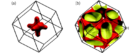
Figure 1: (Color online) Calculated Fermi surfaces (a) and (b) for Nb in first Brillouin zone where the former (latter) is closed (extended).

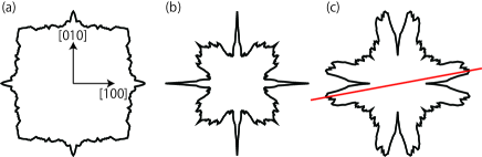
Figure 2: (Color online) The cross sections perpendicular to the field direction H$\parallel$ [001] for the Fermi velocity anisotropy $v_{F}(\theta)$ (a), AR-DOS $D(\theta,\epsilon_{F})$ (b) and the inverse of the AR-DOS (c) where the red line drawn on its maximum direction indicates the lack of the mirror symmetry about this axis tilted by 11^∘ from [100].

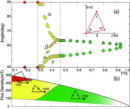
Figure 3: (Color online) Calculated FLL transformation along $H_{c2}$ (a) where the square lattice is tilted by $\delta$=14^∘ from [100], the scalene FLL is stabilized in intermediate $T$, and the isosceles triangle in high $T$ is along [100]. Observed phase diagram in Nb (b).

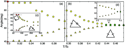
Figure 4: (Color online) Detailed FLL transformation of Fig.1 (a) low $T$ from tilted square to scalene triangle and (b) intermediate $T$ from the scalene to isosceles triangle. The insets (c) and (d) show the experimental datalaver1 for reference: (c) data at 2K as a function of $H$, and (d) data at $H$=200mT as a function of $T$.

Figures 3 and 4 show the FLL transformation along $H_{c2}$ where the unit cell shape characterized by the angles, $\alpha$, $\beta$ and $\gamma$ and the tilting angle $\delta$ from [100] are displayed in Fig. 3(a) and compared with the observed phase diagramlaver1 in $H$ vs $T$ for Nb in Fig. 3 (b). Note that the square lattice tilted by $\delta$=14^∘ is stabilized at the low $T$ and high $H$ region. This tilting angle nearly coincides with the observed value 10.9^∘ and their $H-T$ region also coincides with the observation. Upon increasing $T$, the tilted square lattice changes into the scalene lattice at $t=0.3$. Then after gradual transformation, keeping the scalene nature intact for a finite $H$ region. This scalene lattice that breaks the mirror symmetry of FLL finally gives way to the isosceles triangle lattice at higher $T$. This isosceles is orientated along the [100] direction ($\delta$=0^∘) that coincides with the observation. This lock-in transition occurs smoothly. Upon further increasing $T$, this isosceles triangle lattice tends to the equilateral triangle toward $T_{c}$ smoothly. The overall FFL transformation characterized by the unit cell shape and orientation relative to the crystal lattice along $H_{c2}$ almost perfectly reproduces the observationlaver1 ; laver2 . It should be emphasized that there is no adjustable parameter here and all information on the electronic structures in the normal state, including the Fermi velocity anisotropy and the AR-DOS is coming from the first principles DFT calculations.

In order to understand the physical origins of the remarkable success of the above Eilenberger theory combined with DFT, we construct a minimum model for grasping the essential features of those results. Namely (1) the tilted square at low $T$, (2) the scalene triangle in the intermediate $T$ and (3) the isosceles triangle whose nearest neighbor is along [100] at higher $T$. We model the Fermi velocity anisotropy in the Fermi circle whose radius is $k_{F}$, that is, ${\bf v}_{F}=\beta(\theta)v_{F}^{0}{\bf u}$. $\beta(\theta)$ parametrizes the Fermi velocity anisotropy, and ${\bf u}$ is the unit vector on the plane perpendicular to the field direction. In this model, the AR-DOS is given by $D(\theta,\epsilon_{F})=1/\beta(\theta)v_{F}^{0}$. Namely, the Fermi velocity anisotropy and AR-DOS are not independent quantities as in DFT. We can expand as $\beta(\theta)=\Sigma_{n=0,1,2,\cdots}\beta_{4n}\cos(4n\theta)$. Since it will be clear that $\beta_{4}$ only model cannot account the above features (1)-(3), the minimum model consists of $\beta_{4}$ and $\beta_{8}$. Namely, we consider the following model:

$${\bf v}_{F}(\theta)=v_{F}^{0}{\bf u}\beta(\theta)=v_{F}^{0}{\bf u}(1+\beta_{4}\cos 4\theta-\beta_{8}\cos 8\theta).$$

We have performed extensive calculations based on this model, plugged it into the Eilenberger equation above to find the conditions to reproduce the above features. Then we have found the necessary condition for scalene triangle to appear as $\beta_{8}>\beta_{4}>0$ that also explains the features (1-3) simultaneously.

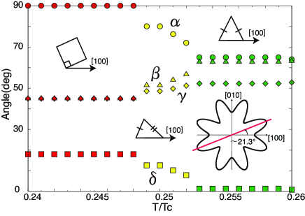
Figure 5: (Color online) FLL transformation based on the minimum model with $\beta_{4}=0.1$ and $\beta_{8}=0.3$. The low $T$ square lattice tilted with 18^∘ from [100] axis transforms into the scalene FLL that is followed by the isosceles FLL at higher $T$ where the nearest neighbor orients along [100] direction.

Figure 5 shows an example for this case ($\beta_{4}=0.1$ and $\beta_{8}=0.3$). In the lowest $T$ region, the square lattice appears with the tilting angle $\theta=18^{\circ}$ while the Fermi velocity maximum is at $\theta=21.3^{\circ}$. There is a rule that at lower $T$ the stable square lattice is oriented along either the AR-DOS maximum for isotropic gap case or the nodal direction for d-wave gap casesuzuki .

Then by increasing $H$, the tilted square deforms continuously into the scalene triangle FLL as seen from Fig. 5 in the middle $T$. This scalene lattice is locked-in the isosceles triangle lattice oriented along [100]. Those sequences of the FLL transformation are same as in DFT case above. It is now clear that the essential ingredient for the scalene triangle to appear is the lack of the mirror symmetry about the Fermi velocity maximum direction as indicated in the inset of Fig. 5 and also note that in Fig. 2(c) the inverse of AR-DOS also shows this. This velocity maximum simultaneously explains why the square lattice is tilted. Namely the tilted square FLL and scalene FLL are intimately tied with each others. Note that while our $\beta_{4}$-$\beta_{8}$ minimum model explains the appearance of the scalene FLL, the stable $T$ region is far off the observation.

In order to understand the origin of the scalene FLL, we display the deformation of this lattice in Fig. 6(a). It is seen from it that the deformation occurs so that one of the two diagonal axes of the parallel piped unit cell continuously rotates, keeping the other axis intact. This movement can be interpreted as the scalene FLL seeks stable configuration by adjusting the unit cell angle and its orientation by utilizing the possible freedoms allowed. As a result of the broken mirror symmetry about the velocity maximum direction the scalene FLL could appear. This situation is quite different from that in the $\beta_{4}$ only (the same for the $\beta_{8}$ only model) where the mirror symmetry is preserved in the velocity anisotropy along the maximum direction. As shown in Fig. 6(b), the FLL deformation from the square to isosceles triangle proceeds as follows: The two diagonal axes of the parallel piped unit cell keep unchanged, always orthogonal with each other and the two angles of the isosceles continuously changes.

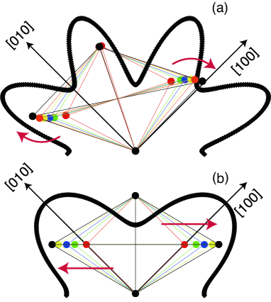
Figure 6: (Color online) FLL transformations as $T$ increases for the two cases where the bold curves are the Fermi velocity anisotropies: (a) FLL changes from the square to the scalene for the minimum model with $\beta_{4}=0.1$ and $\beta_{8}=0.3$. (b) FLL changes from the square to the isosceles for $\beta_{4}=0.1$ where the mirror symmetry is unbroken about the maximum direction [100].

It is important to notice that one of the two diagonal axes is kept to point along the direction of the velocity minimum during the deformation. In other words, the base of the isosceles is always kept along the velocity minimum direction. The pairs of the vortices on the unit cell move along those symmetry constraint axes, preserving the mirror symmetry. This is contrasted with the present scalene case where the two diagonal axes rotate each other, thus no symmetry constraint during the deformation because the mirror symmetry about the maximum direction is broken from the outset. Comparing the two cases with either broken mirror symmetry or with unbroken symmetry, it is concluded that a necessary condition, but not sufficient condition for the scalene triangle FLL to occur is that in the anisotropic velocity the mirror symmetry is broken about the anisotropy maximum direction. The broken mirror symmetry of the FLL that is real space is originated from the mirror symmetry breaking in the reciprocal space. Furthermore, it is interesting to notice the experimental fact that the appearance of the scalene FLL is tied with the appearance of the tilted square lattice in Nb. As mentioned above, the square FLL is oriented along the velocity maximum direction at lower $T$, that is a general theoretical fact within our model calculations. Thus, in Nb the Fermi velocity maximum is situated along the direction tilted by 11^∘ from the [001] axis and the mirror symmetry about this axis must be broken.

In summary, we demonstrate that the first principles band calculation combined with microscopic Eilenberger analysis yields an excellent explanation of the observed FLL transformation in Nb under $H\parallel[001]$, including the tilted square and scalene lattices without adjustable parameter. This opens a door that this combined method provides a fundamental framework to truly understand the vortex matter from first principles. We also show the possible reasons why the spontaneous mirror symmetry is broken in the scalene lattice by constructing a minimum model for the Fermi velocity anisotropy.

We thank M. Laver and E. M. Forgan for stimulating discussions. We also acknowledge useful discussion with P. Miranovic. This work is partly performed during a stay in Aspen Center for Physics.

References

- (1) See for example, E. Hand, Nature 456, 555 (2008). G. Catelani and J. P. Sethna, Phys. Rev. B 78, 224509 (2008).
- (2) M. Laver, et al., Phys. Rev. Lett. 96, 167002 (2006).
- (3) M. Laver, et al., Phys. Rev. B 79, 014518 (2009).
- (4) S. Mühlbauer, et al., Phys. Rev. Lett. 102, 136408 (2009).
- (5) M. Laver and E. M. Forgan, Nature Commun. 1, 45 (2010).
- (6) H. W. Weber, Anisotropy Effects in Superconductors (Plenum Press, New York, 1977).
- (7) A. D. Bianch, et al., Science 319, 177 (2008).
- (8) T. M. Riseman, et al., Nature 396, 242 (1998).
- (9) R. Gilardi, et al., Phys. Rev. Lett. 88, 217003 (2002).
- (10) M. R. Eskildsen, et al., Phys. Rev. Lett. 78, 1968 (1997).
- (11) M. R. Eskildsen, et al., Phys. Rev. Lett. 79, 487 (1997).
- (12) L. Debeer-Schmitt, et al., Phys. Rev. Lett. 99, 167001 (2007).
- (13) K. Takanaka, Prog. Theor. Phys, 50, 365 (1973).
- (14) T. Kita and M. Arai, Phys. Rev. B 70, 224522 (2004).
- (15) Y. Nagai, H. Nakamura and M. Machida, Phys. Rev. B 83, 104523 (2011).
- (16) G. Eilenberger, Z. Phys. 214, 195 (1968).
- (17) M. Ichioka, et al., Phys. Rev. B 55, 6565 (1997). M. Ichioka and K. Machida, Phys. Rev. B 65, 224517 (2002).
- (18) N. Nakai, et al., Phys. Rev. Lett. 89, 237004 (2002).
- (19) P. Blaha, K. Schwarz, G. Madsen, D. Kvasnicka and J. Luitz, WIEN2k (Vienna Univ. Technology, Austria, 2001).
- (20) T. Kita, J. Phys. Soc. Jpn., 67, 2067 (1998).
- (21) K. M. Suzuki, et al., J. Phys. Soc. Jpn., 79, 013702 (2010).
- (22) L. F. Mattheiss, Phys. Rev. B 1, 373 (1970).