Simulation of a strategy for the pixel lensing of M87 using the Hubble Space Telescope

Abstract

In this work we propose a new strategy for the pixel-lensing observation of M87 in the Virgo cluster using the Hubble Space Telescope (HST). In contrast to the previous observational strategy by Baltz et al., we show that a few days intensive observation with the duration of $\sim 90~{}$min in each HST orbit will increase the observational efficiency of the high-magnification events by more than one order of magnitude. We perform a Monte-Carlo simulation for this strategy and we show that the number of high magnification microlensing events will increase at the rate of $4.2$ event per day with a typical transit time scale of $16$ h. We also examine the possibility of observing mini-halo dark matter structures using pixel lensing.

Key words:gravitational lensing:Micro-dark matter-galaxies:M87

1 introduction

One of the consequence of Einstein General Relativity is that light is deflected by the gravitational field of an object with an angle of

$$\alpha=\frac{4GM}{c^{2}b},$$ (1)

where $M$ is the mass of the deflector and $b$ is the impact parameter of the light ray Einstein (1911). In the case of lensing of a background star by another star, this deflection creates extra images of a background object where the images are too close to be resolved by the ground-base telescopes. This type of lensing is called gravitational microlensing. In 1936, Einstein said ”there is a little chance of observing gravitational lensing caused by the stellar mass lenses”. However, after several decades, using advanced cameras and computers, and following the propose of Paczyński (1986), the first microlensing event has been discovered by Alcock et al. (1993).

The aim of the microlensing observational groups such as MACHO, EROS and OGLE Alcock et al. (2000); Afonso et al. (2003); Wyrzykowski et al. (2009) has been to monitor stars the Large and the Small Magellanic Clouds in order to detect the massive compact halo objects (MACHOs) of the halo using gravitational microlensing. The passage of the MACHOs from the line of sight of the background stars causes an achromatic magnification of the background stars with a specific shape. Comparing the number of the observed events with that expected from the halo models have shown that MACHOs made up less than 20 per cent of the Galactic halo Milsztajn & Lasserre (2001); Rahvar (2004); Moniez (2010). They can not cover all the dark matter budget of the halo. In this paper, we question further the existence of MACHOs on cosmological scales, and suggest a strategy for observation using the Hubble Space Telescope (HST).

Gravitational microlensing towards the source stars beyond the Galactic halo can be performed with an observational method - so-called pixel lensing- which is different to the conventional method. When the background stars are too far and the field is too dense to be resolved, using this method a high magnification microlensing event can change the light flux in each pixel. By recording the time variation of the light in each pixel, it is possible to recognize a microlensing event Crotts (1992); Baillon et al. (1993). An important factor for increasing the sensitivity of the observations when using the pixel lensing is the size of point spread function (PSF). Several groups as MEGA, AGAPE and ANGSTROM, have monitored M31. They have found few pixel-lensing candidates in this direction Crotts & Tomaney (1996); Ansari et al. (1999); Kerins et al. (2006).

Gould (1995) proposed the extension of pixel lensing to cosmological scales, using the observation by the HST towards the Virgo cluster. He proposed an investigation of the intercluster MACHOs and obtained a theoretical optical depth of $\tau\sim 3\times 10^{-5}f$, where $f$ is the fraction of halo composed of MACHOs Gould (1995). The detection threshold of an event was defined by the accumulation of the signal to noise of the events for the duration that an event is observable. So, in this observation, one would expect to detect microlensing events with a long duration and a low peak in light curve. The estimation obtained for the rate of events with this observational threshold was $\Gamma\sim 18f~{}day^{-1}$. Baltz et al (2004) used the HST for pixel lensing and monitored M87 for one month, using with the strategy of taking one date point per day. After data reduction, seven candidates remained. With further investigation of the light curves in two different colors they concluded that one candidate could be a microlensing event. Comparing the observational result with the expectation from generating synthetic light curves, they concluded that the fraction of MACHOs in both the Milky Way and the Virgo halos are almost equal Alcock et al. (2000). However, the problem with this statistical analysis is that one microlensing event has a large statistical uncertainty. In order to have a better estimation of the MACHOs in the Virgo cluster, we need to be observed more events.

In this work we extend the work by Gould (1995) and Baltz et al. (2004), and we propose an alternative observational strategy using the HST. Our suggestion is to observe the very high magnification events in M87, which has a variation in its light curve in the order $1$ d. In order to improve the sensitivity of observing of short duration events, we need to increase the sampling rate by the order of $1$ h. We propose intensive short-duration observation of M87 of the order of $1$ h using the Wide Field Planetary Camera 3 (WFC3) of the HST. We suggest taking one date point in each orbit and collecting about $15$ photometric data point per every $24$ h. This strategy will enable us to detect very high magnification short-transit pixel lensing events.

First, we make a rough calculation to estimate the optical depth and the detection rate of the events using this observational strategy. In order to have a better estimation, we continue with a Monte-Carlo simulation for three observational programs of $1$, $2$ and $3$ d. We examine how sensitivity the results are to the duration of the observational program. We show that with $1$, $2$ and $3$ d of intensive observation with the HST, it is possible to detect $4.2$, $13.4$ and $18.5$ events per day, respectively. We also simulate the observation using the strategy of Baltz et al. (2004), with the cadence of $1$ d, and find $0.02$ event per day for one month observations.

The paper is organized as follows. In section 2, we introduce the Virgo cluster and obtain the theoretical optical depth and the event rate of the high magnification events from structures along the line of sight. In section 3, we perform a Monte-Carlo simulation to obtain the number of the high- magnification events found with the HST. The results are given in section 4. In section 5 we give our conclusion.

2 pixel lensing of M87

Virgo cluster contains $\sim 1300$ galaxies and is located about $16.5$ Mpc from us. It has am apparent size of $8^{\circ}$ and coordinate of RA$\sim 12~{}hrs$ and DE$\sim 12^{\circ}$ Fouqué et al. (2001); Mei et al. (2007). The brightest galaxy of this cluster is M87 which is located at the center of this structure. Similar to the Local Group, the mass of the Virgo cluster is mainly made up of dark matter. With microlensing of the Virgo cluster, it could be possible estimate the fraction of MACHOs in the halo of this structure.

Because stars in the Virgo cluster cannot be resolved using present ground- and space- based telescopes, the standard microlensing technic cannot be used for the stars in the Virgo cluster. To make an estimation from the column density of the stars, we assume that galaxies in the Virgo cluster have the same surface density of stars as in the Milky way, ($\Sigma=50M_{\odot}/pc^{2}$). For HST with a PSF size of $0.067$ arcsec in the WFC3, the number of stars inside the PSF would be about $1000$ Drive (2010). To detect a microlensing event in a high blended background, we need a very high magnification event to change the flux of pixels inside the PSF. In what following, we provide a rough estimation from the optical depth and the event rate in terms of the transit time towards M87. In Section 3, we obtain a precise value of the event rate, based on a Monte Carlo simulation using HST observations.

The standard definition of the optical depth is the cumulative fraction of area covered by the Einstein ring for all the distances from the observer to the source star Paczyński (1986):

$$\tau=\int_{0}^{D_{s}}\frac{\rho(D_{l})}{M}\pi R_{E}^{2}dD_{l},$$ (2)

where $R_{E}$ is Einstein radius, $M$ is the typical mass of the lens, $\rho(D_{l})$ is the mass density of the lens and $D_{l}$ is the distance between the observer and lens.

Taking M87 as the target galaxy, the column density of stars at the center of this galaxy is much larger than that at the edge of the galaxy. Thus, the threshold for detecting a very high magnification event would depend on the position of the source star in M87. Assuming a spherical model for M87, we calculate the column density of the stars by integrating the number density of stars along the line of sight, $\Sigma(r)=\int n(r,z)dz$. Then, the number density of stars for a given solid angle would be $dN/d\Omega=D^{2}\Sigma$. The number of stars inside the PSF is given by $\Delta N_{PSF}=dN/d\Omega\times\Omega_{PSF}$. Fig. (1) plots the number of stars inside the PSF in terms of separation from the center of the galaxy in arcsec, using the galaxy model in McLaughlin (1999).

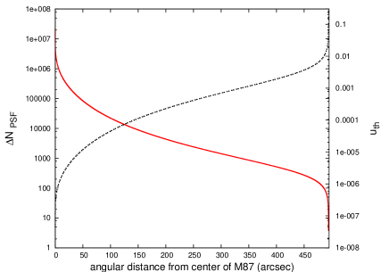
Figure 1: Number of stars inside the PSF size (solid line) indicated at the left hand side of y-axis and threshold for the impact parameter (dashed-line) indicated at the right hand side as a function of angular distance from the center of the galaxy.

The threshold impact parameter can be defined according to the blending inside the PSF. Because the threshold magnification should be more than the number of stars inside the PSF (i.e. $A_{th}>\Delta N_{PSF}$), the corresponding threshold for the impact parameter can be defined as $u_{th}<(\Delta N_{PSF})^{-1}$. Fig. 1 shows the threshold impact parameter as a function of the angular separation from the center of the galaxy, as indicated by the dashed line.

We can define a new optical depth according to the threshold impact parameter in such a way that $\tilde{R}_{E}=u_{th}R_{E}$. Using the definition of the optical depth based on this reduced Einstein radius, this relates to the conventional definition of optical depth as follows:

$$\tilde{\tau}(\hat{n})=u_{th}^{2}(\hat{n})\tau(\hat{n}),$$ (3)

where, $\hat{n}$ is the direction of the observation and $\tau$ is the standard definition of the optical in equation (2). In what follows, we estimate the numerical value of the standard optical depth, resulting from the various structures along the line of sight. Finally, we obtain the optical depth of the observable high-magnification events by multiplying the optical depth by the threshold impact parameter, as in equation (3). We note that the lenses along the line of sight can be in the halo of Milky Way, the disc of the Milky Way, the halo of the Virgo cluster, the halo of M87 or M87 itself. We calculate the optical depth towards all area of M87 and we provide the average optical depth of each structure, as follows.

(i) We assume lenses in the galactic disc as the nearest structure to the observer. The mass density for the lenses is given by Binney & Tremaine (1987)

$$\rho(R,z)=\frac{\Sigma}{2H}\exp\left[-\frac{(R-R_{\odot})}{h}\right]\exp\left(-\frac{|z|}{H}\right).$$ (4)

Here, $h$ is the length-scale of the disc, H is the height-scale and $\Sigma$ is the column density of the disc at the position of the sun, $R_{\odot}$. Substituting $\rho(R,z)$ into the equation (2) and integrating over $D_{l}$, the average value of the optical depth weighted by the number of background stars over M87, we obtain $\tau_{i}\sim 1.4\times 10^{-9}$.

(ii) For the Galactic halo, we use NFW mass density profile Navarro et al. (1996)

$$\rho(r)=f_{h}\frac{\delta_{c}\rho_{c}}{(r/r_{s})(1+r/r_{s})^{2}},$$ (5)

Here, $r_{s}$ is the characteristic radius, $\rho_{c}={3H_{0}^{2}}/{8\pi G}$ is the present critical density, $f_{h}$ is the fraction of halo composed of MACHOs, $r$ is the position of the lens from the center of galaxy and $\delta_{c}=200c^{3}g(c)/3$, where $c$ is the concentration parameter and

$$g(c)=\frac{1}{\ln(1+c)-c/(1+c)}.$$

We set $c=18$ and $r_{s}=14kpc$ for galactic halo Battaglia et al. (2005). We obtain the average optical depth from this structure $\tau_{ii}\sim f_{h}\times 1.1\times 10^{-6}$, which is three order of magnitude larger than that of the Galactic disc.

(iii) The third structure is the halo of Virgo cluster. We set the NFW parameters for the Virgo halo as $r_{s}\sim 560kpc$ and $\delta_{c}\rho_{c}=3.2\times 10^{-4}M_{\odot}/pc^{3}$McLaughlin (1999). The optical depth is obtained as $\tau_{iii}\sim f_{v}\times 3.38\times 10^{-5}$, where $f_{v}$ is the fraction of Virgo halo composed of MACHOs. We note that the optical depth from the Virgo cluster is also one order of magnitude larger than the Galactic halo.

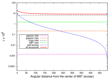
Figure 2: The optical depth towards the Virgo cluster in terms of the transverse angular separation from the center of the cluster for various structures. The solid line is the overall optical depth by accumulating the result from the different structures.

(iv) The lens can reside in the galactic halo of M87. We take the NFW model for the halo of this structure with the parameters of $r_{s}=50kpc$ and $c=15$ Gebhardt & Thomas (2009); Doherty et al. (2009). The optical depth resulting from this structure is $\tau_{iv}\sim f_{M87}\times 7.62\times 10^{-6}$.

(v) Finally, the lens can be in M87, so-called self-lensing events. We assume M87 is located at the center of the Virgo cluster with a spherical shape and a radius size of $40kpc$ Gebhardt & Thomas (2009). For this structure, we use the mass density profile of McLaughlin (1999):

$$\rho(r)=\frac{3-\gamma}{4}\frac{\Upsilon_{B}L_{B}}{\pi a^{3}}\left(\frac{r}{a}\right)^{-\gamma}\left(1+\frac{r}{a}\right)^{(\gamma-4)},$$ (6)

where $\gamma=1.33$, $a=5.1\pm 0.6~{}kpc$, $L_{B}=(5.55\pm 0.5)\times 10^{10}~{}L_{\odot,B}$, $\Upsilon_{B}=14.6\pm 0.2~{}M_{\odot}L_{\odot,B}^{-1}$ and $r$ is the distance from the center of M87. The optical depth resulting from the self-lensing is $\tau_{v}\sim 1.73\times 10^{-6}$.

We note that the halo of Virgo has the highest contribution in the optical depth towards M87. Fig. (2) shows the optical depth resulting from the various structures as a function of angular separation from the center of the galaxy. Knowing the optical depth and the threshold impact parameter, we use the definition of the reduced optical from equation (3) and we obtain $\tilde{\tau}$ in terms of angular distance from the center of M87 by multiplying the standard definition of the optical depth in Fig.(2) by $u_{th}^{2}(\theta)$ from Fig. 1. The result is shown in Fig.3. We summarize the result of the reduced optical depth in Table 1. Here, we assume that MACHOs contribute $20$ per cent of the halo mass.

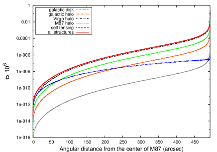
Figure 3: The reduced optical depth as a function of angular distance from the center of M87, resulting from the multiplication of the optical depth to the square of threshold impact parameter, i.e. $\tilde{\tau}(\theta)=\tau(\theta)u_{th}^{2}(\theta)$.

We note that, in contrast to the standard definition of the optical depth, which is almost constant for all the directions towards the target structure, the reduced optical depth depends on the line of sight towards M87. It is small at the center of M87 and becomes larger at the edge of the structure.

		a	b	c	d	e	overall
	$\tilde{\tau}\times 10^{11}$	0.00074	0.118	3.622	0.819	0.0028	4.563
	$t_{1/2}(hr)$	6.11	5.39	17.32	9.02	32.26	15.85
	$N_{e}(1/day)$	0.0032	0.607	5.794	2.513	0.013	8.93

Table 1: Reduced optical depth (first row), transit time (second row) and the number of the events (third row) for each structure. Structures in each column are noted by (a) Galactic disk; (b) Galactic halo; (c) Virgo halo; (d) M87 halo; (e) self lensing and last column is mean value for the optical depth and transit time and the the overall number of detected events per day.

From the definition of the optical depth, we can obtain the rate for events for those with the impact factor smaller than $u_{th}$. From the dependence of the number of events on the optical depth, the rate of events is obtained as

$$\frac{N_{e}}{T_{obs}N_{bg}}=\frac{2}{\pi}\frac{\tilde{\tau}}{\tilde{t}_{E}},$$ (7)

Here, $N_{e}$ is the number of the observed events, $N_{bg}$ is the number of the background stars during the observational time of $T_{obs}$ and the reduced Einstein crossing time is defined as $\tilde{t_{E}}=u_{th}t_{E}$. Using the definition of $\tilde{\tau}$, the rate of events can be written in terms of the optical depth and the Einstein crossing time as

$$\frac{N_{e}}{T_{obs}N_{bg}}=\frac{2}{\pi}\frac{\tau}{t_{E}}u_{th}.$$ (8)

One of the relevant time scales in the high-magnification microlensing events is ${t}_{1/2}$, which is defined as the full width at half-maximum (FWHM) timescale of the high magnification events. For high magnification events, the magnification changes with the impact parameter as $A=1/u$. The transit time for these events relates to the Einstein crossing time as $t_{1/2}=2\sqrt{3}u_{0}t_{E}$. Hence, for each event, after fitting the observational light curve with the theoretical light curve, we can obtain $t_{1/2}$ in terms of $u_{0}$ and $t_{E}$. Finally, taking the number density of background stars $dN(\theta)_{bg}/d\Omega$ as a function of angular distance from the center of the structure, we can obtain the differential rate of events as

$$\frac{dN_{e}}{T_{obs}d\theta}=\frac{4dN_{bg}(\theta)}{d\Omega}\frac{u_{th}(\theta)\tau(\theta)}{t_{E}(\theta)}\theta.$$ (9)

Using this equation and the estimation for the time-scale of $t_{E}$, we obtain the rate of events as shown by the solid line in Fig.(4) in terms of the angular distance from the center of M87. Integrating over $\theta$ results in the number of the detectable events. Here, we obtain about $\sim 9$ high magnification microlensing events per day. We note that in this rough estimation, we did not use the quality of light curve on delectability of the events. Also we ignored the finite-size effect on the detections made with pixel lensing. In the section 3, we will re-analyse and simulate the light curves of M87 using the HST. Table (1) reports the reduced result of this preliminary analysis and provide the reduced optical depth from the various structures, $t_{1/2}$ and and the rate of the events.

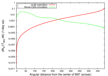
Figure 4: The event rate as a function of angular distance from the center of M87. The solid line is obtained from the rough calculation and the dashed line shows the result from the Monte-Carlo simulation.

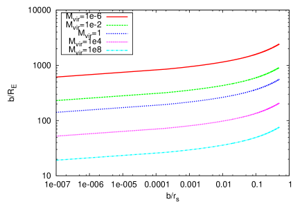
Figure 5: The impact parameter normalized to the Einstein radius for micro-halos in terms of the impact parameter normalized to the size of micro-halo for the structures with various masses.

Finally we examine the possibility of observing dark matter micro-halo structures Goerdt et al. (2007); Erickcek & Law (2010) using pixel lensing. Taking the NFW profile for these structures, in order to have high- magnification events from these lenses, we have to decrease the impact parameter down to $\sim 10^{-3}$. The problem with dark halo structures is that the mass of the structure enveloped by sphere with the radius of the impact parameter decreases towards the center of structure. Fig. (5) plots the impact parameter normalized to corresponding Einstein radius in term of the impact parameter normalized to the size of the structure. For microhalos, the normalized impact parameter, $b/R_{E}$ is always larger than one and never reach below $10^{-3}$, a favorable value for the pixel lensing. Our conclusion is that we can ignore possible contribution of these structures in pixel lensing. With current technology, it is not possible to detected the micro-halo structures.

3 MONTE-CARLO SIMULATION

In this section we perform a Monte-Carlo simulation to obtain the detection efficiency and the rate of microlensing events towards M87 using pixel lensing. In the first step, we simulate the stellar distribution in M87, using the color-magnitude profile of the stars of the galaxy. Then, we use the foreground structures to obtain the distribution of the lenses along the line of sight. In the pixel lensing, the magnification is suppressed by the blending and the finite size effect. We take into account these two effects in our simulation.

To simulating the stellar distribution in M87, we use the theoretical Isochrones of the color-magnitude diagram diagram (CMD) obtained using the numerical simulation of the stellar evolution from the Padova model Marigo et al. (2008). The Isochrones are defined for the stars with different mass, color, magnitude but with the same matalicity and age. To simulating the CMD, we select isochrones with the metalicity range of $Z=0.0004,0.008,0.004,0.001,0.019$ and $0.030$. For the evolution of the stars, we take the ages of the stars in the range of $log(t/yr)=[6.6,10.2]$ with interval of $\bigtriangleup log(t)=0.05$ dex. For each age range, we take a metalicity according to the age-metalicity relation, and the distribution function for the metalicity from Twarog (1980). In order to generate the CMD of the stars at the present time, we need an initial mass function of the stars and the star formation rate function for M87. The initial mass function is chosen from the Salpeter function Salpeter (1995). For the star formation rate, we assumed a positive rate $dN/dt>0$ similar to that in our Galaxy Cignoni et al. (2006); Karami (2010). The result of our simulation in the absolute CMD is shown in the left panel of Fig.(6).

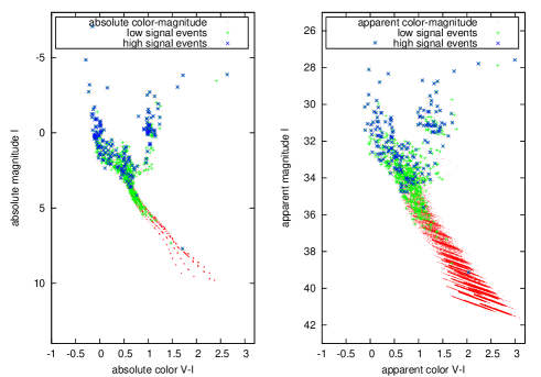
Figure 6: CM diagram generated by Padova Isochrones. The left panel is the absolute color–magnitude diagram and the right panel is the apparent CM generated according to the distance modulus, extinction and reddening of the stars. We show a sample of microlensed stars with a high signal to noise of $Q=30$ (cross sign) and low signal to noise of (plus sign) $Q=5$ in the Pixel lensing.

In order to generate the apparent color-magnitude of the stars, we calculate the distance modulus of each star in M87 and add it to the corresponding extinction. Because dust in the interstellar medium is proportional to the Hydrogen density, we can use the column density of hydrogen $(N_{H})$ along the line of sight as an indicator of amount of extinction. For the $V$ and $I$ bands, the amount of extinction is given by Weingartner & Draine (2001):

$$A_{V}(mag) = 5.3\times 10^{-22}N_{H}(atom/cm^{2}),$$

$$A_{I}(mag) = 2.6\times 10^{-22}N_{H}(atom/cm^{2}).$$ (10)

For the distribution of the hydrogen in M87, we choose the theoretical distribution function of hydrogen, which has the best fit to the X-ray observation Tsai (1994):

$$n_{e}(r)=n_{0}\frac{(r/a_{1})^{-\alpha}}{1+(r/a_{1})}.$$ (11)

Here, $a_{1}=9.51kpc$, $\alpha=0.36$, $n_{0}=3.51\times 10^{-2}atom/cm^{3}$ and $r$ is the distance from the center of the structure.

Finally, the apparent magnitude and color of each star are given by

$$m_{V} = M_{V}+5\log\left[\frac{d(pc)}{10}\right]+A_{V},$$

$$C_{obs} = C_{0}+A_{V}-A_{I},$$ (12)

Here, $C_{0}$ is the absolute color, $M_{V}$ is the absolute magnitude in the visible band and $d$ is distance of stars in parsec. We plot the apparent color-magnitude of the stars of M87 in the right panel of Fig.(6), including the effect of the distance modulus, extinction and the reddening.

			a	b	c	d	e	overall
	1	$\tau\times 10^{6}$	0.00139	0.219	6.758	1.525	1.734	10.238
	2	$N_{e}(1/day)$	1.2e-6	0.0022	4.2	0.018	0.0072	4.2
			a	b	c	d	e	average
	3	$\rho_{\star}/u_{0}$	0.002	0.16	1.5	6.2	1.3	1.5
	4	$t_{1/2}(hr)$	12.6	15.6	16.9	5.6	4.5	16.3
	5	$A_{max}$	447.9	688.9	319.8	509.7	537.9	348.4
	6	$u_{0}$	0.004	0.007	0.032	0.003	0.0038	0.029
	7	$m(mag)$	31.3	30.4	29.6	31.1	32.2	29.7

Table 2: Result from the simulation of one day observation by the HST with the WFC3 camera. The columns are (a) Galactic disk;(b) Galactic halo; (c) Virgo halo; (d) M87 halo; (e) self lensing. The first and second row represents the optical depth and the number of the events resulting from each structure and the last column indicates the overall numbers. The third line is the mean value of $\rho_{\star}/u_{0}$ for the observed events in each structure. The forth row represents the average transit time scale of the events, the fifth row is the average of maximum magnification, the sixth row is the impact parameter and the seventh row is the apparent magnitude of the source stars. The last column represents the average value for the parameters of the lenses.

In the next step, we generate the light curve of the microlensing events by choosing the parameters of the lens as the mass, the velocity and the location, according to the corresponding distribution functions. The location of the lenses from the observer is calculated according to the probability function for the location of lenses

$$d\Gamma/dx\propto\rho(x)\sqrt{x(1-x)}$$

, where $x=D_{l}/D_{s}$ and $\rho(x)$ is the mass density profile of the lenses along the line of sight. The mass of the lenses, in units of solar mass, are chosen from the Kroupa mass function Kroupa et al. (1993); Kroupa (2001), $\xi\propto M_{l}^{-\alpha}$, where $\alpha=0.3$ for $0.01\leq M_{l}<0.08$, $\alpha=1.3$ for $0.08\leq M_{l}<0.5$ and $\alpha=2.35$ for $0.5\leq M_{l}\leq 1.0$. The velocity of lenses in the halo is chosen from the Maxwell-Boltzmann distribution with the dispersion velocity indicated by the Virial theorem. For the Galactic halo, the Virgo halo and the M87 halo, the dispersion velocities are set as $\sigma\sim 156~{}kms^{-1},1000~{}kms^{-1}$ and $350~{}kms^{-1}$, respectively Dehnen et al. (2006); Gebhardt & Thomas (2009). The distribution for velocity of stars in the Galactic disc is also chosen from ellipsoid of the dispersion velocity Binney & Tremaine (1987). The velocity of stars in M87 is chosen from Maxwell-Boltzmann function with $\sigma\sim~{}360kms^{-1}$ Romanowsky & Kochanek (2001). The minimum impact parameter $u_{0}$ in this simulation has to be chosen geometrically uniform in the range of $u_{0}\in[0,1]$. However, in the Monte-Carlo simulation, we generate a uniform impact factor in the logarithmic scale to have enough statistics of the high- magnification events and to reduce the computation time. In order to recover the uniform distribution of impact parameter, we consider a weight proportional to the impact parameter $u_{0}$ when counting the number of events.

To calculate the finite-size effect, we need the size of the stars projected on the lens plane. For the main-sequence source stars, the radius of the stars is obtained according to the mass–radius relation as

$$R_{\star}=M_{\star}^{0.8}.$$ (13)

Here, the parameters are normalized to the Sun’s values. Red giants (RGs) also follow the relation of Hayashi et al. (1962)

$$M_{RG}^{1/2}R_{RG}^{3/2}=const.$$ (14)

The formalism of the finite-size effect in the gravitational lensing was obtained by Maeder mae73 (1973) and developed later for microlensing by Witt & Mao wit (1994). The relevant parameter in the finite size effect is $\rho_{\star}/u_{0}$, where $\rho_{\star}$ is the projected radius of the star on the lens plane normalized to the Einstein radius. For the population of the source stars in M87 and lenses in various structures along the line of sight, Table (2) gives the average value of $\rho_{\star}/u_{0}$, with the corresponding $\rho_{\star}$ and $u_{0}$ for the observed events in each structure. We examine the finite-size effect on the main sequence and RG stars. We find that $43\%$ per cent of stars with an absolute magnitude less than zero are RG, but for the microlensed stars in this range only $17$ per cent are RGs.

In the pixel lensing, because of the high blending in each pixel, the signal to noise ratio from microlensing must be so high to be distinguishable from the background brightness of the host galaxy. For a background star with the apparent magnitude of $m$, the extra photons during the magnification of the star are obtained by

$$\delta N=(A-1)\times t_{exp}\times 10^{-0.4(m-m^{zp})}.$$ (15)

Here, $A$ is magnification factor of the source star, $t_{exp}$ is exposure time and $m^{zp}$ is the zero-point magnitude equivalent to the flux $=1$ photoelectron^-1, which is equal to $25.10$ and $26.08$ mag in I-band (F814W) and V-band (F606W), respectively, for the WFC3 camera of the HST. We note that the observation by Baltz et al. (2004) were performed with the WFC2, which had a lower zero-point magnitude of $23.86$ mag for the I band. The exposure time can be obtained from the visibility of M87 by HST. For M87, which is located at $DEC=12^{\circ}$, the visibility would be about $52~{}$min in each HST orbit. We use the I-band (F814W) filter for observation in the simulation. We show that the background events, such as novas, cannot pass our light curve criterion for a short observation period. Thus, we do not use another filter, such as the R band, for the variable identifer and devote all the observation time in the I band to increase the signal-to-noise ratio. Within each orbit, we assume six $260~{}$s exposure with an overall exposure of $1560~{}$s in I band. The noise is considered as the intrinsic Poisson fluctuation inside the PSF. This is proportional to the square of the number of the photons received from the background sky and the host galaxy:

$$\sqrt{N}=10^{0.2m^{zp}}\sqrt{\Omega_{PSF}(10^{-0.4\mu}+10^{-0.4\mu_{sky}})t_{exp}},$$ (16)

Here, $\Omega_{PSF}$ is the characteristic area of the PSF, $\mu_{sky}$ is the brightness of the background sky (set to $21.6mag~{}as^{-2}$ and $\mu$ is the surface brightness profile of M87. In our Monte-Carlo simulation, we accept the events with the following criterion:

$$Q=\sqrt{\sum_{i}(\delta N_{i}/\sqrt{N})^{2}}>Q_{crit}.$$ (17)

Here, the summation is performed over the observed points of the light curve Gould A. (1996) and $Q_{crit}$ is the critical value for the signal-to-noise of the detection (chosen to be $Q_{r}=5$ for a relaxed criterion and $Q_{s}=30$ for a strict criterion). The $Q^{2}$ is equivalent to the $\chi^{2}_{bl}$ fit of the light curve to the baseline.

As the second criterion, we adopt those events in which the peak of the light curve resides within the duration of the HST observation, (i.e. $t_{0}\in[0,T_{obs}]$, means that we detect events with both rising and declining parts of the light curve). For the short term events, the probability of fulfilling this criterion is higher than for the long duration events. We add another criterion, which is sensitive to the fast variation of the light curve, for which we detect at least three consecutive data points, $3\sigma$ above the background flux. This means that we have, at least, a $3\times 3\sigma$ deviation of the microlensing light curve from the bassline fit. In other words, the difference between the two different fits should be at least $\Delta\chi^{2}=\chi^{2}_{bl}-\chi^{2}_{ml}>27$.

In Fig.(6), we identify the observed events that result from the simulation in the CMD using ${}^{\prime}+^{\prime}$ symbols for the relaxed criterion and ${}^{\prime}\times^{\prime}$ symbols for the strict criterion. We also plot a typical simulated light curve for a high-magnification microlensing event in Fig.7. The error bars are $1\sigma$ results from the Poisson fluctuations in the number of photons received by the detector, according to equation (16), shifted by a Gaussian function from the theoretical light curve. The top panel of the Fig. 7 represents the peak of the theoretical light curve and the simulated data points with the duration of $\sim 90~{}min$. The whole light curve is shown in the bottom panel. Similar to the distribution of $t_{E}$ towards a given source, we plot the distribution of the relevant transit time of $t_{1/2}$ in Fig. 8. The overall number of the events are normalized according to Table 2.

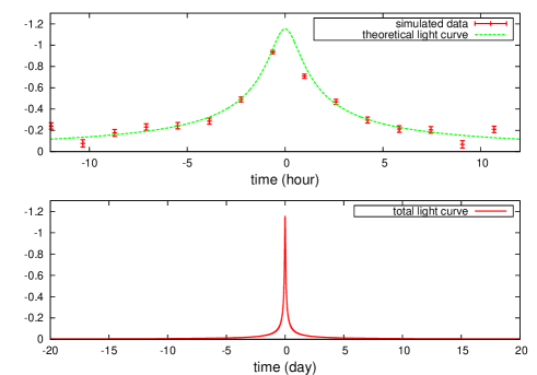
Figure 7: The theoretical light curve of a high magnification microlensing event including the blending of the background stars with the simulation of the observation with the cadence of $\sim 90~{}min$ (top panel data points). In the bottom panel we show the same event for the duration of $40$ days.

One of the backgrounds that we should take into account in the simulation of the light curves is the hot pixels of the CCD resulting from the cosmic rays. The probability of a hot pixel in the HST for $1000~{}s$ exposure time is $1.5\sim 3\%$ Sirianni et al. (2005). We take into account the effect of cosmic rays and discard the hot pixels from the light curve. The other backgrounds that can be mistaken for a microlensing events are the variable stars and novas. The annual average Novas in M87 is about $\sim 64$ Madrid et al. (2007). So, during the observations over 1 or 2 d, we can expected one event, at most, to be detected. Also, the variable stars do not have enough variation in the light curve to be detected in the high blending medium. We ignore the effects of novas and variable stars.

Figure 8: The distribution function of $t_{1/2}$ of the observed events with the criterion of $Q>5$.

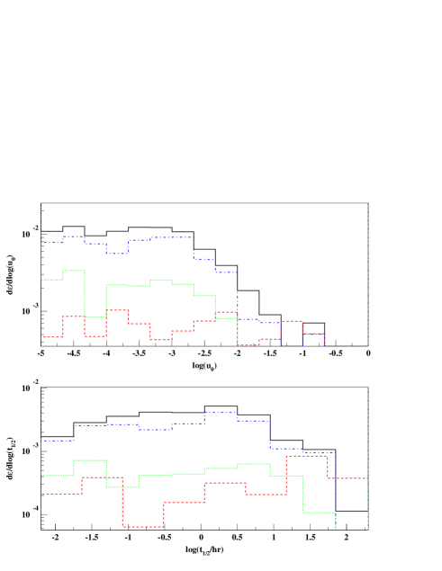
Figure 9: The detection efficiency as function of the $log(u_{0})$ (top panel) and $\log(t_{1/2}/h)$ (low panel) for two strategies of short cadence and long cadence observations. The short cadence observation with one day, two days and three days are shown with green dotted line, blue dots-dashed line and black solid line, respectively. The efficiency for the long cadence observation with the duration of one month is shown with red dashed line.

	$T_{obs}$ $(day)$	$1$	$2$	$3$	$30$
1	$N_{e}(1/day)$	4.2	13.4	18.5	0.02
2	$t_{1/2}(hr)$	16.3	20.9	22.6	62.4
3	$t_{E}(day)$	22.8	21.4	21.8	39.9

Table 3: The first three columns are for one, two and three days observation. The forth column is the result of simulation for the observation with the duration of $30$ days with the strategy of taking 30 data points during one month. All the simulation is done based on using WFC3 HST camera, except the last one with WFC2. The first row shows the number of events per one day. The second row indicates the average transit time of the events in hour and the third row indicates the average Einstein crossing time in day.

4 RESULT

In this section we report the results of the Monte-Carlo simulation as the number of events and the mean value for the parameters of the lenses. For each structure along the line of sight, we define a threshold form the simulation where a microlensing event is detected in the range of $u_{0}<u_{th}$. The overall number of events can be obtained by summing the number of events for each structure as follows:

$$\frac{N_{e}}{T_{obs}}=4\sum_{i=1}^{N_{s}}\int_{\Omega}{\tau^{i}\left<\frac{\tilde{t_{E}^{i}}}{\epsilon^{i}(\tilde{t_{E}})}\right>^{-1}{u^{i}_{th}(\theta)}^{2}\frac{dN(\theta)}{d\theta}\theta d\theta}.$$ (18)

Here, $N_{s}$ is the number of the structures, the superscript ${}^{\prime}i^{\prime}$ corresponds to the $i$th structure along the line of sight and $\epsilon^{i}(\tilde{t_{E}})$ corresponds to the detection efficiency. $<{\tilde{t_{E}^{i}}}/{\epsilon^{i}(\tilde{t_{E}})}>$ is the average value for the ratio of the reduced Einstein crossing time to the detection efficiency with the threshold impact parameter of $u_{th}$ for each structure. The integration is performed over the surface of M87 using the column density of the stars from the model. We also obtain the differential number of events ${dN}/{d\theta}$ as a function of angular separation from the center of the structure, as represented by the dashed line in Fig.4. Unlike the results from the rough estimation, the results from the Monte Carlo simulation show that the central part of the structure is better for pixel-lensing. Our simulation results in $4.2$ pixel lensing for $1$ d of observations with the HST. The corresponding parameters of the events are shown in Table 2. In order to test how sensitive the detection is to the duration of the observation, we run the Monte-Carlo simulation for the duration of $1$, $2$ and $3$ d using both with the new strategy and that of Baltz et al. (2004) for one month. We report the daily numbers of events in Table (3).

The results for the observational efficiency is shown in Fig 9, where we plot the detection efficiency in terms of $log(u_{0})$ (top panel) and $log(t_{1/2})$ (bottom panel) for two observational strategies and four observational durations. The minimum impact parameter is limited by the finite-size effect below $log(u_{0})=-2.5$, where the efficiency remains constant. The efficiency diagrams predict that intensive observations using the HST over one or a few days, with the duration of the orbital time, is much more efficient than observations over one month, taking data point per day. The new strategy increases the observational efficiency by almost one order of magnitude. Table 3 summarize the results of simulation for various observational strategies.

5 conclusion

Gould (1995) proposed an observational strategy for pixel lensing of the Virgo cluster using the HST, taking one data point per day for the duration of one month. Baltz et al. (2004) performed the observations with the WFC2 camera of the HST and found seven variable candidates, from which one was shown to be a microlensing candidate. They used one microlensing candidate and put limit on the contribution of MACHOs in the Virgo halo.

In this paper, we have proposed a new observational strategy, emphasizing the detection of the shor-duration very high magnification events. To detect such events, we need high cadence observation by HST, which means one observation per orbit for the duration of one to few days. First, we made a rough estimation of the number of observed events using this strategy. For the detailed study, we performed a Monte-Carlo simulation to obtain the number of pixel lensings events. With HST observation over $1$ d, and considering $20$ per cent of the Virgo halo to be composed of MACHOs, we expect to see $\sim 4.2$ events. If we look at the result of the observations over $2$ or $3$ d, there are more than two and three times the number of the events than for observation taken over $1$ d. We note that, with the new strategy, taking observations over 15 orbits in 1 d uses half of the observational time than one month of observations with the former observational strategy, and it increases the number of events substantially. This new strategy could provide new possibility for pixel-lensing observations on cosmological scales.

Acknowledgment We would like to thank the referee for valuable comments. We thank Mansour Karami for helping to generate the stellar population of stars and we thank Kailash Sahu for his guidance concerning the details of the HST observations.

References

- Afonso et al. (2003) Afonso, C., et al. 2003, A&A 400, L951.
- Alcock et al. (1993) Alcock, C., et al. 1993, Nature 365, L621.
- Alcock et al. (2000) Alcock, C., et al. 2000, ApJ 542, L281.
- Ansari et al. (1999) Ansari, R., et al. 1999, A&A 344, L49.
- Baillon et al. (1993) Baillon, P., Bouquet, A., Giraud-Heraud, Y. & Kaplan, J., 1993, A&A 277, L1.
- Baltz et al. (2004) Baltz E. A., Lauer, T. R., Zurek, D. R., Gondolo, P., Shara, M. M., Silk, J. & Zepf, S. E., 2004, ApJ 610, L691.
- Battaglia et al. (2005) Battaglia G., et. al. 2005, MNRAS 364, L433.
- Binney & Tremaine (1987) Binney, S., & Tremaine, S. 1987, Galactic Dynamics (Princeton, NJ: Princeton Univ. Press).
- Cignoni et al. (2006) Cignoni M., DeglInnocenti, S., PradaMoroni, P. G. & Shore, S. N. 2006, A&A 459, L783.
- Crotts (1992) Crotts A. P. S. 1992, ApJ 399, L43.
- Crotts & Tomaney (1996) Crotts A. P. S. & Tomaney A. B. 1996, ApJ 473, L87.
- Dehnen et al. (2006) Dehnen, W., Mcllaughlin, D. E. & Sachania J. 2006, MNRAS 369, L1688.
- Doherty et al. (2009) Doherty, M., et al. 2009, A&A 502, L771.
- Drive (2010) Drive S. M. 2010, Space Telescope Scince Institute, (http://www.stsci.edu/hst/wfc3)
- Einstein (1911) Einstein A. 1911, Annalen der physik, 35, L898.
- Erickcek & Law (2010) Erickcek A. L. & Law N. M., 2010, preprint(arXiv:1007.4228v1).
- Fouqué et al. (2001) Fouqué P., Solanes J. M., Sanchis T., & Balkowski C., 2001, A&A 375, L770.
- Gebhardt & Thomas (2009) Gebhardt, K. & Thomas, J. 2009, ApJ 700, L1690.
- Goerdt et al. (2007) Goerdt, T., Gnedin, O. Y., Moore, B., Diemand, J., & Stadel, J. 2007, MNRAS, 375, 191
- Gould (1995) Gould, A. 1995, ApJ 455, L44.
- Gould A. (1996) Gould, A. 1996, ApJ 470, L201.
- Hayashi et al. (1962) Hayashi. C., Hōshi, R., & Sugimoto. D. 1962, Prog. Theor. Phys. Supp., N22, L1.
- Karami (2010) Karami, M., M.Sc. thesis (2010), Sharif Univ of Technology
- Kerins et al. (2006) Kerins, E., Darnley, M. J., Duke, J. P., Gould, A., Han, C., Jeon, Y.-B., Newsam, A. & Park, B.-G. 2006, MNRAS 365, L1099.
- Kroupa et al. (1993) Kroupa, P., Tout, C.A. & Gilmore, G. 1993, MNRAS 262, L545.
- Kroupa (2001) Kroupa, P. 2001, MNRAS 322(2), L231.
- (27) Maeder A., 1973, A&A, 26, 215.
- Madrid et al. (2007) Madrid, J. P., Sparks, W. B., Ferguson, H. C., Livio, M. & Macchetto D. 2007, ApJ 654, L41.
- Marigo et al. (2008) Marigo P. et al. 2008, A&A 482, L883.
- McLaughlin (1999) McLaughlin, D. E. 1999, ApJ 512, L9.
- Mei et al. (2007) Mei, S., et al. 2007, ApJ 655, L144.
- Milsztajn & Lasserre (2001) Milsztajn, A., Lasserre, T. 2001, Nucl. Phys. Proc. Suppl 91, L413.
- Moniez (2010) Moniez, M. 2010, General Relativity and Gravitation, 42, 2047
- Navarro et al. (1996) Navarro. J. F., Frenk, C. S., & White, S. D. M. 1996, ApJ 462, L563.
- Paczyński (1986) Paczyński B., 1986 ApJ 304, L1.
- Rahvar (2004) Rahvar, S., 2004, MNRAS 347, 213.
- Romanowsky & Kochanek (2001) Romanowsky, A. J. & Kochanek, C. S. 2001, ApJ 553, L722.
- Salpeter (1995) Salpeter, E. E., 1995, ApJ 121, L161.
- Sirianni et al. (2005) Sirianni, M., et al. 2005, Astron. Soc. Pac. 117, L1049.
- Tsai (1994) Tsai, J. C. 1994, ApJ 423, L143.
- Twarog (1980) Twarog B. A. 1980, ApJ Supplement Series 44, L1.
- Weingartner & Draine (2001) Weingartner, J. C.& Draine, B. T. 2001, ApJ 548, L296.
- (43) Witt, H. J. & Mao. S. 1994, ApJ 430, L505.
- Wyrzykowski et al. (2009) Wyrzykowski, L., et al. 2009, MNRAS 397, L1228.