Dominant Multipoles in WMAP5 Mosaic Data Correlation Maps

Abstract

The method of correlation mapping on the full sphere is used to study the properties of the ILC map, as well as the dust and synchrotron background components. An anomalous correlation of the components with the ILC map in the main plane and in the poles of the ecliptic and equatorial coordinate systems was discovered. Apart from the bias, a dominant quadrupole contribution in the power spectrum of the mosaic correlation maps was found in the pixel correlation histogram. Various causes of the anomalous signal are discussed.

Key words:   cosmology: cosmic microwave background — cosmology: observations — methods: data analysis

1 INTRODUCTION

Non-Gaussian features for the low harmonics, the quadrupole and octupole, were found almost immediately after the first WMAP mission data release [1, 2, 3]. These features are expressed in the planarity and alignment of the two harmonics, which was noted by Tegmark et al. [4]. The axis along which the extrema of these multipoles are lined up in the WMAP mission map was later named the Axis of Evil [5]. Note that this axis is not the only selected axis in the mission data, the naturally selected axis lies in the Galactic plane. In the further releases of the WMAP mission data [6, 7, 8, 9] the existence of the Axis of Evil was also confirmed.

Different estimations of the significance of existence of this axis, and several hypotheses on its origin were made. Various studies, e.g. [11, 10]  investigated the contribution of background components and their influence on the alignment of multipoles ($\ell=2$ and $\ell=3$), and indicated a small probability of the background effect on the orientation of the low multipoles. In [11], where the multipole vectors were used for the estimates of this effect, it was also noted that the positions of the quadrupole and octupole axes correspond to the geometry and direction of motion of the Solar System and are perpendicular to the ecliptic plane and the plane, given by the direction to the dipole. Randomness of such an effect is estimated by the authors as unlikely at the significance level exceeding 98% and exclude the effect of residual contribution of background components. Continuing the research done, Copi et al. [12] conclude that the characteristics of low multipoles are abnormally different from random, which may be due to the statistical anisotropy of the universe at large scales, or to the problems of the ILC (Internal Linear Combination) signal deconvolution method. Park et al. [13] note that the planarity of the quadrupole and octupole is not statistically significant. They also stress that the residual photon radiation in the ILC map does not affect significantly the level of the effect.

Cosmological models were developed to explain the prominence of the axis in the orientation of multipoles. The alignment of the quadrupole and octupole could be explained within the framework of these models. Various models include the anisotropic expansion of the Universe, rotation and magnetic field [14, 15, 16].

Other studies investigated the contribution of ecliptic dust in the microwave background. Diego et al. [17] have constructed a combination of initial data of the WMAP channels: $V+W-2Q$, which was smoothed over a 7-degree diagram. The CMB is not included in this combination, however, it can be used as a tool to investigate the behavior of the large-scale residual signal. The authors have shown the presence of radiation in this residual signal. Its distribution is correlated with the position of the ecliptic plane. The paper investigates the contribution of zodiacal dust and shows that the radiation level of this contribution is not sufficient to explain the level of residual signal in the map combinations. In addition, a contribution from unresolved sources was estimated, which could also become an explanation of the observed effect. The authors do not consider this contribution sufficient as well.

Dikarev et al. [18] used the WMAP data and the infrared survey data to compute the parameters of dust particles, which could provide the corresponding contribution in the microwave background. The authors believe that the silicate beads a few millimeters in size in the zodiacal cloud and trans-Neptunian region with optical depth on the order of 10^-7 could explain additional radiation at the level of 10 $\mu$K in the microwave background in the ecliptic.

We investigated the problem of correlation properties of the WMAP maps, given the fact [19] that increased correlations were previously reported in various ILC signal distribution regions. In addition, it was proved [20, 21, 22] that a great contribution to the non-Gaussianity of data on various multipoles is given by the background components. Coming back to [19], let us note that the distribution of the correlation coefficients in mosaic areas of the map had a great shift for the correlations with the dust component of the background. This may be due to a more complex model of the dust distribution than the one currently used for the separation of components, and then the effect may occur in the correlation at other galactic latitudes.

In this paper, we continue to study the detected correlation [19] at different angular scales. To study the effect, we calculate the angular power spectrum of the mosaic correlation map and select its main harmonic components. We apply this analysis to the ILC map correlations both with the dust component, and with the synchrotron radiation.

2 MOSAIC CORRELATION METHOD

To analyze the map’s properties on different angular scales, we expand the signal distributed on the sphere into the spherical harmonics (multipoles):

$$\Delta S(\theta,\phi)=\sum_{\ell=1}^{\infty}\sum_{m=-\ell}^{m=\ell}a_{\ell m}Y_{\ell m}(\theta,\phi)\,,$$ (1)

where $\Delta S(\theta,\phi)$ are the signal variations on the sphere in polar coordinates, $\ell$ is the multipole number, $m$ is the multipole mode number. The spherical harmonics are determined as

$$Y_{\ell m}(\theta,\phi)=\sqrt{{(2\ell+1)\over 4\pi}{(\ell-m)!\over(\ell+m)!}}P_{\ell}^{m}(x)e^{im\phi},$$ (2)

where $x=\cos\theta$, and $P_{\ell}^{m}(x)$ are the associated Legendre polynomials. For a continuous function $\Delta S(x,\phi)$ the expansion coefficients $a_{\ell m}$ are expressed as

$$a_{\ell m}=\int^{1}_{-1}dx\int^{2\pi}_{0}\Delta S(x,\phi)Y^{*}_{\ell m}(x,\phi)d\phi\,,$$ (3)

where $Y^{*}_{\ell m}$ denotes a complex conjugation $Y_{\ell m}$.

The correlation properties of two maps of the signal distribution on the sphere can be described, on a given angular scale, by a correlation coefficient for the corresponding multipole $\ell$ as:

$$K(\ell)=\frac{1}{2}\frac{\sum\limits_{m=-\ell}^{l}t_{\ell m}s^{*}_{\ell m}+t^{*}_{\ell m}s_{\ell m}}{(\sum\limits_{m=-\ell}^{l}|t_{\ell m}|^{2}\sum\limits_{m=-\ell}^{\ell}|s_{\ell m}|^{2})^{1/2}}\,,$$

where $t_{\ell m}$ and $s_{\ell m}$ are the variations of two signals in a harmonic representation. The coefficient $K(\ell)$ can be used to assess the correlation between the harmonics on the sphere, i.e., to compare the properties of maps on a given angular scale. However, in the case of a search for correlated areas, which do not repeat in other regions of the sphere, this approach smears such single areas in the process of averaging over the sphere within a certain harmonic. In this case it becomes practically impossible to identify the correlated areas.

Verkhodanov et al. [19] proposed an approach, which was implemented in the second release of the GLESP package [23]. The proposed procedure makes it possible to find correlations between two maps in the areas of a certain angular size. In this method, each pixel with number $p$ subtending the solid angle $\Xi_{p}$ is assigned the cross-correlation coefficient $K(\Xi_{p}|\ell_{max})$ between the data of the two maps on the corresponding area. Thus a correlation map is constructed for two signals $T$ and $S$, where the value of each pixel $p$ ($p=1,2,...,N_{0}$, and $N_{0}$ is the total number of pixels on the sphere) with the subtending angle $\Xi_{p}$, and computed for the sphere maps with the initial resolution determined by $\ell_{max}$ is equal to

$$K(\Xi_{p}|\ell_{max})=\hskip 142.26378pt$$

$$\frac{\sum\sum\limits_{p_{ij}\in\Xi_{p}}(T(\theta_{i},\phi_{j})-\overline{T(\Xi_{p}))}(S(\theta_{i},\phi_{j})-\overline{S(\Xi_{p}))}}{\sigma_{T_{p}}\sigma_{S_{p}}}.$$ (4)

Here $T(\theta_{i},\phi_{j})$ is the value of the signal $T$ in the pixel with the coordinates $(\theta_{i},\phi_{j})$ for the initial resolution of the pixelization of the sphere; $S(\theta_{i},\phi_{j})$ is the value of the other signal in the same area; $\overline{T(\Xi_{p})}$ and $\overline{S(\Xi_{p})}$ are the mean values averaged over the area $\Xi_{p}$ and obtained from the higher resolution map data determined by $\ell_{max}$, $\sigma_{T_{p}}$, and $\sigma_{S_{p}}$ are the corresponding standard deviations in the area considered.

3 ILC AND DUST BACKGROUND COMPONENT MAP CORRELATION

In [19] we found a significant bias in the distribution of the correlation coefficients for the WMAP ILC and dust maps. Let us view this distribution in detail. To do this, we construct mosaic correlation maps with pixels having the sides of 160, 300 and 540 minutes of arc with the corresponding maximal multipoles $\ell_{max}=33$, 17 and 9 in accordance with the definition (4). The resulting maps are shown in Fig. 1.

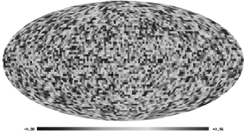
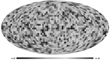
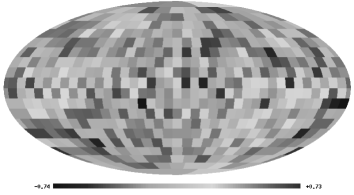
Figure 1: Maps of correlation coefficients on the sphere, constructed for mosaic correlations of the ILC and dust maps. Top to bottom: maps for the pixelization with the pixel side of 160^′, 300^′and 540^′.

Figure 2: Histograms of correlation coefficient distribution for the ILC and dust maps. Top to bottom: histograms for the pixelization with the pixel side of 160, 300 and 540^′. The dotted line, short and long dashes mark the $\pm\sigma$, $\pm 2\sigma$ and $\pm$3$\sigma$ levels in the pixel distribution for correlating random signals, computed for the $\Lambda$CDM cosmological model and dust.

Figure 3: Power spectra $C(\ell)$ of the correlation coefficient maps of the ILC signals and dust. Top to bottom: power spectra for the pixelization with the pixel side of 160, 300 and 540^′. The dotted line, short and long dashes mark the $\pm\sigma$, $\pm 2\sigma$ and $\pm$3$\sigma$ levels in the scatter of signal values for the correlation of a random map and dust.

The distribution of pixels (correlation coefficients) for the maps in Fig. 1 is demonstrated in Fig. 2. Here the $\pm\sigma$, $\pm 2\sigma$ and $\pm$3$\sigma$ levels in the pixel distribution for the correlation of a random signal and dust are marked with dotted, short and long dashed lines, respectively. These levels were computed by averaging the results of calculations for the 200 random Gaussian maps modelled in terms of the $\Lambda$CDM cosmology power spectrum. Apart from the shift in the distribution to the negative values, there is a significant distortion of the distribution shape, which distinguishes it from a normal distribution. The median values of the distributions for the correlation pixels of 160^′, 300^′  and 540^′  are equal to $-$0.2187, $-$0.2326 and $-$0.2736, respectively. It should be noted though that the resulting distribution bias is similar to the bias, obtained at the statistical evaluations of the quadrupole signal restoration quality using the ILC method  [24].

The shift of the distribution in the negative direction defines the monopole in the correlation map. It is most likely related to the procedure of component separation and is also observed in the correlations of one-dimensional cross sections [25, 26]. However, the distortion may be caused by the presence of enhanced correlations of higher multipoles in the maps. To investigate this phenomenon let us construct the angular power spectrum:

$$C(\ell)=\frac{1}{2\ell+1}\left[|a_{\ell 0}|^{2}+2\sum_{m=1}^{\ell}|a_{\ell m}|^{2}\right].$$

The power spectra of the maps with the corresponding $\ell_{max}=33$, 17 and 9 are demonstrated in Fig. 3. The dotted, short and long dashed lines here mark the $\sigma$, 2$\sigma$ and 3$\sigma$ levels in the scatter of spectrum values for the correlation of random maps and dust. The monopole signal has previously been removed. It is clear from Fig. 3 that for all the three power spectra the quadrupole is much stronger than the other harmonics. Using the expansion by the formula (1), we extract this harmonic from the correlation map data. The results are demonstrated in Fig. 4.

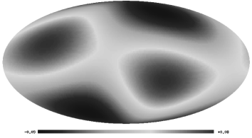
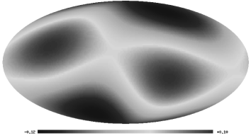
Figure 4: The quadrupole extracted from the ILC and dust correlation maps. Top to bottom: maps for the pixelization of correlations within the areas with the sides of 160, 300 and 540^′.

A peculiarity of this quadrupole is its sensitivity to both coordinate grids we selected: ecliptic and equatorial, as demonstrated in Fig. 5. The figure shows that the cold spots near the galactic poles lie in the ecliptic plane, and hot spots lie exactly in the equatorial poles.

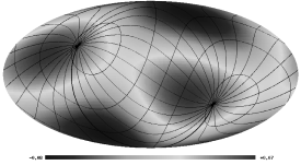
Figure 5: Ecliptic (left) and equatorial (right) coordinate grids in the quadrupole map, constructed based on the data with the pixelization of 160^′. The coordinate grid poles fall on the hot spots (light gray), and the cold spots (dark gray) lie in the equator.

Note as well the fourth harmonic in the power spectrum for these correlations with the scale of 160^′. Its amplitude is also higher than the 3$\sigma$ level. It is evident from the map of this multipole (Fig. 6) that this correlation is determined by the structures in the Galactic plane, which, in general, is anticipated on the scales of 15^∘–20^∘.

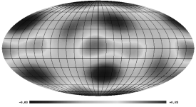
Figure 6: Map of the fourth multipole with a superimposed galactic coordinate grid. The map is calculated for the correlation window with the resolution of 160^′.

Returning to the quadrupole, we show that the removal of the Galactic plane from the calculations does not affect the position of this harmonic. For this purpose, we use the Kp0 mask, which is available from the WMAP mission website and is applied for shielding the Galactic plane and point source radiation.

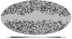
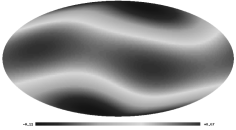
Figure 7: ILC and dust signal correlation map for the 160^′  correlation window and its statistical diagrams. The Kp0 mask is superimposed on the map. The diagrams were calculated accounting for the mask. Top left: a correlation map for the pixel side of 160^′. Top right: a histogram of pixel distribution in this map outside the Kp0 mask. The dotted, short and long dashed lines mark the $\sigma$, 2$\sigma$ and 3$\sigma$ levels in the scatter of the signal values for the correlation of a random map and dust with a superimposed mask. Bottom left: the power spectrum. Dotted and dashed lines demonstrate the scatter, estimated similarly to the previous figure. Bottom right: the quadrupole map.

Figure 7 shows the map of dust and ILC signal correlations in the areas with a side of 160^′  with a superimposed Kp0 mask. It also shows a histogram of counts outside the mask. Although a full power spectrum has no physical meaning in this case, we still use it to assess the statistical properties of the signal, applying a set of simulated maps with a superimposed mask. A statistical analysis can be then done based on the comparative characteristics. Figure 7 shows the angular power spectrum calculated on the full sphere, where the pixels located in the Kp0 mask area have the zero values inscribed. The dotted and dashed lines show the $\sigma$, 2$\sigma$ and 3$\sigma$ levels in the scatter of the signal values for the correlation of a random map and dust with a superimposed mask. Note that the ratio of the quadrupole amplitude in the spectrum in the studied correlation map to the 3$\sigma$ level is close to that anticipated from random maps, without the use of the mask it is equal to 2.2, while in the case of mask this ratio amounts to 5.5. Therefore shielding the Galactic plane increases the significance of the quadrupole harmonic contribution in the correlation map. Figure 7 as well demonstrates the quadrupole map, the axis of maxima of which is turned with respect to that shown in Fig. 4 due to the presence of the mask in the spectral analysis, and the axis of minima is unchanged.

4 CORRELATIONS BETWEEN ILC AND SYNCHROTRON BACKGROUND COMPONENT MAPS

In [19] we discussed the ILC and synchrotron radiation signal correlation maps. These maps are as well visually revealing the Galactic plane (Fig. 8), but lack a clear cut deviation of the histogram from the Gaussian distribution (Fig. 9), as it is the case of the ILC and dust emission signal distribution correlations (Fig. 2). But note that for all the three count distribution histograms, constructed for the 160, 300 and 540 ^′windows, there still exists a deviation from the Gaussian case above the 1$\sigma$ level.

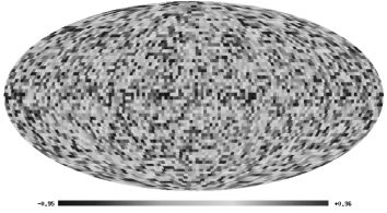
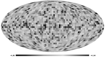
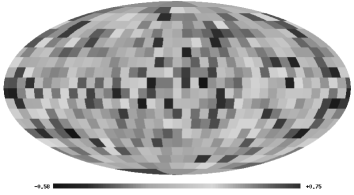
Figure 8: Maps of correlation coefficients on the sphere, constructed for mosaic correlations of the ILC and synchrotron radiation maps. Top to bottom: maps for the pixelization with the pixel side of 160^′, 300^′and 540^′.

Figure 9: Histograms of correlation coefficient distribution for the ILC and synchrotron radiation maps. Top to bottom: histograms for the pixelization with the pixel side of 160^′, 300^′and 540^′. The dotted line, short and long dashes mark the $\pm\sigma$, $\pm 2\sigma$ and $\pm$3$\sigma$ levels in the pixel distribution for correlating random signals and synchrotron radiation. The random signal is computed for the $\Lambda$CDM cosmological model.

Let us build the power spectra of the mosaic correlation maps for the ILC signal and synchrotron radiation in the same manner as we previously did for the dust maps. They are demonstrated in Fig. 10 for various correlation windows. Each figure also shows the limits of the signal scatter at the $\pm\sigma$, $\pm 2\sigma$ and $\pm$3$\sigma$ levels, calculated from the data of 200 correlation maps for the random signal in the $\Lambda$CDM cosmology. We pre-subtracted the monopole from the maps with the 160 and 300^′correlation windows.

Figure 10: Power spectra $C(\ell)$ of the correlation coefficient maps of the ILC signals and synchrotron radiation. Top to bottom: power spectra for the pixelization with the pixel side of 160^′, 300^′and 540^′. The dotted line, short and long dashes mark the $\pm\sigma$, $\pm 2\sigma$ and $\pm$3$\sigma$ levels in the scatter of signal values for the correlation of a random map and synchrotron radiation.

The spectral analysis shows that similarly to the case of dust, there is a very notable harmonic $\ell=2$. In order to study its orientation let us build its map (Fig. 11).

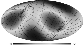
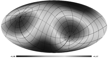
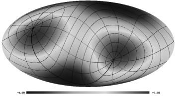
Figure 11: The quadrupole, extracted from the ILC and synchrotron radiation correlation maps. Top to bottom: maps for the pixelization of correlations within the areas with the sides of 160^′, 300^′and 540^′. The first map has the ecliptic coordinate grid superimposed, the second and the third—equatorial. The coordinate grid poles fall on the hot spots (light gray), and the cold spots (dark gray) lie in the equator.

Figure 11 draws our attention to the location of a harmonic, the orientation of which does not coincide with the Galactic plane. Although hot spots are considerably shifted relative to the maxima of the correlation maps with the dust (Fig. 4), the positions of cold spots (minima) indicate a notable sensitivity both to the ecliptic plane (Fig. 11, left, a quadrupole for the scale of 160^′), and to the equatorial plane (Fig. 11, right, a quadrupole for the scale of 540^′). Both minima in the two maps lie at the corresponding zero latitude.

5 DISCUSSION

A stable presence of the quadrupole axes linking the hot and cold spots, located in the same areas of the sky for different ILC and dust component correlation map windows in conjunction with the power spectrum, exceeding 1$\sigma$ manyfold, indicates a high level of non-Gaussianity of low multipoles in the WMAP signal. A distinctive feature of this paper from those of other authors as well demonstrating the non-Gaussianity of the WMAP low multipoles (see Introduction) is not only the method employed, but two more components: (1) we show that when cleaning the WMAP data applying the ILC technique, the dust component gives a strong anticorrelation to the emitted CMB, manifested both in the distribution of correlation coefficients, and in the angular power spectrum. The synchrotron component is considerably manifested within this approach only in the power spectrum; (2) the distribution of correlation coefficients allows speculating about a sort of a special signal that has the “knowledge” of not only the ecliptic coordinate system, but even more so about the equatorial grid.

Note that two negative spots detected in the correlation map’s quadrupole are composed of negative values, indicating the inverse behavior of the selected ILC map and background components in these areas. The negative areas of the quadrupole strictly correspond to the position of positive residual signal zones detected in [10]. This fact confirms the prominence of these WMAP map areas. An important argument from our point of view is the position of these spots, which does not seem to be entirely random. The coordinates of the minima of the quadrupole’s cold spots are close to the (0,0) and (180^∘,0) coordinates both in the ecliptic, and in the equatorial coordinate systems, and the positions of hot spots (the poles either in the ecliptic, or equatorial systems) are sensitive to the size of the selected correlation scale. We have demonstrated this effect plotting a grid on the quadrupole map (Fig. 5 and 11).

Note that we can not yet confidently tell what has caused the sensitivity to the coordinate system. We can enumerate several potential effects that may play a role in enhancing the signal in the ecliptic:

• the presence of the dust component in the ecliptic plane; despite the weakness of contribution of the zodiacal dust [10], we can not as yet rule out the effect of silicone condensates [18];

• the presence of the microwave background, determined by the solar wind; the results of research in this direction, presented in the form of signal distribution maps on the full sphere, are not yet available; in addition, such a background has to be variable owing to the solar activity;

• the residual noise associated with the inhomogeneous sensitivity of a WMAP pixel, depending on the distance from the ecliptic plane; the produced mosaic correlation and modeling for the WMAP noise map has shown very low correlation characteristics with the ILC map (Fig. 12);

  

  Figure 12: Left: pixel histogram for the mosaic correlation map of ILC and noise. Right: power spectrum of this map. The correlations were computed inside the areas with the pixel side of 160^′. The dotted line, short and long dashes mark the $\pm\sigma$, $\pm 2\sigma$ and $\pm$3$\sigma$ levels in the pixel distribution for correlating random and noise signals.

• The influence of huge dust belts of giant planets on the effects of component separation of the microwave radiation, the remnants of which are noticeable in the ecliptic plane. The giant dust ring, newly discovered by NASA’s Spitzer infrared space telescope [27], with the size larger than one degree should give an unaccounted contribution to the radiation in the ecliptic plane as a result of multiple passes through the power beam of the WMAP antenna. The level of such a contribution in the microwave range was not evaluated.

A discovery of the equatorial coordinate system in the correlations, apparent in the positions of the quadrupole hot and cold spots, remains a surprise. The possibility of its physical manifestation in the Lagrangian point L2 seems doubtful. There is no evidence of the existence of the Earth’s giant dust ring, similar to those discovered around Saturn, as it would be detectable both from Earth and from satellites. Neither do we find any signatures of a giant tail of the Earth’s magnetosphere stretching up to L2, which could host areas of microwave radiation. In this case, the effect of systematics, possibly associated with the process of observations is probable, but not clear. If we assume that non-Gaussian deviations of the low multipole characteristics can be related to the problem of the component separation, including the poorly-studied radiation of the ecliptic plane, then the question of how these correlations turn out to be sensitive to the equatorial system requires further study.

The data anticipated from the Planck mission is of much interest in this regard. These data, owing to higher resolution and sensitivity, will allow to compute and investigate mosaic correlation maps in the ecliptic and equatorial planes.

6 ACKNOWLEDGMENTS

We are grateful to P. D. Naselsky for useful discussions. We thank the NASA for making available the NASA Legacy Archive, from where we adopted the WMAP data. We are also grateful to the authors of the HEALPix [28] package, which we used to transform the WMAP maps into the coefficients $a_{\ell m}$. This work made use of the GLESP [29, 30] package for the further analysis of the CMB data on the sphere. This work was supported by the grant ”Leading Scientific Schools of Russia” and the Russian Foundation for Basic Research (grant no. 09-02-00298). O.V.V. also acknowledges partial support from the Foundation for the Support of Domestic Science (the program “Young Doctors of Science of the Russian Academy of Sciences”) and the Dynasty Foundation.

References

- [1] C. L. Bennett M. Halpern, G. Hinshaw et al., Astrophys. J. Supp. 148, 1 (2003), astro-ph/0302207.
- [2] C. L. Bennett R. S. Hill, G. Hinshaw et al., Astrophys. J. Supp. 148, 97 (2003), astro-ph/0302208.
- [3] D. N. Spergel, L. Verde, H. V. Peiris et al., Astrophys. J. Supp. 148, 175 (2003), astro-ph/0302209.
- [4] M. Tegmark, A. de Oliveira-Costa and A. Hamilton, Phys. Rev. D 68, 123523 (2003), astro-ph/03022496.
- [5] K. Land and J. Magueijo, Phys. Rev. Lett. 95 071301 (2005).
- [6] G. Hinshaw, D. N. Spergel, L. Verde et al., Astrophys. J. Supp. 170, 288 (2007), astro-ph/0603451.
- [7] D. N. Spergel et al., Astrophys. J. Supp. 170, 377 (2007), astro-ph/0603449.
- [8] G. Hinshaw, J. L. Weiland, R. S. Hill et al., Astrophys. J. Supp. 180, 225 (2009), arXiv:0803.0732.
- [9] E. Komatsu, J. Dunkley, M. R. Nolta et al., Astrophys. J. Supp. 180, 330 (2009), arXiv:0803.0547.
- [10] A. Gruppuso and C. Alessandro, JCAP 08, 004 (2009).
- [11] C. J. Copi, D. Huterer, D. J. Schwarz, and G. D. Starkman, MNRAS 367, 79 (2006).
- [12] C. J. Copi, D. Huterer, D. J. Schwarz, and G. D. Starkman, MNRAS 399, 295 (2009).
- [13] C.-G. Park, C. Park and J. R. Gott III, Astrophys. J 660, 959 (2007), astro-ph/0608129.
- [14] T. R. Jaffe, A. J. Banday, H. K. Eriksen, et al., A&A 460, 393 (2006).
- [15] M. Demianski and A. G. Doroshkevich, Phys. Rev. D 75l, 3517 (2007).
- [16] T. Koivisto and D. F. Mota, JCAP 06, 018 (2008).
- [17] J. M. Diego, M. Cruz, J. Gonzalez-Nuevo, et al., arXiv: 0901.4344 (2009).
- [18] V. Dikarev, O. Preuss, S. Solanki, et al., Astrophys. J 705, 670 (2009).
- [19] O. V. Verkhodanov, M. L. Khabibullina and E. K. Majorova, Astrophys. J. Suppl. 64, 263 (2009).
- [20] P. D. Naselsky, A. G. Doroshkevich and O. V. Verkhodanov, Astrophys. J 599, L53 (2003), astro-ph/0310542.
- [21] P. D. Naselsky, A. G. Doroshkevich and O. V. Verkhodanov, MNRAS 349, 695 (2004), astro-ph/0310601.
- [22] P. D. Naselsky and O. V. Verkhodanov, Astrophys. J. Suppl. 62, 203 (2007).
- [23] A. G. Doroshkevich, O. B. Verkhodanov, O. P. Naselsky, et al., arXiv0904.2517 (2009).
- [24] P. D. Naselsky, O. V. Verkhodanov and M. T. B. Nielsen, Astrophys. J. Suppl. 63, 216 (2008), arXiv:0707.1484.
- [25] M. L. Khabibullina, O. V. Verkhodanov, and Yu. N. Parijskij, Astrophys. J. Suppl. 63, 95 (2008).
- [26] M. L. Khabibullina, O. V. Verkhodanov, and Yu. N. Parijskij, In “Practical Cosmology”, V.II, Proc. Internat. Conf. “Problems of Practical Cosmology”, Ed. by Yu. Baryshev, Igor N. Taganov, and P. Teerikorpi (Russian Geograph. Soc., St.Petersburg, 2008), p. 239.
- [27] W. Clavin, http://www.spitzer.caltech.edu/Media/releases/ssc2009-19/release.shtml (2009).
- [28] K. Górski, E. Hivon, A. J. Banday, et al., Astrophys. J 622, 759 (2005).
- [29] A. G. Doroshkevich, P. D. Naselsky, O. V. Verkhodanov, et al., Intern. J. Mod. Phys. D 14, 275 (2003), astro-ph/0305537.
- [30] O. V. Verkhodanov, A. G. Doroshkevich, P. D. Naselsky et al., Bull. Spec. Astrophys. Obs. 58, 40 (2005).