Non-equilibrium phase transitions in biomolecular signal transduction

Abstract

We study a mechanism for reliable switching in biomolecular signal-transduction cascades. Steady bistable states are created by system-size cooperative effects in populations of proteins, in spite of the fact that the phosphorylation-state transitions of any molecule, by means of which the switch is implemented, are highly stochastic. The emergence of switching is a nonequilibrium phase transition in an energetically driven, dissipative system described by a master equation. We use operator and functional integral methods from reaction-diffusion theory to solve for the phase structure, noise spectrum, and escape trajectories and first-passage times of a class of minimal models of switches, showing how all critical properties for switch behavior can be computed within a unified framework.

I Introduction

I.1 The emergence of devices from biomolecular systems

Two related questions define a fundamental role for statistical physics in systems biology: (1). How do biomolecular systems achieve reliable “device-level” behavior when they consist of highly stochastic componentry vonNeumann:problog:56 , in particular molecular complexes held together by low-energy hydrogen or Van der Waals bonds? (2).  Are such systems structured in a modular fashion  vonDassow:SPN:00 , i.e. can complex molecular networks decompose into quasi-autonomous functional units performing identifiable tasks which are robust against many physical parameter changes and are recombinable in evolution?

The device logic of biomolecular systems employs many of the same abstractions as electronic engineering Sauro:proteomics:04 , including amplification, filtering, and switching. Switches (which use elements of amplification and filtering) are used wherever a discrete sequence of events is required, enabling committed threshold response to environmental cues during development Ferrell:xenopus:99 ; Ferrell:switch:99 , establishing “checkpoints” for intermediate states, in processes like cell division that require strict sequencing of events Tyson:CellCycle:02 , or programming the complex progressions of cell-type differentiation vonDassow:SPN:00 .

Two classes of biomolecular processes in which modular switching is widely recognized are gene expression and signal transduction. In gene expression, the switch states are associated with patterns of genes activated for protein production, and a stochastic component is introduced in the system by the small number of weakly-bound transcription factors Sasai:gene_exp:03 . In signal transduction, the states of the switch are frequently determined by the number of phosphate or methyl groups covalently attached to specific target amino acid residues on one or more dedicated proteins Goldbeter:hypersensitivity:81 . Stochasticity in this system can again be caused by the small number of proteins or the complexes these proteins form with the catalysts which promote attachment or detachment of the phosphate or methyl groups. Gene expression changes cell type on slower timescales (minutes to hours) than signal transduction (seconds), but since many cell-type changes occur in response to external signals Ferrell:xenopus:99 ; Ferrell:switch:99 , or rely on amplification and stabilization of internal signals Tyson:CellCycle:02 , switching behavior is often produced by both systems acting together.

In this paper we consider the problems of mechanism for the emergence of robust switching in stochastic molecular systems, and of quantitative estimation of the noise and stability properties of switches. We consider switching in signal transduction via the mechanism of phosphorylation (addition of phosphate groups via the action of a kinase) and dephosphorylation (removal of phosphate groups by the action of a phosphatase) since these are a common motif found in most if not all signalling networks. In addition, the relative simplicity of phosphorylation transitions lends itself to the abstraction of many real transduction cascades in terms of a few processes, allowing us to isolate the problems of formation, control, and robustness of the switch. We observe that the most fundamental unit in signal-transduction cascades is a single type of target protein with multiple phosphorylation states (called phosphoepitopes), among which transitions are naturally modeled as a reaction-diffusion process. The network properties necessary for switching, which may be distributed in real systems among several proteins in a signal-transduction cascade, or between the cascade and the genetic transcription factors for the target proteins, are readily lumped together and assigned to a single species to produce minimal models. This coarse-graining reduces network complexity while still keeping its essential regulatory features. We are able to write down exact master equations for such ideal models, and to solve them systematically with field-theoretic methods from reaction-diffusion theory.

I.2 Senses of “switching”, their uses, and how they are achieved robustly

Switching in biomolecular systems, at the least, refers to sigmoidal response to input signals, termed “ultrasensitivity” Huang:MAPK:96 . Such response implies a sharp sigmoidal but continuous response in the concentration of a molecule over a narrow range of a (stationary) signal. In contrast, bistability Tyson:Sniffers:03 is a form of switching made possible when two stable states, $S_{1}$ and $S_{2}$, co-exist over a signal range. As a consequence, bistable systems exhibit two distinct thresholds as the signal is varied, one at which a transition occurs from $S_{1}$ to $S_{2}$ and another at which the system switches back from $S_{2}$ to $S_{1}$. The separation of thresholds leads to path dependence or hysteresis, and makes a switched state more impervious to stochastic fluctuations of the signal around the transition point, than in the ultrasensitive case. Hysteresis may be obtained by adding positive feedback to sigmoidal response Ferrell:bistability:01 . Weak hysteresis may be used to stabilize input signals, equivalent to signal “debouncing” in engineering, while strong hysteresis leads to bistability, toggling, and long-term memory Lisman:bistability:85 ; Bialek:memory:01 . We will look specifically at toggling, because this subsumes all the other phenomena of interest.

The molecular mechanisms used repeatedly in signal transduction for amplification, threshold sensitivity, and switching, are shown in Fig. 1, as they are instantiated in the Mitogen-Activated Protein Kinase (MAPK) family of transduction cascades. This widely duplicated and diversified homologue family is used througout the eukaryote kingdom Kultz:stress_signals:98 , mostly to regulate gene expression in response to cell-membrane received signals. MAPK cascades employ three proteins, each with an unphosphorylated state, and respectively one, two, and two phosphorylated states. Phosphorylation and dephosphorylation of each protein is catalyzed by exogenous kinases and phosphatases, and in addition the fully-phosphorylated states of the first two proteins act as kinases (phosphorylation catalysts) on the proteins following them in the cascade. The cascade is thus an actively driven, dissipative system, maintained away from equilibrium by the supply of activated (high-energy) phosphate donors. When used for switching, MAPK cascades may have positive feedback from the output to the highest-level protein, either through gene expression or through inhibition of degradation of the active state Huang:MAPK:96 .

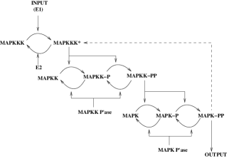
Figure 1: The catalytic topology of the mitogen-activated protein kinase (MAPK) cascades (from Ref. Huang:MAPK:96 , with dashed positive feedback arrow representing polyadenylation that inhibits degradation of the top protein). Each level in the diagram represents the phosphorylation states of a single protein, with phosphorylation and dephosphorylation transitions represented by arrows. Exogenous and internal catalysis is represented by (other) arrows pointing to the transition arrows.

The structure of MAPK and other cascades was abstracted by Goldbeter and Koshland Goldbeter:hypersensitivity:81 to the minimal system shown in Fig. 2, which they propose as the signaling counterpart to the transistor (a better analogy would be to the bistable flip-flop, as they use it). A single protein species has a single phosphorylation site. Phosphorylation and dephosphorylation occur via the action of catalysts/enzymes with which the protein can form enzyme-substrate complexes. Depending on the rate of these reactions, the steady state fractions of the phosphorylated (or unphosphorylated) protein can vary abruptly as a function of these rates. This analogy has been extended to an elaborate analysis of the properties Lisman:bistability:85 and combinatorial logic Sauro:proteomics:04 of such switches. In particular,  Lisman:bistability:85 considers the case where the the phosphorylated epitope acts as an intermolecular autocatalyst on phosphorylation transitions of any unphosphorylated proteins in the population, and shows that this leads to bistability. However, autocatalytic feedback only creates a bistable switch if the response of the underlying phosphorylation chain is sigmoidal Ferrell:bistability:01 , which in this model requires saturation of the exogenous phosphatase rate via the formation of catalyst-substrate complexes as an intermediate step between the unphosphorylated and phosphorylated states of the protein.

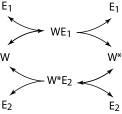
Figure 2: The Goldbeter-Koshland minimal phosphorylation couple. A single protein species has an unphosphorylated state $W$ and a singly-phosphorylated state $W^{\ast}$. Ref.Goldbeter:hypersensitivity:81 chained such couples to model intermolecular phosphorylation, in combination with exogenous catalysts that are often present for both transitions as well.

We note, however, that kinetic control through saturated complex formation is not the only way to obtain sigmoidal response, because with two or more phosphorylation sites per protein, the concentration of the fully-phosphorylated state is a sigmoidal function of the ratio of exogenous kinase to phosphatase, even when all catalysts act in the linear proportional regime (in other words, when catalyst-substrate complexes act to catalyze transitions effectively instantaneously, and are limited only by their frequency of formation through binary encounters). This occurs as long as the catalytic activity is distributive i.e., if at most one modification (phosphorylation or dephosphorylation) takes place at each enzyme-substrate encounter Gunawardena:switch:05 , and ordered (if successive phosphorylations take place at different residues, an ordered mechanism implies that dephosphorylation takes place in strictly the inverse order) Salazar:phosphate:07 .

Two of the MAPK proteins have this structure, and more significantly, the intermolecular catalysis within the cascade is nonspecific to phosphorylation reactions on a given protein, though each transition is catalyzed through an independent event Huang:MAPK:96 . We show below that, combining this form of sigmoidality with positive feedback, it is possible to obtain bistability through a non-equilibrium phase transition, in which the individual events of catalysis leads to a polarized distribution of phosphorylation states of the target protein. Such population-level cooperative effects, (proposed also in the context of genetic switches in  Sasai:gene_exp:03 ), bestow the stability of macroscopic (thermodynamic) systems on the otherwise highly stochastic events of phosphorylation and dephosphorylation. We suggest that the properties of phase-transition-mediated switching are one source of adaptive preference for multiple phosphorylation sites and non-specific catalysis, which one encounters repeatedly (histidine kinase cascades may have as many as 26 phosphorylation sites Kreegipuu:phosphobase:99 ).

Previous studies have also shown that multisite phosphorylation with saturation kinetics at each modification step can lead to bistability even in the absence of feedback Markevich:signalling:04 ; Craciun:bistability:06 . Hence both kinetic control and population-level polarization can lead robustly to bistability in some parameter domains. However, the two mechanisms are distinguished by their responses to mutations and by their control parameters. Single-molecule control causes switching properties to change if rate kinetics change, in a way that population polarization does not, while the role of nonspecific catalysis in models with population-level cooperative effects (at least in the form we will consider) creates a different kind of sensitivity. An important constraint on the evolutionary innovation, preservation, and diversification of phenotype (any expressed functionality) is the shape of its neutral network Ancel:mod_RNA:00 ; Fontana:evo_devo_RNA:02 (the degenerate space in the genotype/phenotype map with regard to that functionality). The phenotype of phase-transition-mediated switching is more nearly controlled by the topology of the catalytic network than by its kinetics, an idea that has been proposed as a source of robustness in the segment-polarity network vonDassow:SPN:00 , and theoretically grounded in the case of general enzyme-driven reaction networks in Craciun:bistability:06 .

Note that we do not study spatio-temporal correlations induced by diffusion of enzymes and/or enzyme inactivation. A recent study Takahashi:spatio-temporal:10 shows that even with the enzymes acting according to a distributive mechanism, rapid rebindings of the enzyme molecules to the substrate molecules can lead to a loss of ultrasenstivity and bistability. We do not consider the effect of protein degradation either. Our model is however a first theoretical fully stochastic study of the MAPK cascade, modelled earlier, to our knowledge, only via rate equations  Huang:MAPK:96 ; Kholodenko:negative:00 ; Markevich:signalling:04 ; Salazar:phosphate:07 ; Heinrich:mathmodels:02 or stochastic simulations Wang:stochastic:06 ; Kapuy:mol_switches:09 .

In this context, we study quantitatively the three critical properties of a phase-transition mediated switch: the conditions for existence of bistability, the noise characteristics of those fluctuations that preserve the domain in the bistable phase, and the large excursions that limit memory or reliability of the switch, and which near the threshold for bistability, can lead to finite-particle number corrections to that threshold. These have only been considered piecemeal before in other models, with conditions for bistability treated in the infinite-particle (deterministic) limit Tyson:Sniffers:03 ; Novak:CellCycle:01 , noise from internal and external sources related through ad hoc response functions Paulsson:noise:01 , and stability treated at the level of bounds on scaling, for systems already assumed reduced to one relevant dimension Bialek:memory:01 .

I.3 Reducing to appropriate models

Most biological literature on this subject focuses on phenomenological modeling of (usually mean-field behavior in) observed or designed systems vonDassow:SPN:00 ; Ferrell:xenopus:99 ; Ferrell:switch:99 ; Tyson:CellCycle:02 ; Huang:MAPK:96 ; Tyson:Sniffers:03 ; Novak:CellCycle:01 ; Markevich:signalling:04 . We are however more interested in the possibility of statistically motivated universality classification of strategies for switching, which might explain evolutionary regularities in cascades. Therefore, in addition to idealizing molecular mechanisms responsible for sigmoidal response and positive feedback as properties of single protein species, to make the polarization-based equivalent of the flip-flop from adding feedback to our Fig. 2 (equivalent to Fig. 12 of Ref. Sauro:proteomics:04 ), we advisedly exploit symmetry, of either the catalytic topology or the parameters, to make analysis tractable. This approach also aids in decomposing effects responsible for switching, and relating these to other equilibrium or non-equilibrium phase transitions. Thus our minimal models deliberately differ from the familiar cascade families in areas not directly related to the production of switching Krishnamurthy:Signaling:07 . The model of Markevich et al  Markevich:signalling:04 is also in this category in demonstrating bistability (via kinetic control) at the level of a single stage of the MAPK cascade.

The model we propose for a cooperative-phosphorylation switch is shown in Fig. 3. Each of $N$ molecules of a single type of protein has $J$ phosphorylation sites indexed $j\in 1,\ldots,J$, which we suppose for simplicity to be phosphorylated and dephosphorylated in a definite order. All phosphorylations are catalyzed by exogenous kinases, and all dephosphorylations by exogenous phosphatases. Because the enzymes are assumed to operate in the linear regime where complex formation is not rate limiting, the catalytic rate per reaction is proportional to the numbers $I$ and $P$ of kinase and phosphatase particles respectively (We set the constant of proportionality equal to one by choice of the units of time). The site modifications occur in a specific order, thus sidestepping combinatorial complexity. Furthermore, phosphorylation and dephosphorylation of substrate proteins is assumed to follow a distributive mechanism, whereby a kinase (phosphatase) enzyme dissociates from its substrate between subsequent modification events Ferrell:MAPK:97 ; Burack:nonprocessive:97 . Hence the substrate has $J+1$ states.

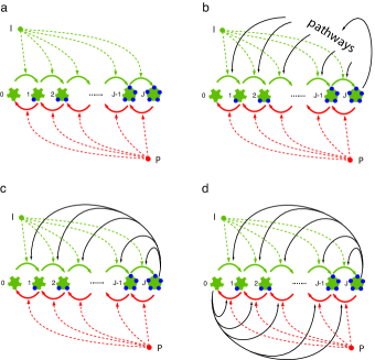
Figure 3: Multisite phosphorylation and feedback structure. (a) This panel depicts the basic phosphorylation chain without feedback in which a target protein with $J$ sites is phosphorylated by a kinase $I$ and dephosphorylated by a phosphatase $P$. The ordered succession of phosphorylations yields $J+1$ modification states, labelled $0$, $1$, $\ldots$, $J$. (b) The fully phosphorylated target protein relays a signal into pathways that eventually feed back on the phosphorylation chain. (c) Simplification of (b) in which the fully phosphorylated target protein acquires kinase activity and directly feeds back on the chain. We refer to this network configuration as the asymmetric circuit. (d) Schematic of the network with symmetric feedback in which the substrate protein is bifunctional, whereby the fully (de)phosphorylated form catalyzes (de)phosphorylation of its own precursors.

We obtain positive feedback from intermolecular autocatalysis; specifically, proteins in the $j=J$ state are kinases that act interchangeably with the exogenous kinases (unequal catalytic power between $j=J$ and exogenous kinases can easily be added, at the cost of another parameter). The phosphorylation chain with feedback is shown in the bottom half of Fig. 3. Panel (c) depicts an asymmetric topology in which the fully phosphorylated substrate catalyzes its own phosphorylation, while panel (d) shows the symmetric version in which a substrate molecule is bifunctional, acting as both a kinase and phosphatase depending on its modification state. Kinase $I$ and phosphatase $P$ are exogenous forces on the modification of the substrate, but the feedback is an endogenous force whose strength is proportional to the occupancy of the end-states of the chain. This occupancy is subject to intrinsic fluctuations and depends on the total number of substrate molecules.

The assumption of intermolecular autocatalysis is standard Lisman:bistability:85 , and we consider below the self-consistent backgrounds with kinase-only autocatalysis, as the nearest equivalent to the kinetically-controlled switch Goldbeter:hypersensitivity:81 . In order to analyse the model beyond mean-field theory (using field theoretic techniques) we go further in the interest of simplicity, and symmetrize the topology as in Fig. 3d, by making the unphosphorylated state (indexed $j=0$) a phosphatase, interchangeable with the exogenous phosphatases.

The feedback topology of the model caricatures a few elements present in biological systems. One such element is the competition between antagonistic pathways that may underlie cellular decision processes (for example Gaudet:compendium:05 ). A multisite phosphorylation chain of the type considered here could function as an evaluation point between competing and antagonistic pathways influenced by different active phosphoforms of the chain, provided these pathways feed back to the chain. In a less extreme case, the fully phosphorylated form activates another kinase which then interacts with the chain. In these scenarios, feedback is mediated by a series of intervening processes, which may well affect the propagation of fluctuations. Yet, if delays are not too large, the collapsed scheme of Fig. 3c could be a reasonable proxy with the added benefit of mathematical tractability.

A scenario corresponding more literally to our model involves a bifunctional substrate capable of both kinase and phosphatase activity, depending on the substrate’s modification state. One example is the HPr kinase/P-Ser-HPr phosphatase (HprK/P) protein, which operates in the phosphoenolpyruvate:carbohydrate phosphotransferase system of gram-positive bacteria. Upon stimulation by fructose-1,6-bisphosphate, HprK/P catalyzes the phosphorylation of HPr at a seryl residue, while inorganic phosphate stimulates the opposing activity of dephosphorylating the seryl-phosphorylated HPr (P-Ser-HPr) Kravanja:hprK:99 . Another example of a bifunctional kinase/phosphatase is the NRII (Nitrogen Regulator II) protein. It phosphorylates and dephosphorylates NRI. NRI and NRII constitute a bacterial two-component signaling system, in which NRII is the “transmitter” and NRI the “receiver” that controls gene expression. NRII autophosphorylates at a histidine residue and transfers that phosphoryl group to NRI. The phosphatase activity of NRII is stimulated by the PII signaling protein (which also inhibits the kinase activity). Several other transmitters in bacterial two-component systems seem to possess bifunctional kinase/phosphatase activity Ninfa:protein:91 .

Both the network with asymmetric topology (auto-kinase only, Fig. 3c) and the network with symmetric topology (Fig. 3d) but asymmetric catalytic concentrations $I\neq P$ undergo formally first-order phase transitions, so that regions of bistability are always metastable at finite $N$. However, in the topologically symmetric case, these continue smoothly through a second-order transition at $I=P$, in which symmetry of both topology and parameters ensures exact bistability with finite residence time in domains, at all $N$ where the phase transitions exists. This simplification permits us to estimate the residence times with an expansion in semiclassical stationary points of an effective action, without encountering the complexities of path integrals for metastable processes Coleman:AoS:85 , though numerically we expect this also to be a good approximation to residence times in metastable states with similar “barrier heights” in the first-order case. Symmetry also permits the closed-form computation of the noise kernel about the monostable phase with a unique equilibrium, which generates a natural measure for “weakness” or “strongness” of the first-order transitions at nearby values of $I/P$ as a function of $N$. We therefore perform a thorough analysis of the second-order transition, to establish methods and provide a reference solution to qualitatively understand the mechanisms of bistability and metastability in the more general cases with similar stochastic structure.

I.4 Methods of treatment for the stochastic problem

While differential equations for mean chemical concentrations (the current standard method of analysis) can give good estimates of the existence of hysteresis and bistability when approximating systems with as few as tens to hundreds of molecules, they of course preclude the treatment of noise, fluctuation-induced corrections to mean-field behavior at small particle number or near critical points, and large excursions such as domain flips (when the system switches from one bistable state to another). Pure mass-action models also ignore spatial constraints such as scaffolding by the cytoskeleton or the proteins themselves, and the dimensionality of physical diffusion in the cytosol or membranes.

A better approximation is given by the master equation for the probability of instantaneous particle distributions in models like that of Fig. 3, which in principle captures all orders of stochastic processes, though such simple models still omit spatial effects. The general properties of the master-equation (in the diffusion, or “Fokker-Planck” approximation) for a one-dimensional switch have been used to obtain scaling relations and loose bounds on the stability achievable from such a switch as a function of the number of molecules it employs Bialek:memory:01 .

Operator methods, analogous to Hamiltonian methods in quantum mechanics, have been developed in reaction-diffusion theory (see  Mattis:RDQFT:98 for a review) to efficiently handle the collective excitations that diagonalize general master equations without time-reversal symmetry. These have been used in the context of gene expression Sasai:gene_exp:03 to estimate the number of stable cell types made possible by many randomly combined transcription factors, making use of similarities to ground states of random-bond Ising models.

From the operator-valued evolution kernel, one can obtain an equivalent path-integral representation by expanding at each time in a basis of coherent states Eyink:action:96 ; Cardy:FTNEqSM:99 . Stationary-field expansion in the path integral generalizes the classical differential equation for concentrations to consistently incorporate fluctuation effects (by means of a perturbatively-corrected effective action Smith:LDP_SEA:11 ), and the sum over “approximate stationary points” of locally least-action identify the typical configuration histories associated with domain flips. More sophisticated approaches, similar to those used here, have also been used to incorporate fluctuation effects into efficient lumped-parameter expansions for networks with multiple timescales Sinitsyn:CG_chem_nets:09 .

Master equations can also be solved numerically by the Gillespie algorithm Gillespie:QTMP:94 , or simulated directly, and we use such simulations to validate our anlaytic results below. The lack of convenient symmetries in real biomolecular systems promises to make analysis intractable for most quantitative phenomenology, and recourse to numerics is likely to be the only general-purpose solution. However, the path integral’s separation of moments in a natural small-parameter expansion, and of perturbative noise from formally non-perturbative large excursions, provides an intuitive decomposition of the mechanisms fundamental to switching and stability. At mean-field approximation, we find surprising similarities of the phase transition in this driven system to the magnetization transition in the discrete, equilibrium, mean-field Ising ferromagnet, and a transition between this classical critical behavior at finite $J$ and a condensation effect more similar to Bose-Einstein condensation at $J\rightarrow\infty$. The algebraic distinction between self-consistent backgrounds, perturbative fluctuations, and non-perturbative domain flips, elementary in the analysis, is also a subtle distinction, difficult to make without systematic measurement biases, in the numerics.

I.5 Main results from the analytical treatment

The mean-field results, which are reported in detail in  Krishnamurthy:Signaling:07 , and which can also be recovered from our effective-action treatment in this paper, reproduce the standard differential equations for mass action. The stationary states arise from conditions of detailed balance between phosphorylation and dephosphorylation, self-consistent with the concentrations they produce of autocatalytic phosphoepitopes in relation to exogenous catalysts. Specifically, we show how both symmetric and asymmetric topologies create domains of mono- and bi-stability in the parameter space $\left(I/N,P/N\right)$, and how the population asymmetry in the self-consistent state depends on the coupling $g\equiv N/\sqrt{IP}$ and exogenous asymmetry $I/P$.

The perturbative expansion in Gaussian fluctuations about the self-consistent background provides a systematic construction of the noise spectrum of the phosphorylation chain. At lowest order it predicts a cusp $\sim 1/\left|g-g_{c}\right|$ in the variance of the order parameter, equivalent to the Curie-Weiss prediction for the spin-$1/2$ mean-field ferromagnet. More surprising, we find that the entire perturbative approximation to the noise spectrum on all sites is generated from a single bare mode, effectively coupled to a single Langevin field. This result replaces the ad hoc noise kernels one must entertain in the absence of a first-principles treatment Paulsson:noise:01 ; Aurell:epigenetics:02 .

The nonperturbative expansion in semiclassical configurations of locally least action predicts the leading large-$N$ dependence of the domain residence time in the bistable regime, as a function of the dimensionless rates of the problem $I/P$ and $\sqrt{IP}/N$ (though here we solve only for the symmetric case $I/P=1$, where bistability remains exact at finite particle numbers). These configurations, the dissipative equivalent to the instantons of Euclidean equilibrium field theory Coleman:AoS:85 , solve two problems. First, from the high-dimensional configuration space of the $N$-particle, $\left(J+1\right)$-site chain, they extract the one-dimensional contour of most likely configurations to mediate domain flips, assumed given in Ref. Bialek:memory:01 . Second, the action along this trajectory, $\propto N$ at fixed $\left(I/N,P/N\right)$, is the leading exponential in the residence time, for which Ref. Bialek:memory:01 correctly predicts the scaling but gives no algorithm to compute the coefficient (known in large-deviations literature as the rate function Touchette:large_dev:09 ).

Similar leading-exponential dependencies have been computed in Ref’s. Aurell:epigenetics:02 ; Roma:epigenetics:05 . For reference to this work, we note that the passage to the diffusion limit or Fokker-Planck equation in Ref. Bialek:memory:01 , and the closely-related use of the Gaussian approximation for fluctuations in Ref. Aurell:epigenetics:02 , are formally uncontrolled approximations, whose limitations and ranges of validity are pointed out in Ref. Roma:epigenetics:05 . One purpose for our paper is to present the larger systematic analysis within which such approximations arise.

I.6 Layout of the paper

Sec. II introduces the master equation for the model class of Fig. 3 c and d, and derives the phase diagram for steady states from conditions of detailed balance of the mean particle numbers. Sec. III converts the master equation, first into the equivalent representation in terms of a state in a Hilbert space, and then into the equivalent path-integral representation through an expansion in intermediate Poisson distributions. Sec. IV derives the perturbative expansion in fluctuations about the mean fields of the path integral, including the equivalent representation in terms of a Langevin equation, and the leading-order perturbative approximation to the fluctuations in the order parameter. Sec. V then considers the enlarged expansion in approximate stationary points needed to derive the trajectories and rate of domain flips. Finally, Sec. VI summarizes the consequences of these technical results for the conceptual understanding of biomolecular signal transduction and switching.

II Master equation and mean-field backgrounds

An instantaneous configuration of $N$ proteins on the $J+1$ sites of Fig. 3 defines a vector $n\equiv\left(n_{0},n_{1},\ldots,n_{J}\right)$, where $n_{j}$ is the number on site $j$. Fixed particle number implies that $n$ lives on the integer lattice in the $J$-simplex $\sum_{j=0}^{J}n_{j}\equiv N$. We denote a (generally time-dependent) probability distribution on configurations $P\!\left(n\right)$, and suppress the time index $t$ in the notation.

A stochastic process for particle hopping is completely defined by the master equation for $P\!\left(n\right)$, which is the “probability inheritance” equation induced by the transition probabilities on the simplex. For Fig. 3 with catalytic rates proportional to the number of catalytic particles, this is

$$\frac{\partial}{\partial t}P\!\left(n\right) = \sum_{j=0}^{J-1}\bigl{[}\left(I+n_{J}-{\delta}_{J,j+1}\right)\left(n_{j}+1\right)P\!\left(n+1_{j}-1_{j+1}\right)-\left(I+n_{J}\right)n_{j}P\!\left(n\right)\bigr{.}$$ (1)

$$\bigl{.}\mbox{}+\left(P+n_{0}-{\delta}_{0,j}\right)\left(n_{j+1}+1\right)P\!\left(n-1_{j}+1_{j+1}\right)-\left(P+n_{0}\right)n_{j+1}P\!\left(n\right)\bigr{]},$$

where $1_{j}$ denotes the vector with $j$th component equal to $1$ and all other components zero.

Our assumption that phosphorylation and dephosphorylation happen in a definite sequence makes transition rates from site $j$ proportional to $n_{j}$ and the catalyst concentration, without additional combinatorial factors. For the asymmetric (auto-kinase only) topology, the factors $n_{0}$ and ${\delta}_{0,j}$ in the second line of Eq. (1) are absent, and dephosphorylation depends only on the $n_{j}$ and the exogenous phosphatase number $P$.

Time-dependent average particle numbers on each site are defined as

$$\left<n_{j}\right>\equiv\sum_{n}P\!\left(n\right)n_{j},$$ (2)

and it is easy to see from Eq. (1) that $\sum_{j=0}^{J}d\left<n_{j}\right>/dt\equiv 0$.

It is also useful to write the equation for the center-of-mass of the system defined as $C\equiv\sum_{n,j}jn_{j}P(n)$. This becomes

$$\frac{\partial}{\partial t}C = N\left(I-P\right)+\left[P\left<n_{0}\right>-I\left<n_{J}\right>\right]$$ (3)

$$+ N\left[\left<n_{J}\right>-\left<n_{0}\right>\right]+\left[\left<n_{0}^{2}\right>-\left<n_{J}^{2}\right>\right]$$

As we will see later, this exact equation can be used to estimate the fluctuations of the order parameter for large $J$.

In what follows, we first look at the mean-field approximation already elaborated on in Krishnamurthy:Signaling:07 . The mean-field approximation for evolution of $\left<n_{j}\right>$ under Eq. (1) replaces all joint expectations with products of marginals: $\left<n_{j}n_{J}\right>\approx\left<n_{j}\right>\left<n_{J}\right>$, etc.

II.1 Detailed balance: symmetric topology

Under the mean-field approximation, the system of N interacting particles essentially decouples into a system of N independent particles executing a random walk on the lattice of $J+1$ sites. Within this approximation detailed balance of phosphorylation and dephosphorylation between adjacent sites in the chain holds, and depends on a catalytic ratio which we will denote $x$. For the symmetric topology, $x\equiv\left(I+\left<n_{J}\right>\right)/\left(P+\left<n_{0}\right>\right)$, and we recognize two convenient nondimensional parameters:

$$\frac{I}{P}\equiv e^{\lambda},$$ (4)

and

$$\frac{N}{\sqrt{IP}}\equiv g.$$ (5)

As autocatalysis, scaled by $N$, induces bistable order (i.e. it favours configurations in which most particles are piled up towards one or the other end of the chain), and exogenous catalysis, scaled by $I$ and $P$, induces homogeneity (configurations in which particles are uniformly spread out on the chain), $g$ is the coupling strength of the model, with strong coupling favoring broken symmetry. $I/P$ is then the measure of exogenous asymmetry.

In terms of these and the fractional occupations $\left<n_{j}\right>/N$, the catalytic ratio may be written

$$x\equiv\frac{e^{\lambda/2}+g\left<n_{J}\right>/N}{e^{-\lambda/2}+g\left<n_{0}\right>/N}\equiv e^{\xi}.$$ (6)

By induction on $j$, time-independent solutions satisfy

$$\left<n_{j}\right>=x^{j}\left<n_{0}\right>,\;0\leq j\leq J,$$ (7)

and the normalization

$$N=\sum_{j=0}^{J}\left<n_{j}\right>=\left<n_{0}\right>\frac{1-x^{J+1}}{1-x}.$$ (8)

From Eq. (6) and Eq. (7) we can evaluate

$$\frac{g}{N}\left<n_{J}-n_{0}\right>=\frac{2\sinh\left(\frac{\xi-\lambda}{2}\right)\sinh\left(\frac{J}{2}\xi\right)}{\sinh\left(\frac{J-1}{2}\xi\right)},$$ (9)

and we can rewrite Eq. (8) as

$$\frac{\left<n_{J}-n_{0}\right>}{N}=\frac{2\sinh\left(\frac{\xi}{2}\right)\sinh\left(\frac{J}{2}\xi\right)}{\sinh\left(\frac{J+1}{2}\xi\right)}.$$ (10)

When Eq. (9) and Eq. (10) are nonzero, they have the ratio

$$g=\frac{\sinh\left(\frac{\xi-\lambda}{2}\right)\sinh\left(\frac{J+1}{2}\xi\right)}{\sinh\left(\frac{\xi}{2}\right)\sinh\left(\frac{J-1}{2}\xi\right)}.$$ (11)

For $I\neq P$, Eq. (11) always holds (though it may be negative or singular), while for $I=P$ we have the possibility of the degenerate case where $\left<n_{J}-n_{0}\right>=0$ and $g$ is unconstrained. For $g<g_{C}\!\left(\lambda=0\right)$ (a second-order critical point) this is the stable asymptotic distribution, while for $g>g_{C}\!\left(\lambda=0\right)$ it is unstable. The graph of $g$ versus $\xi$ for a few (non-positive) values of $\lambda$ at $J=2$ is shown in Fig. 4. (Positive $\lambda$ generate curves reflected through $\xi=0$.) The graph defines a pseudo-inverse $\xi\!\left(g\right)$, which gives the stationary solutions within the mean-field approxiation. Where $\xi$ is triple-valued (not a well-defined inverse), the central branch is in all cases unstable, and the two outer branches are stable.

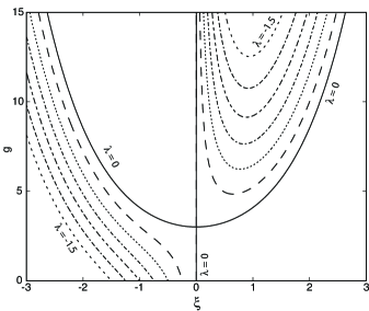
Figure 4: $g\!\left(\xi\right)$ from Eq. (11) along contours of constant $\lambda$, for which the two branches proceed outward from the $\xi=0$ line in order of increasing $\left|\lambda\right|$ (different $\lambda$ values are depicted by different line styles). The branches with the lowest and largest values of $\lambda$ are marked on the figure. The other $\lambda$ values can be read on the left from the intersection with the abscissa where $\xi=\lambda$. Where $g\!\left(\xi\right)$ has a single-valued inverse, that function $\xi\!\left(g\right)$ defines the unique steady-state distributions. Where the inverse is triple-valued, the largest $\left|\xi\right|$ are stable solutions, and the central branch is unstable.

The character of the curves in Fig. 4 is preserved for all $J>2$, though the derivative of the stable curve for $I=P$ above its critical point becomes discontinuous at $\xi=0$ for $J\rightarrow\infty$. This discontinuity is related to the transition from Curie-Weiss to Bose-Einstein-like behavior of the order parameter, discussed below. The curves corresponding to all $\lambda$ have regular limits at large $J$.

We can identify a set of $g_{C}\!\left(\lambda\right)$ as the local minima in Fig. 4 above which the $\xi\!\left(g\right)$ graph becomes triple-valued. The $\lambda\rightarrow 0$ limit of these minima smoothly converges on the second-order critical coupling

$$g_{C}\!\left(\lambda=0\right)\equiv\frac{J+1}{J-1}.$$ (12)

Converting the pair $\bigl{(}\lambda,g_{C}\!\left(\lambda\right)\bigr{)}$ to $\left(I/N,P/N\right)$ values yields the phase diagram shown in Fig. 5 for a range of $J$ values. The interior region $I\sim P$ and sufficiently small $\sqrt{IP}/N\equiv 1/g$ is bistable, and outside this region the sign of $\xi=\log x$ equals that of $\lambda\equiv\log I/P$. As we demonstrate in Krishnamurthy:Signaling:07 , these theoretical estimates match very well with data from Monte carlo simulations.

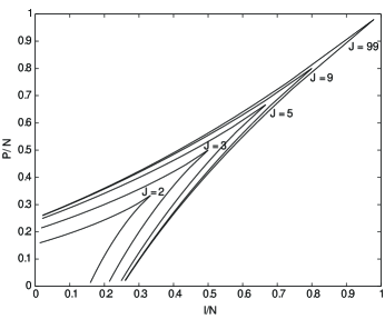
Figure 5: Phase diagram for the symmetric topology, from the minima $g_{C}\!\left(\lambda\right)$ of Fig. 4, and their equivalents for a range of $J$. The regions inside the chevrons are bistable.

II.2 Detailed balance: asymmetric topology

In the auto-kinase-only asymmetric model, positive $\lambda$ ($I>P$) is never bistable, because the particles are already biased toward $n_{J}$, the only site with positive feedback. Therefore we graph only $\lambda\leq 0$, though the algebraic solutions are valid everywhere.

Instead of Eq. (6), the catalytic ratio is $x\equiv\left(I+\left<n_{J}\right>\right)/P$, which reduces in nondimensional parameters to

$$x\equiv\frac{e^{\lambda/2}+g\left<n_{J}\right>/N}{e^{-\lambda/2}}\equiv e^{\xi}.$$ (13)

Equations (7) and (8) still hold, but instead of Eq. (9) we choose the reduction

$$g\frac{\left<n_{0}\right>}{N}=\frac{2\sinh\left(\frac{\xi-\lambda}{2}\right)}{\exp\left[\left(J-\frac{1}{2}\right)\xi\right]}.$$ (14)

The appropriate reduction of Eq. (8), counterpart to Eq. (10), is now

$$\frac{\left<n_{0}\right>}{N}=\frac{\sinh\left(\frac{\xi}{2}\right)}{\exp\left(\frac{J}{2}\xi\right)\sinh\left(\frac{J+1}{2}\xi\right)}.$$ (15)

Eq. (14) and Eq. (15) are regular at all $\xi$, so we always have a defined function $g\!\left(\xi\right)$, of the form

$$g=\frac{2\sinh\left(\frac{\xi-\lambda}{2}\right)\sinh\left(\frac{J+1}{2}\xi\right)}{\sinh\left(\frac{\xi}{2}\right)\exp\left(\frac{J-1}{2}\xi\right)}.$$ (16)

A graph at $J=2$, which is the asymmetric-topology counterpart to Fig. 4, is shown in Fig. 6. In the bistable phase, there are still three branches for $\xi$ at given $g$, with the outer two stable and the central one unstable. The obvious differences are that now there is a maximal $\lambda$ for bistability, and that the leftmost stable branch at any $\lambda$ moves positively in $\xi$ as $g$ increases because of the asymmetric topology, whereas in the symmetric topology it moved negatively in $\xi$.

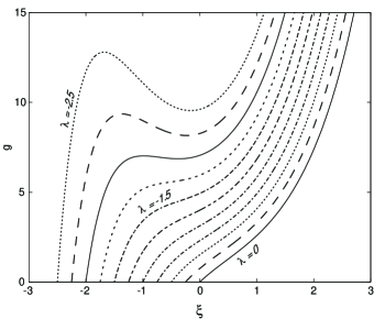
Figure 6: $g\!\left(\xi\right)$ along contours of constant $\lambda$ for the asymmetric topology, $J=2$ and the same $\lambda$ values as in Fig. 4. The maximal $\lambda$ for bistability generates the curve whose minimum derivative is zero.

At any $\lambda$ below a (negative) $J$-dependent threshold, we can extract the minimal and maximal $g$ values for bistability (below the minimum, $\xi$ follows $\lambda\equiv\log\left(I/P\right)$ qualitatively; above the maximum, only the largest-$\xi$ branch is stable because of too-strong positive feedback). Inverting $g_{\mbox{\scriptsize min}}\!\left(\lambda\right)$ and $g_{\mbox{\scriptsize max}}\!\left(\lambda\right)$ to $\left(I/N,P/N\right)$, we obtain the phase diagram for bistability shown in Fig. 7.

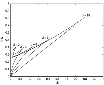
Figure 7: The phase diagram for auto-kinase feedback only. The domains of bistability are somewhat smaller than in Fig. 5, and are shifted toward smaller $I/P$, but otherwise the characteristics are qualitatively and even quantitatively similar.

The upper boundary of each bistable region, defined by $g_{\mbox{\scriptsize min}}\!\left(\lambda\right)$, is a distorted counterpart to the upper $g_{C}\!\left(\lambda\right)$ branch in Fig. 5, and the two converge to the same limit as $J\rightarrow\infty$ (where feedback from $n_{0}$ becomes irrelevant). The lower boundary, defined by $g_{\mbox{\scriptsize max}}\!\left(\lambda\right)$, replaces the reflected lower $g_{C}\!\left(\lambda\right)$ branch in Fig. 5, and converges to the diagonal $I=P$ at $J\rightarrow\infty$.

Thus we see that classically, the first-order phase transitions are similar for symmetric and asymmetric feedback topology, one being deformable into the other in the $\left(I/N,P/N\right)$ parameter space. (We could have performed this continuation smoothly by weighing the $n_{0}$ catalytic strength with a parameter $\varepsilon\in\left[0,1\right]$.) Further, the first-order transition in $g$ along any $I/P$ ray in the symmetric topology continues smoothly through the second-order transition at $I/P=1$, at the apex of the domain of bistability. Whether the first-order transitions in the neigborhood of $I/P=1$ are strong or weak depends on the $\xi$-support of the stationary solution for $P\!\left(n\right)$ (a function of $N$), in relation to the difference between the stable mean values at $g_{C}\!\left(\lambda\right)$.

II.3 Phase transition and order parameter versus $J$

We now restrict attention to the case of symmetric topology and exogenous catalysis setting $I=P\equiv q$, and consider the behavior of the natural mean-field order parameter $\left|\left<n_{J}-n_{0}\right>\right|/N$ as a function of $J$. Expanding Eq. (10) in small $\xi$, and inverting Eq. (11) relative to $g_{c}\equiv g_{C}\!\left(\lambda=0\right)$ in Eq. (12), we find the mean-field critical scaling of the discrete Ising ferromagnet, up to a $J$-dependent prefactor:

$$\frac{\left|\left<n_{J}-n_{0}\right>\right|}{N}\approx\frac{\sqrt{6J}}{J+1}{\left(\frac{g}{g_{c}}-1\right)}^{1/2}.$$ (17)

The small-$\xi$ approximation is valid for $g-g_{c}\lesssim g_{c}-1$, above which the order parameter saturates to a $J$-independent envelope value

$$\frac{\left|\left<n_{J}-n_{0}\right>\right|}{N}\rightarrow 1-\frac{1}{g}.$$ (18)

The exact mean-field prediction for $\left|\left<n_{J}-n_{0}\right>\right|/N$ versus $g$ from Equations (10) and (11) is compared to numerical simulations for $J+1=\left[5,10,100\right]$, in Fig. 8.

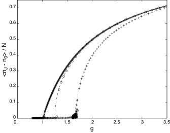
Figure 8: Order parameter $\left|\left<n_{J}-n_{0}\right>\right|/N$ for the symmetric phosphorylation chain: mean-field theory (lines) and simulations (symbols). $J+1=\left[5,10,100\right]$ corresponds to $\left[\mbox{dot},\mbox{dash},\mbox{solid}\right]$ for lines and $\left[\mbox{+},\mbox{o},\mbox{$\times$}\right]$ for symbols. Particle numbers used in the simulations are respectively $N=[4000,2000,400]$.

Since $g_{c}-1\rightarrow 2/J$ for large $J$, Eq. (18) also gives the behavior in the formal $J\rightarrow\infty$ limit. The derivative of the order parameter converges to one in arbitrarily small neighborhoods of the critical point, rather than to $\infty$ as in the Curie-Weiss regime; thus $J\rightarrow\infty$ defines a different universality class than any finite $J$. Qualitatively, the distinction between small and large-$J$ is determined by whether one or both reflecting boundaries are sensed by the near-critical symmetry-broken state. The large-$J$ transition resembles Bose-Einstein condensation in the sense that either $n_{0}$ or $n_{J}$ accounts for a finite fraction of the particles, with the remainder “thermalized” with an exponential distribution in $j$ into the interior, at “temperature” self-consistently determined by $q/N=1/g$. To understand the nature of these transitions beyond mean-field theory we introduce the operator and path-integral representations of the master equation and its solutions.

III Operator, state, and path integral representations

III.1 Operators, states, and time evolution

The operator representation of master equations from reaction-diffusion theory Mattis:RDQFT:98 ; Cardy:FTNEqSM:99 begins by introducing raising and lowering operators ${a}_{j}^{\dagger}$, $a_{j}$ for each site on the lattice, with the commutation relations of orthogonal quantum harmonic oscillators $\left[a_{j},{a}_{j^{{}^{\prime}}}^{\dagger}\right]\equiv{\delta}_{j,j^{{}^{\prime}}}$. These define a Hilbert space through their action on a “vacuum” state ${a}_{j}\left|0\right)\equiv 0,\forall j$, and its conjugate $\left(0\right|{a}_{j}^{\dagger}\equiv 0,\forall j$.

Number states indexed by the vector $n$ are defined through the action of the raising operators

$$\left|n\right)\equiv\prod_{j=0}^{J}{\left({a}_{j}^{\dagger}\right)}^{n_{j}}\left|0\right),$$ (19)

and differ from quantum-mechanical number states in being normalized with respect to a universal Glauber state Mattis:RDQFT:98 ; Cardy:FTNEqSM:99

$$\left(0\right|e^{\sum_{j}a_{j}}\left|n\right)=1,\forall n.$$ (20)

The number operator for each $j$ is defined as ${\hat{n}}_{j}\equiv{a}_{j}^{\dagger}{a}_{j}$, and extracts the appropriate coefficient from $n$ in the Glauber norm,

$$\left(0\right|\exp\left(\sum_{j^{\prime}}a_{j^{\prime}}\right){\hat{n}}_{j}\left|n\right)=n_{j}.$$ (21)

A classical distribution $P\!\left(n\right)$ has the state representation in the $n$ basis

$$\left|\psi\right)\equiv\sum_{n}P\left(n\right)\left|n\right).$$ (22)

$\left|\psi\right)$ is equivalent to a generating function $f\!\left(z\right)$ of a $\left(J+1\right)$-component complex vector $z$, under the association ${a}_{j}^{\dagger}\leftrightarrow z_{j}$, ${a}_{j}\leftrightarrow\partial/\partial z_{j}$. Glauber normalization is equivalent to a prescription for shifting $z_{j}\rightarrow z_{j}+1$, and evaluating the resulting function at $z_{j}=0,\forall j$. A thorough treatment of these methods for handling generating functions and functionals is provided in Ref. Smith:evo_games:11 in the context of the analysis of master equations for evolutionary games. However for the treatment that follows below, we need only the definitions provided above in order to proceed.

The master equation (1) corresponds to state evolution equation known as the Liouville equation

$$\frac{d}{dt}\left|\psi\right)=-\Omega\left|\psi\right),$$ (23)

in which the nonlinear, diffusive Liouville operator that evolves the state in time is given by

$$\Omega=q\sum_{j=0}^{J-1}\left({a}_{j+1}^{\dagger}-{a}_{j}^{\dagger}\right)\left[\left(1+\frac{{\hat{n}}_{0}}{q}\right){a}_{j+1}-\left(1+\frac{{\hat{n}}_{J}}{q}\right){a}_{j}\right]$$ (24)

Here $I=P\equiv q$ as mentioned earlier. The differential equation (23) is formally reduced to quadrature to give the time-dependent state relation

$$\left|{\psi}_{t}\right)\equiv e^{-\Omega t}\left|{\psi}_{0}\right).$$ (25)

Normalization of $P\!\left(n\right)$ and the number states $\left|n\right)$ implies $\left(0\right|\exp\left(\sum_{j}a_{j}\right)\left|{\psi}_{t}\right)=1,\forall t$. We further recognize the exogenous catalytic strength $q\equiv 1/\tau$ as defining a natural timescale, and the natural coupling $g\equiv N/q$ in Eq. (24), as before.

III.2 Coherent-state expansion and path integral

At weak nonlinearity (small $g$), it is both intuitive and computationally efficient to expand solutions to Eq. (25) in eigenvectors of the annihilation operators $a_{j}$ Cardy:FTNEqSM:99 , which are the Poisson distributions in $n_{j}$. We start with a normalized initial state arbitrarily parametrized by mean occupation numbers

$$\left|{\psi}_{0}\right)=\exp\left(\sum_{j}{\bar{n}}_{j}\left(a_{j}^{\dagger}-1\right)\right)\left|0\right),$$ (26)

in which judicious choice of the ${\bar{n}}_{j}$ cancels surface terms associated with transients. (Self-consistency of these parameters with stationarity under $\Omega$ may be used from the operator representation to obtain moments of $P\!\left(n\right)$, as was done in Ref. Sasai:gene_exp:03 , though we will proceed directly to the time-dependent field action here.) To form a basis for coherent-state expansion (again, see Cardy:FTNEqSM:99 for detials of this procedure) at increments of time, we introduce a complex-valued vector field ${\phi}_{t}\equiv{\left({\phi}_{0},{\phi}_{1},\ldots,{\phi}_{J}\right)}_{t}^{T}$, and its adjoint ${\phi}^{\dagger}_{t}$. At a set of $t^{{}^{\prime}}=k\Delta t$, we insert the representation of identity

$$\int\frac{d{\phi}^{\dagger}_{t^{{}^{\prime}}}\,d{\phi}_{t^{{}^{\prime}}}}{\pi}e^{-{\phi}^{\dagger}_{t^{{}^{\prime}}}\cdot{\phi}_{t^{{}^{\prime}}}}e^{a^{\dagger}\cdot{\phi}_{t^{{}^{\prime}}}}\left|0\right)\left(0\right|e^{{\phi}^{\dagger}_{t^{{}^{\prime}}}\cdot a}=\sum_{n}\left|n\right)\left(n\right|=I$$ (27)

into $\left(0\right|\exp\left(\sum_{j}a_{j}\right)\left|{\psi}_{t}\right)$, expressed through Eq. (25) and Eq. (26) as $\left(0\right|\exp\left(\sum_{j}a_{j}\right)e^{-\Omega t}\exp\left(\sum_{j}{\bar{n}}_{j}\left(a_{j}^{\dagger}-1\right)\right)\left|0\right)$. Though the coherent states are overcomplete, phase cancellations in Eq. (27) leave the proper complete number basis at each $t^{{}^{\prime}}$.

By now-standard procedures Mattis:RDQFT:98 ; Cardy:FTNEqSM:99 we recognize that the fields $\phi$ and ${\phi}^{\dagger}$ have somewhat different roles, with fluctuations in $\phi$ about its mean value corresponding roughly to fluctuations in number, and those in ${\phi}^{\dagger}$ sampling moments of the generating functional $\left|\psi\right)$. Thus we expand the complex-conjugate coefficients ${\phi}^{*}_{j}$ of the (row) vector ${\phi}^{\dagger}$ at each time as ${\phi}^{*}_{j}\equiv{\tilde{\phi}}_{j}+1$ at each $t$, with shorthand ${\phi}^{\dagger}_{t}\equiv{\tilde{\phi}}_{t}+1$, leaving $\phi$ to be determined physically. The resulting normalized generating functional has the path-integral representation

$$\left(0\right|\exp\left(\sum_{j}a_{j}\right)\left|{\psi}_{t}\right)=\int{\cal D}{\tilde{\phi}}\,{\cal D}\phi e^{-\int dtL}e^{{\tilde{\phi}}_{0}\cdot\left(\bar{n}-{\phi}_{0}\right)},$$ (28)

in which the diffusive “Lagrangian” is

$$L\left({\tilde{\phi}},\phi\right)={\tilde{\phi}}\cdot\frac{\partial\phi}{\partial t}+\Omega\left({\tilde{\phi}}+1,\phi\right).$$ (29)

The Liouville operator (24) has induced a complex-valued function of fields $\Omega\left({\tilde{\phi}}+1,\phi\right)$ through the substitution ${a}_{j}^{\dagger}\rightarrow{\tilde{\phi}}_{j}+1$, $a_{j}\rightarrow{\phi}_{j}$. We will see that, up to care with signs and contours of integration that depend on what we wish to extract from this function, it behaves as the equivalent of a Hamiltonian for an equilibrium system, with a few structural differences characteristic of stochastic processes(elaborated also in  Smith:evo_games:11 ). The measure ${\cal D}{\tilde{\phi}}\,{\cal D}\phi$ in Eq. (28) is defined formally by the skeletonization procedure for insertion of the coherent states, but in practice is usually defined implicitly by perturbation theory in the diffusive Green’s function.

Linearization of $\Omega$ in either Eq. (23) or Eq. (28) (i.e. keeping only terms linear in ${\tilde{\phi}}$) provides the natural expansion in independent collective fluctuations of the master equation and gives results for expectation values which are identical with the mean-field results presented earlier. In the field form (29) it further provides a convenient and intuitive background-field expansion, in which the backgrounds represent locally best-fit Poisson distributions with mean number equal to ${\phi}^{\ast}_{j}{\phi}_{j}$ for each component $j$.

III.3 Structure of reaction-diffusion Lagrangians

To make use of the form of $\Omega$, we introduce two projection matrices onto the catalytic sites $j=0,J$, $P_{\pm}$ with components ${\left(P_{+}\right)}_{jj^{{}^{\prime}}}\equiv{\delta}_{j,J}{\delta}_{j^{{}^{\prime}},J}$, and ${\left(P_{-}\right)}_{jj^{{}^{\prime}}}\equiv{\delta}_{j,0}{\delta}_{j^{{}^{\prime}},0}$, and linear-diffusion matrices

$$D_{+}\equiv\left[\begin{array}[]{rrrrr}1&\mbox{ }&&&\\ -1&&\ddots&&\\ &&\ddots&1&\\ &&&-1&0\end{array}\right],$$ (30)

$$D_{-}\equiv\left[\begin{array}[]{rrrrr}0&-1&\mbox{ }&&\\ &1&&\ddots&\\ &&&\ddots&-1\\ &&&&1\end{array}\right],$$ (31)

corresponding to phosphorylation and dephosphorylation transitions, respectively.

Noting that for $1^{T}$ the row vector of all ones, $1^{T}D_{\pm}\equiv 0$, we can use ${\phi}^{\dagger}$ or ${\tilde{\phi}}$ as it is convenient, to write

$$\frac{1}{q}\Omega\left({\phi}^{\dagger},\phi\right) = \left(1+\frac{1}{q}{\phi}^{\dagger}P_{-}\phi\right){\phi}^{\dagger}D_{-}\phi$$ (32)

$$\mbox{}+\left(1+\frac{1}{q}{\phi}^{\dagger}P_{+}\phi\right){\phi}^{\dagger}D_{+}\phi.$$

We extract the overall $N$-dependence of the action in the path integral by descaling time with the definition $dz\equiv dtq\equiv dt/\tau$, and rescaling the Lagrangian to a Lagrangian density per particle, to write

$$e^{-\int dtL}=e^{-N\int dz\hat{L}},$$ (33)

with $\hat{L}\equiv L/qN$. If we similarly descale the field $\phi\rightarrow\hat{\phi}\equiv\phi/N$, and the Liouvillian $\Omega\rightarrow\hat{\Omega}\equiv\Omega/qN$, we have the Lagrangian density in terms of the natural coupling $g=N/q$:

$$\hat{L}={\tilde{\phi}}\,{\partial}_{z}\hat{\phi}+\hat{\Omega}\left({\phi}^{\dagger},\hat{\phi}\right),$$ (34)

where

$$\hat{\Omega}\left({\phi}^{\dagger},\hat{\phi}\right) = \left(1+g{\phi}^{\dagger}P_{-}\hat{\phi}\right){\phi}^{\dagger}D_{-}\hat{\phi}$$ (35)

$$\mbox{}+\left(1+g{\phi}^{\dagger}P_{+}\hat{\phi}\right){\phi}^{\dagger}D_{+}\hat{\phi}.$$

Note that the natural fields define the relative number operator ${\phi}^{\dagger}_{j}{\hat{\phi}}_{j}=n_{j}/N\equiv{\nu}_{j}$, satisfying $\left<\sum_{j=0}^{J}{\nu}_{j}\right>\equiv 1$. Now not only are the fields ${\phi}^{\dagger}$ and $\hat{\phi}$ expanded about different backgrounds, comparable fluctuations of $\tilde{\phi}$ and $\hat{\phi}$ correspond to fluctuations of ${\phi}^{\dagger}$ and $\phi$ on scales differing by $N$, with large $N$ defining the domain of perturbation theory.

To expand the functional integral (28) in Gaussian fluctuations, we further separate out mean values from the fields, introducing notation $\tilde{\phi}\equiv\bar{\tilde{\phi}}+\varphi$ (so putting $\bar{{\phi}^{\dagger}}=\bar{\tilde{\phi}}+1^{T}$ and ${\phi}^{\dagger}=\bar{{\phi}^{\dagger}}+\varphi$). Using a compact notation ${\hat{\Omega}}^{i}_{j}$ for the tensor of $i$ ${\phi}^{\dagger}$-derivatives and $j$ $\hat{\phi}$-derivatives of ${\hat{\Omega}}$, the second-order Taylor expansion in $\varphi$ is exact:

$$\hat{L} = \bar{\tilde{\phi}}\cdot{\partial}_{z}\hat{\phi}+\hat{\Omega}\left(\bar{{\phi}^{\dagger}},\hat{\phi}\right)$$

$$\mbox{}+\varphi\cdot\left[{\partial}_{z}\hat{\phi}+{\hat{\Omega}}^{1}\left(\bar{{\phi}^{\dagger}},\hat{\phi}\right)\right]+\frac{1}{2}{\varphi}^{2}:{\hat{\Omega}}^{2}\left(\hat{\phi}\right),$$

and ${\hat{\Omega}}^{2}$ is independent of $\bar{{\phi}^{\dagger}}$.

The background $\bar{\tilde{\phi}}\equiv 0$ makes the first line of Eq. (LABEL:eq:L_varphi_expand) vanish for general $\hat{\phi}$, and for more general $\bar{\tilde{\phi}}$ we can expand $\hat{\phi}$ in a classical background and perturbations, in which the linear order vanishes at that $\bar{\tilde{\phi}}$. The $\varphi$-linear term in the second line of Eq. (LABEL:eq:L_varphi_expand) enforces a $\delta$-functional if $\varphi$ is rotated to an imaginary integration contour, and negative eigenvalues of ${\hat{\Omega}}^{2}\left(\hat{\phi}\right)$ only soften the $\delta$-functional for their corresponding $\varphi$ eigenvectors with a convergent Gaussian envelope. We handle these eigenvalues in perturbation theory with a Hubbard-Stratonovich transformation Weinberg:QTF_II:96 and a Langevin (auxiliary) field  Cardy:FTNEqSM:99 . We see below that in phases with no symmetry breaking, the eigenvalues of ${\hat{\Omega}}^{2}\left(\hat{\phi}\right)$ are all zero or negative.

Positive eigenvalues of ${\hat{\Omega}}^{2}\left(\hat{\phi}\right)$, of which one appears in the phase of symmetry breaking in this problem, require different treatment. They produce a divergent envelope for the $\delta$-functional integral if $\varphi$ is integrated along an imaginary contour, while a real contour for a $\varphi$ eigenvector does not enforce the expected $\delta$-functional for the corresponding component of the diffusion equation. We expect, from experience with Euclidean field theories for reversible systems, that these eigenvectors signal the existence of a continuous class of “approximate” stationary points generally termed instantons Coleman:AoS:85 . $\varphi$ diverges initially along a real contour, but for the appropriate joint background of $\hat{\phi}$, nonlinearities in the equations of motion extend the divergence into a bounded trajectory of locally least $\int dz\hat{L}$, representing domain flips (a fluctuation that takes the system from one of the bistable phases to the other) in the symmetry-broken phase. The integration over the unstable fluctuations of $\varphi$ are not handled in Gaussian perturbation theory about the static background, but replaced (with a proper measure term) with the integral over all time-translates of the approximate stationary solutions.

III.4 Symmetries and conservations

Foregoing formal treatment of the convergence of Langevin perturbation theory and its regulation by approximate stationary points Cardy:Instantons:78 , we observe two important global symmetries of the theory which hold as field identities and also order-by-order in a large-$N$ expansion. These are useful in numerically solving for approximate stationary points in low-dimensional examples.

The classical equations of motion following from Eq. (LABEL:eq:L_varphi_expand) and its equivalent expansion for $\hat{\phi}=\bar{\hat{\phi}}+{\hat{\phi}}^{{}^{\prime}}$ are

$${\partial}_{z}\bar{\hat{\phi}}+{\hat{\Omega}}^{1}\left(\bar{{\phi}^{\dagger}},\bar{\hat{\phi}}\right)=0,$$ (37)

$$-{\partial}_{z}\bar{{\phi}^{\dagger}}+{\hat{\Omega}}_{1}\left(\bar{{\phi}^{\dagger}},\bar{\hat{\phi}}\right)=0.$$ (38)

Both are ${\cal O}\!\left(N^{0}\right)$, as $\hat{L}$ is defined in terms only of $z$, $g$, and descaled fields. The equivalent equations in terms of ${\phi}^{\dagger}$ and $\phi$, resulting from shifts of the fields in the measure, generate Ward identities of the theory to all orders in $N$.

The transformation ${\phi}^{\dagger}\rightarrow e^{\Lambda}{\phi}^{\dagger}$, $\hat{\phi}\rightarrow e^{-\Lambda}\hat{\phi}$ at constant $\Lambda$ is a symmetry of $\hat{L}$ at general ${\phi}^{\dagger},\hat{\phi}$, whose associated Noether charge is number: ${\partial}_{z}\left({\phi}^{\dagger}\cdot\hat{\phi}\right)=0$ as a field equation. Time-translation is also a symmetry of $\hat{L}$ whose Noether charge is the potential: ${\partial}_{z}\left(\hat{\Omega}\right)=0$. Both of these follow immediately as properties of the classical solutions of Eq’s. (37) and (38). About backgrounds that are, or converge to, $\bar{\tilde{\phi}}\equiv 0$, the constraints $\bar{{\phi}^{\dagger}}\cdot\bar{\hat{\phi}}=1$ and ${\hat{\Omega}}\left(\bar{{\phi}^{\dagger}},\bar{\hat{\phi}}\right)=0$ specify a $2J$-dimensional subspace of field configurations in which all classical trajectories must lie.

We further note that, due to the quartic form (35),

$$\bar{\tilde{\phi}}\cdot{\partial}_{z}\bar{\hat{\phi}} = -\bar{\tilde{\phi}}\cdot{\hat{\Omega}}^{1}\left(\bar{{\phi}^{\dagger}},\bar{\hat{\phi}}\right)$$ (39)

$$= -{\hat{\Omega}}\left(\bar{{\phi}^{\dagger}},\bar{\hat{\phi}}\right)-\frac{1}{2}{\bar{\tilde{\phi}}}^{2}:{\hat{\Omega}}^{2}\left(\bar{\hat{\phi}}\right).$$

The classical action over any stationary trajectory is then

$$\hat{L}\left(\bar{{\phi}^{\dagger}},\bar{\hat{\phi}}\right) = -\frac{1}{2}{\bar{\tilde{\phi}}}^{2}:{\hat{\Omega}}^{2}\left(\bar{\hat{\phi}}\right)$$

$$= -g\left(\bar{\tilde{\phi}}P_{-}\bar{\hat{\phi}}\right)\left(\bar{\tilde{\phi}}D_{-}\bar{\hat{\phi}}\right)-g\left(\bar{\tilde{\phi}}P_{+}\bar{\hat{\phi}}\right)\left(\bar{\tilde{\phi}}D_{+}\bar{\hat{\phi}}.\right).$$

The positive eigenvalues of ${\hat{\Omega}}^{2}\left(\bar{\hat{\phi}}\right)$, which create divergent $\varphi$ fluctuations if we include them in the expansion of Eq. (LABEL:eq:L_varphi_expand), correspond to trajectors that take $\hat{L}$ below the value ($\hat{L}=0$) of all classical (true) stationary points. However, we will see that the nonclassical “approximate” stationary points of Eq’s. (37) and (38) produce strictly positive $\hat{L}$, so that domain flips are suppressed relative to the persistence amplitude within domains in the symmetry-broken phase. This will be more transparent with the representation in terms of action-angle variables introduced in Sec. V.

III.5 The background-field expansion to recover mean-field theory

The relation (28) between the state and path integral representations of the master equation gives the expected first moment of the field

$$\left<{{\phi}_{j}}_{t}\right>=\left(0\right|\exp\left(\sum_{j}a_{j}\right){\hat{n}}_{j}\left|{\psi}_{t}\right)=\left<{n_{j}}_{t}\right>,$$ (41)

where the second angle bracket in Eq. (41) denotes expectation in the probability $P_{t}\!\left(n\right)$. While not a field equation (remember that ${\phi}^{\ast}_{j}{\phi}_{j}$ is the combination extracted by ${\hat{n}}_{j}$), this relates the classical mean-field solutions to the stationary points of $\hat{L}$. The classical solutions correspond to the subset of stationary points Eyink:action:96 ; Mattis:RDQFT:98

$${\left.\frac{\partial L}{\partial{\tilde{\phi}}}\right|}_{{\tilde{\phi}}\equiv 0}=0$$ (42)

which solve Eq. (37) at $\bar{{\phi}^{\dagger}}\equiv 1$. These need not be time-independent, and include the full suite of classical diffusion trajectories. However, if the ${\bar{n}}_{j}$ in the initial condition (26) are set to the steady-state values, they satisfy detailed balance under the ratio of catalytic rates corresponding to Eq. (6) (at $\lambda=0$ in this case):

$$x\equiv e^{\xi}=\frac{1+g{\bar{\hat{\phi}}}_{J}}{1+g{\bar{\hat{\phi}}}_{0}}.$$ (43)

The fields themselves satisfy

$${\bar{\phi}}_{j}=x^{j}{\bar{\phi}}_{0},\;0\leq j\leq J,$$ (44)

per Eq. (7), and the remaining solutions for the coupling follow.

IV Fluctuations about static mean fields

Fig. 9 shows the general character of timeseries for the population as represented by the number $n_{J}$, in a phase with relatively strong symmetry breaking ($g=4.08$ for $J=2$. As a reference the phase transition occurs at $g=3$). A timeseries is characterized by dense fluctuations about the mean value, in which $n_{J}$ remains near the mean-field value, punctuated by occasional large excursions that shift the mean. In this section we will consider the Gaussian-order approximation to the dense fluctuations about the mean. In Sec. V we return to qualitatively different methods to handle the rare events which change mean population state.

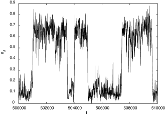
Figure 9: Simulation results for a population history, represented by $n_{J}$ (number of full-phosphorylated particles). We have used a system of $100$ particles and a $g$-value of $4.08$.

IV.1 Diffusion eigenvalues and eigenvectors

We compute the noise spectrum by further expanding Eq. (LABEL:eq:L_varphi_expand) about $\bar{\tilde{\phi}}\equiv 0$, defining $\hat{\phi}\equiv\bar{\hat{\phi}}+{\hat{\phi}}^{{}^{\prime}}$ and letting $\bar{\hat{\phi}}$ be a constant solution to Eq. (42), so that the linear term in $\varphi$ vanishes. Using $\hat{L}\left(0,\bar{\hat{\phi}}\right)=0$, the second-order expansion defines the Gaussian kernel, with the form

$$\hat{L}=\varphi D_{0}{\hat{\phi}}^{{}^{\prime}}+\varphi D_{2}{\varphi}^{T}+\mbox{h.o.}$$ (45)

and higher-order terms (h.o.) are left for perturbative expansion. The diffusion kernel governing ${\hat{\phi}}^{{}^{\prime}}$ in Eq. (45) is

$$D_{0} = {\partial}_{z}+\left(1+g{\bar{\hat{\phi}}}_{0}\right)D_{-}+\left(1+g{\bar{\hat{\phi}}}_{J}\right)D_{+}$$ (46)

$$\mbox{}+g\left(D_{-}\bar{\hat{\phi}}1^{T}P_{-}+D_{+}\bar{\hat{\phi}}1^{T}P_{+}\right),$$

while the kernel controlling the constraint field $\varphi$ is

$$D_{2}=\frac{g}{2}\left\{\left(D_{-}\bar{\hat{\phi}}{\bar{\hat{\phi}}}^{T}P_{-}+D_{+}\bar{\hat{\phi}}{\bar{\hat{\phi}}}^{T}P_{+}\right)+\mbox{transpose}\right\}.$$ (47)

Remarkably, about general normalized solutions to Eq. (7), the kernel (47) has only two nonzero eigenvalues ${\lambda}_{\pm}$, with eigenvectors $v_{\pm}$:

$$D_{2}v_{\pm}=\frac{g}{2}{\lambda}_{\pm}v_{\pm}.$$ (48)

We construct $v_{\pm}$ from convenient, orthonormal “center” and “edge” components,

$${\left(v_{c}\right)}_{j}=\sqrt{\frac{\sinh\left(\xi\right)}{\sinh\left[\left(J-1\right)\xi\right]}}\left(x^{j-J/2}\right),1\leq j\leq J-1,$$ (49)

and zero otherwise, and

$${\left(v_{e}\right)}_{j=\left(J/2\pm J/2\right)}=\frac{\pm x^{\pm\left(\frac{J-1}{2}\xi\right)}}{\sqrt{2\cosh\left[\left(J-1\right)\xi\right]}}$$ (50)

and zero otherwise.

A term that appears in the solution for the eigenvalues is abbreviated

$${\cal R}\left(\xi\right)\equiv\sqrt{1+\tanh\left[\left(J-1\right)\xi\right]\tanh\left(\frac{1}{2}\xi\right)},$$ (51)

in terms of which

$${\lambda}_{\pm}=2\left\{\pm{\cal R}\left(\xi\right)-1\right\}\cosh\left[\left(J-1\right)\xi\right]{\left(\frac{\sinh\left(\frac{1}{2}\xi\right)}{\sinh\left(\frac{J+1}{2}\xi\right)}\right)}^{2},\\$$

and the orthonormal eigenvectors

$$v_{\pm}=\frac{1}{\sqrt{2{\cal R}\left(\xi\right)}}\left\{v_{c}\sqrt{{\cal R}\left(\xi\right)\pm 1}\mp v_{e}\sqrt{{\cal R}\left(\xi\right)\mp 1}\right\}.$$ (52)

For $g\leq g_{c}$, only $\xi=0$ is consistent, and we get ${\lambda}_{+}\equiv 0$,

$${\lambda}_{-}=-{\left(\frac{2}{J+1}\right)}^{2},$$ (53)

with eigenvector $v_{-}=v_{e}$. This algebraic result emphasizes the efficiency of expanding about Poisson backgrounds for weakly perturbed stochastic processes. The only deviation from Poisson which must be handled perturbatively comes from a single mode of $\varphi$, whose fluctuations represent exchanges between $n_{0}$ and $n_{j}$ by Eq. (50). These are of course the noise in the catalytic rates that feeds back into the distribution as a whole.

IV.2 Hubbard-stratonovitch transformation about the symmetric phase

Rather than complete the square in Eq. (45) (á la Onsager and Machlup Onsager:Machlup:53 ), which is cumbersome for one eigenvector, we introduce into Eq. (28) an auxiliary-field representation of unity at each time:

$$1={\cal N}\int{\cal D}\tilde{\zeta}e^{-\frac{N}{2g}\int dz{\tilde{\zeta}}^{2}},$$ (54)

in which ${\cal N}$ is a time- and field-independent normalization. Shifting the auxiliary field $\tilde{\zeta}$ (a symmetry of the measure), we introduce the physical Langevin field $\zeta$ as

$$\tilde{\zeta}\equiv\zeta-g\sqrt{-{\lambda}_{-}}\left(\varphi\cdot v_{-}\right).$$ (55)

The net effect on $\hat{L}$ is the shift

$$\hat{L} \rightarrow \frac{1}{2g}{\tilde{\zeta}}^{2}+\hat{L}$$

$$\approx \frac{1}{2g}{\zeta}^{2}+\varphi\left(D_{0}{\hat{\phi}}^{{}^{\prime}}-\sqrt{-{\lambda}_{-}}v_{-}\zeta\right)+\frac{g}{2}{\lambda}_{+}{\left(\varphi\cdot v_{+}\right)}^{2}.$$

$\zeta$ is $\delta$-correlated in $z$ with weight $g/N$,

$$\left<{\zeta}_{z}{\zeta}_{z^{\prime}}\right>=\frac{g}{N}\delta\left(z-z^{\prime}\right),$$ (57)

and drives the field ${\hat{\phi}}^{{}^{\prime}}$ through the inverse of $D_{0}$, acting on $v_{-}$. In the symmetric phase ${\lambda}_{+}=0$ and this is all there is to the bare noise kernel; in the symmetry-broken phase we must still handle (by other means) the term $\varphi\cdot v_{+}$, which however remains orthogonal to the $v_{-}$ in the Langevin term. Integration over $\varphi$ in the symmetric phase produces

$${\hat{\phi}}^{{}^{\prime}}_{z}=\sqrt{-{\lambda}_{-}}\int_{0}^{z}dz^{\prime}G_{0}\left(z,z^{\prime}\right)v_{-}{\zeta}_{z^{\prime}}$$ (58)

as a field equation to Gaussian order, in which $G_{0}\left(z,z^{{}^{\prime}}\right)$ is defined in terms of Eq. (46) by

$$D_{0}\,G_{0}\!\left(z,z^{\prime}\right)\equiv\delta\left(z-z^{\prime}\right).$$ (59)

Note that from Eq.  58 we see that $\left<{\hat{\phi}}^{{}^{\prime}}_{z}\right>=0$, which implies that there are no corrections to the mean-field result for the expectation value in the symmetric phase.

IV.3 Fluctuations about the symmetric order parameter

As an example we compute to lowest order the fluctuations in the order parameter about the symmetric phase, where the diffusive Green’s function is easy to compute in closed form. Application of the number operators first to the basis $\left|n\right)$ and then to the coherent-states in Eq. (28) yields the connected component of the variance (expressed in descaled fields)

$$\frac{\left<{\left(n_{J}-n_{0}\right)}^{2}\right>-{\left<n_{J}-n_{0}\right>}^{2}}{2N/\left(J+1\right)}=1+N\left(J+1\right)\left<{\left(\frac{{\hat{\phi}}^{{}^{\prime}}_{J}-{\hat{\phi}}^{{}^{\prime}}_{0}}{\sqrt{2}}\right)}^{2}_{z}\right>.$$ (60)

From the field equation (58) and the correlator (57) we obtain the ${\hat{\phi}}^{{}^{\prime}}$ noise

$$\left<{\left(\frac{{\phi}^{{}^{\prime}}_{J}-{\phi}^{{}^{\prime}}_{0}}{\sqrt{2}}\right)}^{2}_{z}\right>=-{\lambda}_{-}\frac{g}{N}\int_{0}^{z}dz^{\prime}{\left(\frac{\left[\begin{array}[]{ccccc}-1&0&\cdots&0&1\end{array}\right]}{\sqrt{2}}\cdot G_{0}\left(z,z^{\prime}\right)\cdot v_{-}\right)}^{2},$$ (61)

and it remains only to compute the mode expansion of the diffusion kernel in $D_{0}$ from Eq. (46) in the uniform background $\bar{\hat{\phi}}=1/\left(J+1\right)$.

The symmetric-phase $D_{0}$ contains a symmetric linear diffusion matrix with endpoint corrections, so its eigenvectors $v_{k}$ have components ${\left(v_{k}\right)}_{j}={\cal N}_{k}\cos\left[{\theta}_{k}+{\kappa}_{k}\left(j-J/2\right)\right]$, with ${\cal N}_{k}$ a normalization. The eigenvalues are immediate on the interior sites,

$${\lambda}_{k}=4\left(1+\frac{g}{J+1}\right){\sin}^{2}\frac{{\kappa}_{k}}{2},$$ (62)

and consistency of the interior with the endpoint corrections then determines ${\kappa}_{k}$ and ${\theta}_{k}$.

Either $\sin\left(J+1\right){\kappa}_{k}/2=0\Rightarrow{\kappa}_{k}=\pi k/\left(J+1\right)$, $k$ even, and ${\theta}_{k}=0$, or $\cos{\theta}_{k}=0\Rightarrow{\theta}_{k}=\pi/2$ and ${\kappa}_{k}$ solves the matching equation

$$\tan\frac{{\kappa}_{k}}{2}=\frac{g}{J+1+2g}\tan\frac{J+1}{2}{\kappa}_{k}.$$ (63)

Eq. (63) is regular for $k\geq 3$ odd, and creates only a small wavenumber shift from the free diffusion solution, leaving ${\kappa}_{k}\approx\pi k/\left(J+1\right)$. The important mode for critical behavior is $k=1$ as $g\rightarrow g_{c}$, where ${\kappa}_{1}\rightarrow 0$ as

$$\frac{{\kappa}_{1}^{2}}{6}\rightarrow\frac{1}{{\left(J+1\right)}^{2}}\left(\frac{1}{g}-\frac{1}{g_{c}}\right).$$ (64)

In terms of these the modal expansion of the free Green’s function is

$$G_{0}\left(z,z^{\prime}\right)=\Theta\!\left(z-z^{\prime}\right)\sum_{k=1}^{J+1}e^{-{\lambda}_{k}\left(z-z^{\prime}\right)}v_{k}v_{k}^{T}.$$ (65)

Only odd-$k$ modes from $G_{0}$ couple to $v_{-}$ in Eq. (61), by symmetry, and the wavenumber sums from $k\geq 3$ are easily approximated with a two-dimensional $k$ integral. We note that for all these modes ${\cal N}_{k}^{2}\approx 2/\left(J+1\right)$, and the only values that contribute to the inner product come from $j=\pm J/2$, giving ${\sin}^{2}\!\left({\kappa}_{k}J/2\right)\approx 1$. Thus the nonsingular modes in the diffusion kernel provide a smooth background approximately linear in $g$.

The leading contribution from the $k=1$ mode occurs when it is present in both factors of $G_{0}$. For small $g-g_{c}$ this mode is almost linear in $j$, with normalization ${\cal N}_{1}^{-2}\rightarrow{\kappa}_{1}^{2}\sum_{j=-J/2}^{J/2}j^{2}$. Evaluating this singular term separately, with Eq. (62) for the eigenvalue and Eq. (64) for the limiting value of the wavenumber, and then combining with the background from the regular modes, we obtain the approximation

$$\frac{\left<{\left(n_{J}-n_{0}\right)}^{2}\right>-{\left<n_{J}-n_{0}\right>}^{2}}{2N/\left(J+1\right)}\approx 1+\frac{8g}{\pi}\frac{\log\left(J+1\right)}{\left(J+1\right)}+{\cal C}\frac{6}{J+1}\frac{g^{2}}{\left(1+\frac{g}{J+1}\right)\left|g-g_{c}\right|}.$$ (66)

It is convenient to separate the constant

$${\cal C}=\frac{{\left(J+1\right)}^{3}}{J^{2}\left(J-1\right)}{\left(\frac{12}{J}\sum_{j=-J/2}^{J/2}{\left(\frac{j}{J}\right)}^{2}\right)}^{-2}$$ (67)

from the discrete sum for the $k=1$ norm, because ${\cal C}\rightarrow 1$ at large $J$, but differs somewhat at the smaller $J$ of more likely biological interest.

The approximation (66) to the closed-form mode expansion for the variance of the order parameter is compared to numerical simulations in Fig. 10. We have continued the analytic expression through the critical point to show the peak, though the character of the modes rapidly changes as the distribution becomes skewed in the symmetry-broken phase. A similar mode expansion exists in this phase, but requires the relaxation eigenvectors and eigenvalues for asymmetric diffusion. We have not computed these in closed form, and do not pursue them numerically because in the symmetry-broken phase fluctuations quickly come to be dominated by the center-of-mass behavior we derive below in Eq. (69).

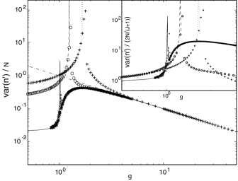
Figure 10: Fluctuations in the order parameter scaled for $g$ above and below critical. $\mbox{\em var}\left(n^{\prime}\right)$ stands for the variance $\left<{\left(n_{0}-n_{J}\right)}^{2}\right>-{\left<n_{0}-n_{J}\right>}^{2}$. Lines are leading-order expansion of Eq. (66) in fluctuations about the symmetric mean-field solution, continued through $g_{c}$; symbols from simulation, $J+1$ values and markers as in Fig. 8. Large panel shows convergence of $\mbox{\em var}\left(n^{\prime}\right)$ to $N/g$ at all $J$. Inset shows convergence of $\mbox{\em var}\left(n^{\prime}\right)$ to Poisson result $2N/\left(J+1\right)$ as $g\rightarrow 0$.

Three main observations are important. First, the singularity in the variance has the leading-order approximation

$$\frac{\left<{\left(n_{J}-n_{0}\right)}^{2}\right>-{\left<n_{J}-n_{0}\right>}^{2}}{2N/\left(J+1\right)}\approx\frac{\mbox{const}\sim 1}{\left(J+1\right)\left|g-g_{c}\right|},$$ (68)

comparable to that of the mean-field Ising ferromagnet, like the scaling of the order parameter. The variance has weight $1/\left(J+1\right)$, because the lowest diffusive mode, corresponding to the average magnetization, is the only collective fluctuation participating in the phase transition near the critical point.

Second, we see that the weak-coupling scaling of $\left<{\left(n_{J}-n_{0}\right)}^{2}\right>-{\left<n_{0}-n_{J}\right>}^{2}$ is that of Poisson noise for an average of $N/\left(J+1\right)$ particles per site. (This is shown in the inset of Fig. 10.)

Third – and the reason we do not pursue the low-order expansion for the symmetry-broken-phase two-point function – we see that for $g\gg g_{c}$ the variance $\left<{\left(n_{J}-n_{0}\right)}^{2}\right>-{\left<n_{0}-n_{J}\right>}^{2}$ goes to a universal form $N/g$ for any $J$. The independence of this scaling regime from $J$ indicates that the particles interact with one end of the chain and the exogenous catalysis only, suggesting a strong-coupling limit.

In addition, for large $J$, the center-of-mass equation (3) predicts (for $I=P$), in steady state for the symmetry-broken phase, that the variance will equal

$$~{}\left<n_{e}\right>N\left[1-\frac{1}{g}-\frac{\left<n_{e}\right>}{N}\right]$$ (69)

where $n_{e}$ signifies whichever of the end sites $0$ or $J$ is occupied (which depends on which of the two bistable states is chosen). In Fig. 11 we plot the simulation data for the variance for $J+1=100$ against the estimate from Eq. (69). For the value of $\left<n_{e}\right>$, we simply take the value of the order parameter at the corresponding value of $g$. As we see, this explains the form of the fluctuation spectrum for large J very well. The fact that we are able to replace the order parameter $\left|\left<n_{J}-n_{0}\right>\right|$ by $n_{e}$ demonstrates that this scaling regime is independent of $J$ as well and the particles only interact with one end of the chain all through the symmetry-broken phase.

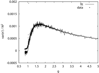
Figure 11: The fluctuation in the order parameter for $J+1=100$ and $N=400$ is plotted against the fit predicted by Eq.  69.

V Large excursions

From the $1/g$ scaling of the Lagrangian term for the Langevin field in Eq. (LABEL:eq:L_Langevin_shift) and the presence of unstable eigenvalues in the fluctuation kernel (45) about static stationary backgrounds, we anticipate that perturbation theory containing fluctuations associated with domain flips will not converge Cardy:Instantons:78 , and that the rates for these large excursions will be computed as an essential singularity with respect to the perturbation expansion. The remarkable similarity to Hamiltonian dynamical systems created by this method for treating generating functions reduces the problem of estimating both escape trajectories and first passage times to that of identifiying the heteroclinic network Gluckheimer:het_cycles:88 ; Gluckheimer:dyn_sys:02 in the associated dynamical system.

We construct the expansion appropriate to the second-order transitions, beginning with the analysis of the exact stationary points corresponding to solutions of the classical diffusion equation from arbitrary initial conditions. From the structure of these solutions, we identify the “approximate stationary points” associated with domain flips, and compute the trajectory and action for a low-dimensional example numerically. Comparisons to simulation suggest that this calculation correctly predicts the leading exponential dependence on particle number of the residence time in domains in the symmetry-broken phase.

V.1 The expansion in semiclassical stationary points

We define the stationary-point expansion of the path integral (28) implicitly by the requirement that the residual perturbation theory converge. In principle we must include not only the (generally unique) exact stationary point specified by the initial state $\left|{\psi}_{0}\right)$, but also a sufficient set of “approximate” stationary points associated with states that converge exponentially fast toward $\left|{\psi}_{0}\right)$, with respect to prediction of late-time observables. In this representation using generating functionals for probability distributions over spaces of histories, a “stationary point” refers to any full path $\left(\bar{\tilde{\phi}},\bar{\hat{\phi}}\right)$ satisfying the classical condition that the linear variations of $L$ (including time-derivative terms) vanish:

$$\frac{\partial L}{\partial{\tilde{\phi}}}=0;\mbox{ }\frac{\partial L}{\partial\phi}=0.$$ (70)

If $\tilde{\phi}=0$, the solution of Eq. (42) solves the above to recover the mean-field solutions; in this section we relax the requirement $\tilde{\phi}=0$ to uncover a larger set of solutions which result in a nonzero value for $L$.

Formally, then, the removal of the stationary-point contribute leads to the functional form

$$\left(0\right|\exp\left(\sum_{j}a_{j}\right)\left|{\psi}_{t}\right)=$$

$$\sum_{\bar{\tilde{\phi}},\bar{\hat{\phi}}}e^{-N\int\,dz\bar{\hat{L}}}\int{\cal D}\varphi\,{\cal D}{\hat{\phi}}^{{}^{\prime}}e^{-N\int dz\left(\hat{L}-\bar{\hat{L}}\right)}e^{{\tilde{\phi}}_{0}\cdot\left(\bar{n}-{\phi}_{0}\right)},$$

where $\bar{\hat{L}}$ denotes $\hat{L}\!\left(\bar{\tilde{\phi}},\bar{\hat{\phi}}\right)$. As perturbative corrections scale as powers of $1/N$, by Eq. (61), to leading order we will treat $\hat{L}-\bar{\hat{L}}$ as a quadratic form in $\varphi$ and ${\hat{\phi}}^{{}^{\prime}}$, of the form (45), now about more general time-dependent backgrounds.

The formal sum $\sum_{\bar{\tilde{\phi}},\bar{\hat{\phi}}}$ is properly a discrete sum in the number $n\in 0,\ldots,\infty$ of domain flips, of a time-ordered integral over their positions $\left\{z_{1},\ldots,z_{n}\right\}$. The integral is necessary Coleman:AoS:85 , because as the domain flips converge toward true stationary points, the fluctuation generated by time translation of any solution becomes a null eigenvector of the functional determinant about that solution. (This is a variant on Goldstone’s theorem Weinberg:QTF_II:96 , associated with the time-translation symmetry spontaneously hidden by the instanton Smith:evo_games:11 .) This eigenvector is replaced by the integral (with a Jacobean), and the remaining functional determinant is a product of positive eigenvalues, by construction.

We will check that the transition times of the instantons are finite and that they converge exponentially to the static backgrounds, so that when they are improbable the dilute-gas sum is well defined. As we verify below, the classical solutions all have $\bar{\tilde{\phi}}\equiv 0$ and zero action, and we denote by $S_{0}$ the action $N\int dz\bar{\hat{L}}$ associated with a single instanton. Letting $1/{\zeta}_{0}$ denote the Jacobean relating the null eigenvalue to the measure for $z$-translation of the instanton, we recast the sum in Eq. (LABEL:eq:funct_int_rep_sp_exp) as

$$\left(0\right|\exp\left(\sum_{j}a_{j}\right)\left|{\psi}_{t}\right)=\sum_{n=0}^{\infty}\frac{e^{-nS_{0}}}{n!}{\bf T}\int\frac{dz_{1}}{{\zeta}_{0}},\ldots,\int\frac{dz_{n}}{{\zeta}_{0}}\int{\cal D}\varphi\,{\cal D}{\hat{\phi}}^{{}^{\prime}}e^{-N\int dz\left(\hat{L}-\bar{\hat{L}}\right)}e^{{\tilde{\phi}}_{0}\cdot\left(\bar{n}-{\phi}_{0}\right)},$$ (72)

in which ${\bf T}$ denotes time-ordering in $z$ of the positions of the instantons. The presence of $n$ factors of $1/{\zeta}_{0}$ in the $n$-instanton determinant follows from the product structure of functional determinants and the wide separation of finite supports in $z$ where the background differs from that of a steady state Coleman:AoS:85 .

Like the computation of the energy shift in the equilibrium double-well problem, we see that observables relating to persistence within a domain will receive contributions from the even terms in the sum over $n$, while those relating to domain flips will receive contributions from the odd terms. The likelihood of persistence decays exponentially in $z$ at early times with rate

$$r_{\mbox{\scriptsize flip}}=\frac{1}{{\zeta}_{0}}e^{-S_{0}}.$$ (73)

The computation of the instanton action $S_{0}$, which is responsible for the leading exponential dependence of $r_{\mbox{\scriptsize flip}}$ is most easily carried out within the complete analysis of the semiclassical stationary points, beginning with the classical diffusion solutions.

V.2 Action-angle variables and the structure of the Hamiltonian

The equations of motion (37,38) in $\bar{\tilde{\phi}}$ and $\bar{\hat{\phi}}$ do not directly give the evolution of the physical particle numbers, or efficiently use the symmetries of Sec. III.4. To do both, it is convenient to transform the background fields as ${\bar{{\phi}^{\dagger}}}_{j}\equiv e^{{\sigma}_{j}}$, and ${\bar{\hat{\phi}}}_{j}\equiv{\nu}_{j}e^{-{\sigma}_{j}}$. ${\nu}_{j}$ is then the semiclassical approximation to the relative number $\left<n_{j}\right>/N$. This change of variables is equivalent to an action-angle transformation in classical mechanics Goldstein:ClassMech:01 , and we check in Ref. Smith:evo_games:11 that as well as producing a more convenient form for the action, it leads to the correct measure for fluctuations. The Lagrangian (34) retains a simple kinetic term, up to a total derivative:

$$\bar{\hat{L}}=\sigma\cdot{\partial}_{z}\nu+\hat{\Omega}\left(\sigma,\nu\right),$$ (74)

and the equations of motion in the new variables become, respectively,

$${\partial}_{z}{\nu}_{j}=-\frac{\partial\hat{\Omega}}{\partial{\sigma}_{j}},$$ (75)

and

$${\partial}_{z}{\sigma}_{j}=\frac{\partial\hat{\Omega}}{\partial{\nu}_{j}}.$$ (76)

With the interpretation of the number field $\nu$ as a position, and $\sigma$ its canonically conjugate momentum, $-\hat{\Omega}$ becomes the correctly signed Hamiltonian for classical solutions. The conservation law $d\hat{\Omega}/dz=0$ is mathematically a conservation of energy, but the particular value $\hat{\Omega}\equiv 0$ associated with all stationary points initiated by classical distributions is a distinctive feature of this stochastic-process application of Hilbert-space methods.

The global symmetry whose Noether charge is total number becomes immediate in action-angle variables. Defining

$$\bar{\sigma}\equiv\frac{1}{J+1}\sum_{j=0}^{J}{\sigma}_{j},$$ (77)

the Lagrangian becomes

$$\hat{L} = \bar{\sigma}{\partial}_{z}\left(\sum_{j=0}^{J}{\nu}_{j}\right)$$

$$\mbox{}+\sum_{j=0}^{J}\left({\sigma}_{j}-\bar{\sigma}\right){\partial}_{z}{\nu}_{j}+\hat{\Omega}\left(\sigma,\nu\right),$$

in which $\bar{\sigma}$ multiples the $z$-derivative of conserved total number in the first line, and only differences ${\sigma}_{i}-{\sigma}_{j}$ appear in either the kinetic term or the $\hat{\Omega}$ of the second line.

To expose the structure of the associated dynamical system, and to make the terms in it readily visualizable from the mean-field diffusive solutions, we perform a final transformation by introducing the log ratio of particle fluxes between sites $j$ and $j+1$,

$$r_{j+1,j}\equiv\frac{1}{2}\log\left[\frac{\left(1+g{\nu}_{J}\right){\nu}_{j}}{\left(1+g{\nu}_{0}\right){\nu}_{j+1}}\right].$$ (79)

In terms of these the $\sigma$-dependence of $\hat{\Omega}$ may be simplified to read

$$\hat{\Omega}\left(\sigma,\nu\right)=2\sqrt{\left(1+g{\nu}_{0}\right)\left(1+g{\nu}_{J}\right)}\sum_{j=0}^{J-1}\left\{\sqrt{{\nu}_{j+1}{\nu}_{j}}\left[\cosh\left(r_{j+1,j}\right)-\cosh\left({\sigma}_{j}-{\sigma}_{j+1}-r_{j+1,j}\right)\right]\right\}.$$ (80)

The one-dimensional geometry we have assumed for the graph of phosphorylation and dephosphorylation transitions makes possible the definition of a function $\sigma\!\left(\nu\right)$ at each number configuration, satisfying

$${\sigma}_{j+1}\!\left(\nu\right)-{\sigma}_{j}\!\left(\nu\right)=-r_{j+1,j},$$ (81)

(up to a convention for specifying $\bar{\sigma}$ at each $\nu$, which we may take to be arbitrary). $\sigma\!\left(\nu\right)$ is a reference point for the canonical momentum coordinate $\sigma$, and $\sigma-\sigma\!\left(\nu\right)$ functions as the kinematic momentum for this system.

We may see this by introducing the Hamiltonian potential function

$$V\!\left(\nu\right)=2\sqrt{\left(1+g{\nu}_{0}\right)\left(1+g{\nu}_{J}\right)}\sum_{j=0}^{J-1}\sqrt{{\nu}_{j+1}{\nu}_{j}}\left[\cosh\left(r_{j+1,j}\right)-1\right],$$ (82)

in terms of which

$$-\hat{\Omega}\left(\sigma,\nu\right)=2\sqrt{\left(1+g{\nu}_{0}\right)\left(1+g{\nu}_{J}\right)}\sum_{j=0}^{J-1}\sqrt{{\nu}_{j+1}{\nu}_{j}}\left\{\cosh\left[{\left(\sigma-\sigma\!\left(\nu\right)\right)}_{j}-{\left(\sigma-\sigma\!\left(\nu\right)\right)}_{j+1}\right]-1\right\}-V\!\left(\nu\right).$$ (83)

To leading order the explicit $\cosh$ in Eq. (83) is simply a quadratic form in $\sigma-\sigma\!\left(\nu\right)$, with a matrix of inverse masses defined by the remaining square-root terms. When $\sigma-\sigma\!\left(\nu\right)=0$, Eq. (75) shows that ${\partial}_{z}\nu=0$, verifying the interpretation of $\sigma-\sigma\!\left(\nu\right)$ as the kinematic momentum. Furthermore, if this kinematic momentum vanishes at any local minimum of $V\!\left(\nu\right)$, Eq. (76) shows that ${\partial}_{z}\sigma=0$, hence ${\partial}_{z}\left(\sigma-\sigma\!\left(\nu\right)\right)=0$. The local minima satisfy $V\!\left(\nu\right)=0$ and are attained only when each $r_{j+1,j}=0$ independently, because the $\cosh$ terms in Eq. (82) are never negative. These are of course exactly the (stable and saddle-point) mean-field solutions with particle exchange between adjacent sites obeying detailed balance. We identify them in graphs below as the fixed points of the classical diffusion equation.

It can be shown Smith:evo_games:11 that, as long as the quadratic expansion in $\sigma$ is a good approximation, and as long as the effective mass terms implicit in Eq. (83) are not a strong function of $\nu$ (which we will verify), all stationary points of the action closely approximate ordinary mechanical trajectories in the potential $-V\!\left(\nu\right)$, with position coordinate $\nu$ and kinematic momentum $\sigma-\sigma\!\left(\nu\right)$. For the classical solutions $\sigma\equiv 0$, shown in Fig. 12, the unbounded trajectories are those that originate in non-equilibrium initial conditions and converge exponentially slowly on the saddle or stable fixed points. The two bounded trajectories, between the saddle and either stable fixed point, travel along the saddle path of the potential, $-V\!\left(\nu\right)$, which is bounded above by 0 and unbounded below, and make up part of the heteroclinic network Gluckheimer:het_cycles:88 ; Gluckheimer:dyn_sys:02 of the associated hyperbolic system.

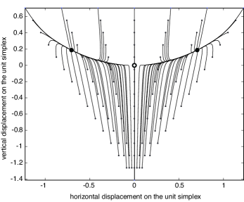
Figure 12: Classical flowfield of the particle numbers ${\nu}_{j}$ for $J=2$, shown on the simplex $\sum_{j=0}^{2}{\nu}_{j}\equiv 1$. Upper left corner is $n_{0}=1$, upper right corner is $n_{2}=1$, and bottom is $n_{1}=1$. Dots are a selection of initial conditions, and classical diffusion solutions are the flowlines emanating from them. The uniform distribution ${\nu}_{j}=1/3$ (open circle) is the saddle point, and the stable fixed points (heavy dots) are attractors.

For ordinary mechanical flow, we know that the full heteroclinic network consists of trajectories running both ways between the stable and saddle fixed points. If this were a purely mechanical system, the reverse trajectories would be strict time-reversal images of the bounded classical diffusion trajectories. (Note that an exact reversal $\left({\sigma}_{j}-{\sigma}_{j+1}\right)\rightarrow 2r_{j+1,j}-\left({\sigma}_{j}-{\sigma}_{j+1}\right)$ would also leave $\hat{\Omega}=0$.) Here, a small $\nu$-dependence of the effective mass terms causes them to differ slightly from each other and from the saddle path over $-V\!\left(\nu\right)$.

In Fig. 13, we directly compute the trajectory of the reverse bounded path, by integration along the saddle instability of the equations of motion (75,76). The fact that it nearly retraces the classical diffusive direction of slowest flow checks the approximation that both trajectories are dominated by the potential $-V\!\left(\nu\right)$ itself.

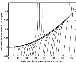
Figure 13: Flowfield of the instanton solution in $J=2$, for values $\xi=1$, so $g\approx 4.0862$. Fine lines are classical diffusion solution from Fig. 12, and bold line is the instanton.

For an instanton in a classical equilibrium field theory, the conjugate and the kinematic momentum would be the same quantity. Both forward and reverse trajectories along the saddle path in the potential $-V\!\left(\nu\right)$ would have locally minimum but non-zero action, and in that sense both would be “non-classical” trajectories Coleman:AoS:85 . The distinctive feature of the path integrals associated with master equations of the form we have considered here is the offset $\sigma\!\left(\nu\right)$ from the canonical momentum that appears in the kinetic term of the Lagrangian (74) to the kinematic momentum. This offset is responsible for $S\equiv 0$ for all diffusion solutions, including the bounded trajectories from saddle to stable fixed points, and it approximately doubles the value of the Lagrangian (74) along the reverse trajectories. The value of this Lagrangian, along the numerically determined path of Fig. 13, is shown in Fig. 14. Like the Lagrangian for a classical problem, it is positive definite, and approximates the WKB integral for barrier escape, except with an extra factor of 2: $S\approx 2N\int\sqrt{d{\nu}^{T}md\nu}\sqrt{2V\!\left(\nu\right)}$, where $d\nu$ is a length element on the coordinate $\nu$, and $m$ is the matrix of effective mass values implied by Eq. (83). This approximate form follows simply from the nearly time-reverse character of escapes versus classical paths of slowest-diffusion, and may be derived from the original Gaussian-order approximation to such escapes by Onsager and Machlup Onsager:Machlup:53 . Readers seeking a systematic derivation, including the Onsager-Machlup small-fluctuation approximation, may find these in Ref. Smith:LDP_SEA:11 or Ref. Smith:evo_games:11 .

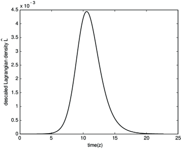
Figure 14: Linear-scale plot of the Lagrangian density per particle $\bar{\hat{L}}$ of the instanton trajectory. A logarithmic plot of the same quantity (not shown) demonstrates exponential decay toward zero at early and late times.

For the parameter values of Fig. 13, the integral $\int dz\bar{\hat{L}}$ under the curve of Fig. 14 converges to a value near $0.0206$. Fig. 15 compares numerical estimates of the residence time in this model, inverse to the rate $r_{\mbox{\scriptsize flip}}$ of Eq. (73), to particle number $N$. The slope of the logarithm of $1/r_{\mbox{\scriptsize flip}}$ should be $dS_{0}/dN=\int dz\bar{\hat{L}}$, up to corrections decaying as $1/N$, and we observe quantitative agreement with the numerical estimate of the instanton to $\sim 10\%$.

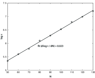
Figure 15: Plot comparing residence times to particle number for the parameters of Fig. 14. Slope of numerical estimates, which should correspond to $dS_{0}/dN=\int dz\bar{\hat{L}}$ is best fit by $0.023$, while direct integration under the curve of Fig. 14 yields $0.0206$.

Although we do not pursue the analytic forms in this paper, the dependence of the coefficient of $N$ (giving decay times) on number of sites $J$ and the distance from criticality $g-g_{C}$ may also be found from simulations. Fig. 16 symmarizes these numerical results, showing that the dependence on small-integer $J$ is roughly linear, and the dependence on $g-g_{C}<1$ is weakly nonlinear.

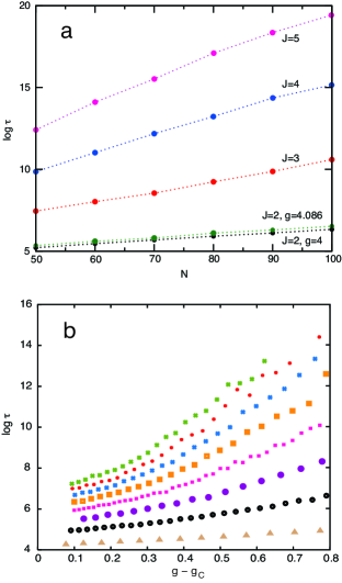
Figure 16: Plot of expected residence times $\tau$ from simulations in the symmetry-broken state as functions of $J$, $N$, and distance of the coupling strength from its critical value, $g-g_{C}$. (a): $\log\tau$ vs. $N$ for $J\in\left\{2,\ldots,5\right\}$. In simulations $I\equiv P$, $g=N/\sqrt{IP}$ is held constant, and $g-g_{C}$ is held equal to 1. Green curve for $J=2$ and $g=4.0862$ corresponds to the value $\xi\equiv 1$, which we have computed analytically, corresponding to the coefficient $d\log\tau/dN$ shown in Fig. 15. (b): $\log\tau$ vs. $g-g_{C}$ for values $J\in\left\{2,\ldots,9\right\}$ (from bottom to top) at $N=50$.

V.3 Summary of semiclassical results

We have seen that the classical “action” for this reaction-diffusion theory, once constructed, yields quite nicely the two extremes of behavior of interest in cooperative intermolecular phase transitions. The classical stationary points coincide exactly with the usual mass-action differential equations. Corrections to these from cubic and higher-order fluctuation effects are readily incorporated (for an example, see Ref. Smith:evo_games:11 ), but to the resolution of our simulations, we cannot identify a need for such corrections at these parameter values, so we have not pursued them.

The nonclassical stationary trajectories are the projection from this $\left(2J+2\right)$-dimensional configuration space, onto the one-dimensional path most likely to destabilize the symmetry-broken phase, which closely approximates the path of slowest diffusive correction. The methods shown here therefore provide a compact and convenient way to estimate the escape trajectories and first-passage times for even quite richly structured nonlinear diffusion processes of this kind. These methods, originally developed for applications to reaction-diffusion theory, are increasingly finding applications in epigenetics Aurell:epigenetics:02 ; Roma:epigenetics:05 and systems biology Sinitsyn:CG_chem_nets:09 where particle numbers may be small, making fluctuation effects important, while at the same time the structure of the state space remains complex to describe.

The reduction to a one-dimensional system was assumed given, in the treatment in Ref. Bialek:memory:01 of a switching system comparable to ours; we have shown here a systematic approach to estimating such escape trajectories. We have also verified that the action of the instanton, easily numerically integrated once the trajectory is found, produces both the correct $N$ scaling, and good quantitative agreement, with the domain residence times. We expect that, while the treatment of the functional determinant will be more difficult for metastable domains in first-order transitions, the classical-level analysis comparable to ours will be similar, and roughly as effective.

VI Discussion and conclusions

We have tried to idealize in a reasonable way a large class of biomolecular signal transduction systems, and to apply the most complete formalism available to decompose and quantitatively estimate their properties as switches. Our results thus combine a number of technical advances in recognized domains, with several conceptual insights relevant to the robustness and evolution of devices. Of necessity in a short treatment, our idealizations of feedback and single timescales for all microscopic motion have abstracted away from some important problems of connection with phenomenological models of real regulatory protein systems.

VI.1 Technical advances

The operator treatments of gene-expression switching Sasai:gene_exp:03 extended traditional mass-action models to include perturbative noise from first principles. We have further extended the operator methods to a path-integral treatment, which adds an intuitive and computationally tractable approach to large deviations.

We have demonstrated that expansion of weakly nonlinear stochastic processes about Poisson backgrounds leads to very efficient perturbative schemes for correcting the full probability distribution (not very surprising in retrospect), and that in our particular idealized model, the entire noise spectrum is driven by a single bare Langevin field (perhaps somewhat more surprising, and not noticed before).

Finally, we have shown that the nonlinear projection of the full master equation onto the dominant trajectory participating in domain flips approximately, but not exactly, reverses the unique trajectory of slowest diffusive correction in the classical flow. We have recovered the exponential in $N$ characteristic of extensive large-deviations scaling Touchette:large_dev:09 , and shown how to estimate the exact coefficient to refine the bounds of order unity that are conventionally (and usually correctly) assumed in pure scaling arguments Bialek:memory:01 .

VI.2 Biological insights

The most concrete of our results for biologists seeking to understand the function of signal-transduction cascades and switches is that particle number ($N$), as well as exogenous kinase ($I$) and phosphatase ($P$) numbers, can be used to control the onset of switching, and in cases of asymmetric topology, also the preferred domain of the switch. The control through $N$ offers a feedback from gene expression into the function of the cascade, which apparently has not been considered earlier.

We have demonstrated through the mode expansion in the neighborhood of the phase transition, that only the lowest-eigenvalue collective fluctuation of the diffusion operator induces the instability to symmetry breaking, and scales the divergence in the noise spectrum. For large $J$, we can also predict fluctuations in the symmetry-broken phase because of a simplification induced by the fact that the system senses only one boundary in the entire symmetry-broken phase. This enables us to simplify an exact equation for the center-of-mass of the system to predict fluctuations.

More abstractly, we have distinguished a mechanism for switching based purely on population-level polarization of the protein pool, from mechanisms which depend on limiting one or more transition rates through restrictions on catalytic kinetics. Polarization-based mechanisms make the function of the switch dependent on its catalytic topology and concentrations, but not on kinetic factors, a separation that has been proposed as a route to modularity. We hope that such distinctions can at some point be incorporated in evolutionary models that make quantitative use of the structure of phenotypically neutral networks, where we hope they will explain at least part of the ubiquity of multiple phosphorylation and nonspecific catalysis in cascades of the type we have considered.

VII Acknowledgements

DES thanks Insight Venture Partners for support of this work. SK was supported by the swedish research council.

References

- (1) J. von Neumann. Probabilistic logics and the synthesis of reliable organisms from unreliable components. Automata Studies, 34:43–, 1956.
- (2) G. von Dassow, E. Meir, E. M. Munro, and G. M. Odell. The segment polarity network is a robust developmental module. Nature, 406:188, 2000.
- (3) H. M. Sauro. The computational versatility of proteomic signaling networks. Current Proteomics, 1:67, 2004.
- (4) J. E. Jr. Ferrell. Xenopus oocyte maturation: new lessons from a good egg. Bioessays, 21:833, 1999.
- (5) J. E. Jr. Ferrell. Building a cellular switch: more lessons from a good egg. Bioessays, 21:866, 1999.
- (6) J. J. Tyson, A. Csikasz-Nagy, and B. Novak. The dynamics of cell cycle regulation. Bioessays, 24:1095, 2002.
- (7) M. Sasai and P. Wolynes. Stochastic gene expression as a many-body problem. Proc. Nat. Acad. Sci. USA, 100:2374–2379, 2003.
- (8) A. Goldbeter and D. E. Koshland. An amplified sensitivity arising from covalent modification in biological systems. Proc. Nat. Acad. Sci. USA, 78:6840–6844, 1981.
- (9) C. Y. Huang and J. E. Jr. Ferrell. Ultrasensitivity in the mitogen-activated protein kinase cascade. Proc. Nat. Acad. Sci. USA, 93:10078, 1996.
- (10) J. J. Tyson, K. C. Chen, and B. Novak. Sniffers, buzzers, toggles and blinkers: dynamics of regulatory and signaling pathways in the cell. Curr. Opin. Cell Biol., 15:221, 2003.
- (11) J. E. Ferrell and W. Xiong. Bistability in cell signaling: How to make continuous processes discontinuous, and reversible processes irreversible. Chaos, 11:227, 2001.
- (12) J. E. Lisman. A mechanism for memory storage insensitive to molecular turnover: a bistable autophosphorylating kinase. PNAS, 82:3055, 1985.
- (13) W. Bialek. Stability and noise in biochemical switches. In T. K. Leen, T. G. Dietterich, and V. Tresp, editors, Advances in Neural Information Processing, Cambridge, 2001. MIT Press.
- (14) D. Kültz and M. Burg. Evolution of osmotic stress signaling via map kinase cascades. J. Exp. Biol., 201:3015, 1998.
- (15) Jeremy Gunawardena. Multisite protein phosphorylation makes a good threshold but can be a poor switch. Proc. Nat. Acad. Sci. USA, 102:14617–14622, 2005.
- (16) Salazar, C. and Höfer, T. Versatile reglation of multisite protein phosphorylation by the order of phosphate processing and protein-protein interactions. FEBS journal, 274:1046–1061, 2007.
- (17) A. Kreegipuu, N. Blom, and S. Brunak. Phosphobase, a database of phosphorylation sites: release 2.0. Nucleic Acids Res., 27:237, 1999.
- (18) N. I. Markevich, J. B. Hoek, and B. N. Kholodenko. Signaling switches and bistability arising from multisite phosphorylation in protein kinase cascades. J. Cell Biol., 164:353–359, 2004.
- (19) G. Craciun, Y. Tang, and M. Feinberg. Understanding bistability in complex enzyme-driven reaction networks. Proc. Nat. Acad. Sci. USA, 103:8697–8702, 2006.
- (20) L. W. Ancel and W. Fontana. Plasticity, evolvability and modularity in rna. J. Exp. Zool. (Mol. Dev. Evol.), 288:242–283, 2000.
- (21) W. Fontana. Modeling ‘evo-devo’ with rna. Bioessays, 24:1164–1177, 2002.
- (22) K. Takahasi, S. Tanase-Nicola, and P. Rein ten Wolde. Spatio-temporal correlations can drastically change the response of a mapk pathway. PNAS, 107:2473–2478, 2010.
- (23) B. N. Kholodenko. Negative feedback and ultrasensitivity can bring about oscillations in the mitogen-activated protein kinase cascades. Eur. J. Biochem, 267:1583–1588, 2000.
- (24) R. Heinrich, B. G. Neel, and T. A. Rapoport. Mathematical models of protein kinase signal transduction. Mol. Cell., 9:957–970, 2002.
- (25) X. Wang, N. Hao, H. G. Dohlman, and T. C. Elston. Bistability, stochasticity and oscillations in the mitogen-activated protein kinase cascade. Biophys. J., 90:1961–1978, 2006.
- (26) Orsolya Kapuy, Debashis Barik, Maria Rosa Domingo Sananes, John J. Tyson, and Béla Novák. Bistability by multiple phosphorylation of regulatory proteins. Prog. Biophys. Mol. Biol., 100:47–56, 2009.
- (27) B. Novak, Z. Pataki, A. Ciliberto, and J. J. Tyson. Mathematical model of the cell division cycle of fission yeast. Chaos, 11:277, 2001.
- (28) J. Paulsson and M. Ehrenberg. Noise in a minimal regulatory network: plasmid copy number control. Q. Rev. Biophys., 34:1, 2001.
- (29) Supriya Krishnamurthy, Eric Smith, David C. Krakauer, and Walter Fontana. The stochastic behavior of a molecular switching circuit with feedback. Biology Direct, 2:13, 2007. doi:10.1186/1745-6150-2-13.
- (30) J. E. Ferrell and R. R. Bhatt. Mechanistic studies of the dual phosphorylation of mitogen-activated protein kinase. J. Biol. Chem., 272:19008–19016, 1997.
- (31) W. R. Burack and T. W. Sturgill. The activating dual-phosphorylation of mapk by mek is nonprocessive. Biochemistry, 36:5929–5933, 1997.
- (32) S. Gaudet, K. A. Janes, J. Albeck, E. A. Pace, D. A. Lauffenburger, and P. K. Sorger. A compendium of signals and responses triggered by prodeath and prosurvival cytokines. Mol. Cell Proteomics, 10:1569–1590, 2005.
- (33) M. Kravanja, R. Engelmann, V. Dossonnet, M. Blüggel, H. E. Meyer, R. Frank, A. Galinier, J. Deutscher, N. Schnell, and W. Hengstenberg. The hprk gene of enterococcus faecalis encodes a novel bifunctional enzyme: the hpr kinase/phosphatase. Mol. Microbiol., 31:59–66, 1999.
- (34) A. J. Ninfa. Protein phosphorylation and the regulation of cellular processes by the homologous two-component regulatory systems of bacteria. Genet. Eng., 13:39–72, 1991.
- (35) Sidney Coleman. Aspects of symmetry. Cambridge, New York, 1985.
- (36) Daniel C. Mattis and M. Lawrence Glasser. The uses of quantum field theory in diffusion-limited reactions. Rev. Mod. Phys, 70:979–1001, 1998.
- (37) Gregory L. Eyink. Action principle in nonequilibrium statistical dynamics. Phys. Rev. E, 54:3419–3435, 1996.
- (38) J. Cardy. Field theory and non-equilibrium statistical mechanics. 1999. http://www-thphys.physics.ox.ac.uk/users/JohnCardy/home.html.
- (39) Eric Smith. Large-deviation principles, stochastic effective actions, path entropies, and the structure and meaning of thermodynamic descriptions. Rep. Prog. Phys., 74:046601, 2011. http://arxiv.org/submit/199903.
- (40) N. A. Sinitsyn, Nicalas Hengartner, and Ilya Nemenman. Adiabatic coarse-graining and simulations of stochastic biochemical networks. Proc. Nat. Acad. Sci. USA, 106:10546–10551, 2009.
- (41) Daniel T. Gillespie. Why quantum mechanics cannot be formulated as a markov process. Phys. Rev. A, 49:1607–1612, 1994.
- (42) E. Aurell and K. Sneppen. Epigenetics as a first exit problem. Phys. Rev. Lett., 88:048101:1–4, 2002.
- (43) Hugo Touchette. The large deviation approach to statistical mechanics. Phys. Rep., 478:1–69, 2009. arxiv:0804.0327.
- (44) David Marin Roma, Ruadhan A. O’Flanagan, Andrei E. Ruckenstein, and Anirvan M. Sengupta. Optimal path to epigenetic switching. Phys. Rev. E, 71:011902:1–5, 2005.
- (45) Eric Smith and Supriya Krishnamurthy. Symmetry and collective fluctuations in evolutionary games. 2011. SFI working paper #11-03-010.
- (46) Steven Weinberg. The quantum theory of fields, Vol. II: Modern applications. Cambridge, New York, 1996.
- (47) J. L. Cardy. Electron localisation in disordered systems and classical solutions in ginzburg-landau field theory. J. Phys. C, 11:L321 – L328, 1987.
- (48) L. Onsager and S. Machlup. Fluctuations and irreversible processes. Phys. Rev., 91:1505, 1953.
- (49) John Gluckheimer and Philip Holmes. Structurally stable heteroclinic cycles. Math. Proc. Cam. Phil. Soc., 103:189–192, 1988.
- (50) John Gluckheimer and Philip Holmes. Nonlinear Oscillations, Dynamical Systems, and Bifurcations of Vector Fields (Applied Mathematical Sciences vol.42). Springer, Berlin, 2002.
- (51) Herbert Goldstein, Charles P. Poole, and John L. Safko. Classical Mechanics. Addison Wesley, New York, third edition, 2001.
- (52) Alex Kamenev. Keldysh and doi-peliti techniques for out-of-equilibrium systems. pages arXiv:cond–mat/0109316v2, 2001. Lecture notes presented at Windsor NATO school on “Field Theory of Strongly Correlated Fermions and Bosons in Low-Dimensional Disordered Systems” (August 2001).
- (53) L. V. Keldysh. Diagram technique for nonequilibrium processes. Sov. Phys. JETP, 20:1018, 1965.
- (54) P. C. Martin, E. D. Siggia, and H. A. Rose. Statistical dynamics of classical systems. Phys. Rev. A, 8:423–437, 1973.