A CLASS OF CHARGED RELATIVISTIC SPHERES

Abstract- We find a new class of exact solutions to the Einstein-Maxwell equations which can be used to model the interior of charged relativistic objects. These solutions can be written in terms of special functions in general; for particular parameter values it is possible to find solutions in terms of elementary functions. Our results contain models found previously for uncharged neutron stars and charged isotropic spheres.
Keywords- charged spheres, Einstein-Maxwell equations, relativistic astrophysics.

1. INTRODUCTION

The Einstein-Maxwell system of field equations are applicable in modelling relativistic astrophysical systems. We need to generate exact solutions to these field equations to model the interior of a charged relativistic star that should be matched to the Reissner-Nordstrom exterior spacetime at the boundary. A general treatment of nonstatic spherically symmetric solutions with vanishing shear was performed by Wafo Soh and Mahomed [1] using symmetry methods. The matching of nonstatic charged perfect spheres to the Reissner-Nordstrom exterior was considered by Mahomed et al. [2] who showed that the Bianchi identities restrict the number of solutions. Particular models generated can be used to model the interior of neutron stars as demonstrated by Tikekar [3], Maharaj and Leach [4] and Komathiraj and Maharaj [5]. Charged spheroidal stars have been widely studied by Sharma et al. [6] and Gupta and Kumar [7]. There exist comprehensive studies of cold compact objects by Sharma et al. [8], analysis of strange matter and binary pulsar by Sharma and Mukherjee [9] and quark-diquark mixtures in equilibrium by Sharma and Mukherjee [10], in the presence of the electromagnetic field. Charged relativistic matter is important in the modelling of core-envelope stellar systems as demonstrated by Thomas et al. [11], Tikekar and Thomas [12] and Paul and Tikekar [13]. The recent treatment of Thirukkanesh and Maharaj [14] deals with charged anisotropic matter with a barotropic equation of state which is consistent with dark energy stars and charged quark matter distributions.

The exact solution of Tikekar [3] is spheroidal in that the geometry of the spacelike hypersurfaces generated by $t$=constant are that of a 3-spheroid. This condition of a spheroid helps to mathematically interpret the solution since it provides a transparent geometrical interpretation. On physical grounds we find that this solution can be applied to model superdense stars with densities of the order $10^{14}$ g cm${}^{3}.$ The physical features of the Tikekar model are therefore consistent with observation, and consequently it attracts the attention of several researches as a realistic description of the stellar interior of dense objects. This solution was extended by Komathiraj and Maharaj [5] to include the electromagnetic field, with desirable physical features. In this paper we show that a wider class of solutions to the Einstein-Maxwell system is possible by adapting the form of the gravitational potentials. Our intention is to obtain simple forms for the solutions that are physically reasonable and may be used to model a charged relativistic sphere.

2. SPHERICALLY SYMMETRIC SPACETIME

The metric of static spherically symmetric spacetimes in curvature coordinates can be written as

$$ds^{2}=-e^{2\nu(r)}dt^{2}+e^{2\lambda(r)}dr^{2}+r^{2}(d\theta^{2}+\sin^{2}\theta d\phi^{2})$$ (1)

where $\nu(r)$ and $\lambda(r)$ are two arbitrary functions. For charged perfect fluids the Einstein-Maxwell system of field equations is given by

$$\frac{1}{r^{2}}(1-e^{-2\lambda})+\frac{2\lambda^{\prime}}{r}e^{-2\lambda} = \rho+\frac{1}{2}E^{2}$$ (2a)

$$\frac{-1}{r^{2}}(1-e^{-2\lambda})+\frac{2\nu^{\prime}}{r}e^{-2\lambda} = p-\frac{1}{2}E^{2}$$ (2b)

$$e^{-2\lambda}\left(\nu^{\prime\prime}+{\nu^{\prime}}^{2}+\frac{\nu^{\prime}}{r}-\nu^{\prime}\lambda^{\prime}-\frac{\lambda^{\prime}}{r}\right) = p+\frac{1}{2}E^{2}$$ (2c)

$$\sigma = \frac{1}{r^{2}}e^{-\lambda}(r^{2}E)^{\prime}$$ (2d)

for the line element (1). The quantity $\rho$ is the energy density, $p$ is the pressure, $E$ is the electric field intensity and $\sigma$ is the proper charge density. To integrate the system (2) it is necessary to choose two of the variables $\nu,~{}\lambda,~{}\rho,~{}p~{}\textrm{or}~{}E$. In our approach we specify $\lambda~{}\textrm{and }E$.

In the integration procedure, we make the choice

$$e^{2\lambda}=\frac{1-kr^{2}/R^{2}}{1-lr^{2}/R^{2}}$$ (3)

where $k$ and $l$ are arbitrary constants. Note that the choice (3) ensures that the metric function $e^{2\lambda}$ is regular and finite at the centre of the sphere. When $k=-7$ and $l=1$, in the absence of charge, we regain the Tikekar interior metric [3] which models a superdense neutron star. Also observe that when $l=1$ we regain the metric function considered by Komathiraj and Maharaj [5] which generalises the Maharaj and Leach [4] and Tikekar [3] models. Therefore particular choices of the parameters $k$ and $l$ produce regular charged spheres which are physically reasonable. Also the choice (3) ensures that charged spheres generated, as exact solutions to the Einstein-Maxwell system, contain well behaved uncharged models when $E=0$. On eliminating $p$ from (2b) and (2c), for the choice (3), the condition of pressure isotropy with a nonzero electric field becomes

$$\left(1-kr^{2}/R^{2}\right)^{2}E^{2} = \left(1-kr^{2}/R^{2}\right)\left(1-lr^{2}/R^{2}\right)\left(\nu^{\prime\prime}+\nu^{\prime 2}-\frac{\nu^{\prime}}{r}\right)$$ (4)

$$-(l-k)\frac{r}{R^{2}}\left(\nu^{\prime}+\frac{1}{r}\right)+\frac{l-k}{R^{2}}\left(1-kr^{2}/R^{2}\right)$$

which is nonlinear.

To linearise the above equation it is now convenient to introduce the transformation

$$\psi(x) = e^{\nu}$$ (5a)

$$x^{2} = 1-lr^{2}/R^{2}$$ (5b)

where $l\neq 0$. This transformation helps to simplify the integration procedure but changes the form of the potentials and matter variables. Then (4) becomes

$$(l-k+kx^{2})\ddot{\psi}-kx\dot{\psi}+\left(\frac{(l-k+kx^{2})^{2}R^{2}E^{2}}{l^{2}(x^{2}-1)}+\frac{k(k-l)}{l}\right)\psi=0$$ (6)

in terms of the new dependent and independent variables $\psi$ and $x$ respectively. Equation (6) must be integrated to find $\psi$, i.e. the metric function $\lambda$. Note that the Einstein-Maxwell system (2) implies

$$\rho = \frac{l(l-k)}{R^{2}}\frac{(3l-k+kx^{2})}{(l-k+kx^{2})^{2}}-\frac{1}{2}E^{2}$$ (7a)

$$p = \frac{l}{R^{2}(l-k+kx^{2})}\left(-2lx\frac{\dot{\psi}}{\psi}+k-l\right)+\frac{1}{2}E^{2}$$ (7b)

$$\sigma^{2} = \frac{l^{2}}{R^{2}}\frac{[2xE-(1-x^{2})\dot{E}]^{2}}{(1-x^{2})(l-k+kx^{2})}$$ (7c)

in terms of the variable $x$. Note that we have essentially reduced the solution of the field equations to integrating (6). It is necessary to specify the electric field intensity $E$ to complete the integration. Only a few choices for $E$ are physically reasonable and generate closed form solutions. We can reduce (6) to simpler form if we let

$$E^{2}=\frac{\alpha kl(x^{2}-1)}{R^{2}(l-k+kx^{2})^{2}}$$ (8)

where $\alpha$ is constant. When $\alpha=0$ or $k=0$ there is no charge. The form for $E^{2}$ in (8) vanishes at the centre of the star, and remain continuous and bounded in the interior of the star for a wide range of values of the parameters $\alpha,~{}k$ and $l$. Upon substituting the choice (8) into (6), we obtain

$$l(l-k+kx^{2})\ddot{\psi}-klx\dot{\psi}+k(k-l+\alpha)\psi=0$$ (9)

which is the master equation for the system (7). We expect that our investigation of equation (9) will produce viable models of charged stars since the special cases $\alpha=0$ and $\alpha\neq 0,~{}k\neq 0,~{}l=1$ yields models consistent with neutron stars.

3. NEW SOLUTIONS

As the point $x=0$ is a regular point of (9), there exists two linearly independent series solutions with centre $x=0$. Thus we must have

$$\psi(x)=\sum_{i=0}^{\infty}a_{i}x^{i}$$ (10)

where $a_{i}$ are the coefficients of the series. For an acceptable solution we need to find the coefficients $a_{i}$ explicitly. On substituting (10) in (9) we obtain after simplification

$$l(l-k)(i+1)(i+2)a_{i+2}+k[\alpha+k-l+li(i-2)]a_{i}=0,~{}i\geq 0$$ (11)

The equation (11) is the basic difference equation governing the structure of the solution. It is possible to express the general form for the even coefficients and odd coefficients in terms of the leading coefficient $a_{0}$ and $a_{1}$ respectively by using the principle of mathematical induction. We generate a pattern

$$a_{2i}=\left(\frac{k}{l(k-l)}\right)^{i}\frac{1}{(2i)!}\prod_{q=1}^{i}[\alpha+k-l+l(2q-2)(2q-4)]a_{0}$$ (12)

for the even coefficients $a_{0},~{}a_{2},~{}a_{4}~{}.~{}.~{}.$. Also we find the pattern

$$a_{2i+1}=\left(\frac{k}{l(k-l)}\right)^{i}\frac{1}{(2i+1)!}\prod_{q=1}^{i}[\alpha+k-l+l(2q-1)(2q-3)]a_{1}$$ (13)

for the odd coefficients $a_{1},~{}a_{3},~{}a_{5}~{}.~{}.~{}.$. Here the symbol $\prod$ denotes multiplication.

From (10), (12) and (13), we can write the general solution of (9) as

$$\psi(x)=a_{0}\psi_{1}(x)+a_{1}\psi_{2}(x)$$ (14)

where we have set

$$\psi_{1}(x) = \left(1+\sum_{i=1}^{\infty}\left(\frac{k}{l(k-l)}\right)^{i}\frac{1}{(2i)!}\times\right.$$ (15a)

$$\left.\prod_{q=1}^{i}[\alpha+k-l+l(2q-2)(2q-4)]x^{2i}\right)$$

$$\psi_{2}(x) = \left(x+\sum_{i=1}^{\infty}\left(\frac{k}{l(k-l)}\right)^{i}\frac{1}{(2i+1)!}\times\right.$$ (15b)

$$\left.\prod_{q=1}^{i}[\alpha+k-l+l(2q-1)(2q-3)]x^{2i+1}\right).$$

Thus we have found the general solution to the differential equation (9) for the particular choice of the electric field (8). Series (15a) and (15b) converge if there exists a radius of convergence which is not less than the distance from the centre of the series to the nearest root of the leading coefficient in (9). This is possible for a range of values of $k$ and $l$.

The general solution (14) is given in the form of a series which may be used to define new special functions. For particular values of the parameters $\alpha,~{}k$ and $l$ it is possible for the general solution to be written in terms of elementary functions which is a more desirable form for the physical description of a charged relativistic star. Solutions that can be written in terms of polynomials and algebraic functions can be found. This is a lengthy and tedious process and we therefore do not provide the details; the procedure is similar to that presented in Komathiraj and Maharaj [5] which can be referred to. The solutions found can also be verified with the help of software packages such as Mathematica. Consequently we present only the final solutions avoiding unnecessary details.

Two classes of solutions in terms of elementary functions can be found. These can be written in terms of polynomials and algebraic functions. The first category of solution for $\psi(x)$ is given by

$$\psi(x) = A\sum_{j=0}^{n}(-\gamma)^{j}\frac{(n+j-2)!}{(n-j)!(2j)!}x^{2j}$$ (16)

$$+B(l-k+kx^{2})^{3/2}\sum_{j=0}^{n-2}(-\gamma)^{j}\frac{(n+j)!}{(n-j-2)!(2j+1)!}x^{2j+1}$$

with the values

$$\gamma = 4-\frac{4l}{4ln(n-1)+\alpha}$$

$$k+\alpha = l[2-(2n-1)^{2}]$$

The second category of solution for $\psi(x)$ has the form

$$\psi(x) = A\sum_{j=0}^{n}(-\mu)^{j}\frac{(n+j-1)!}{(n-j)!(2j+1)!}x^{2j+1}$$ (17)

$$+B(l-k+kx^{2})^{3/2}\sum_{j=0}^{n-1}(-\mu)^{j}\frac{(n+j)!}{(n-j-1)!(2j)!}x^{2j}$$

with the values

$$\mu = 4-\frac{4l}{4ln^{2}-l+\alpha}$$

$$k+\alpha = 2l(1-2n^{2})$$

where $A$ and $B$ are arbitrary constants and $x^{2}=1-lr^{2}/R^{2}$.

5. SPECIAL CASES

From our general class of solutions (16) and (17), it is possible to generate particular cases found previously. These can be explicitly regained directly from the general series solution (14) or the elementary functions (16) and (17). We demonstrate that this is possible in the following classes.

We set $k+\alpha=-7l(n=2)$. Then $\gamma=4(7l+\alpha)/(8l+\alpha)$ and it is easy to verify that equation (16) becomes

$$\psi(x) = A^{\prime}\left(1-4\left(\frac{7l+\alpha}{8l+\alpha}\right)x^{2}+\frac{8}{3}\left(\frac{7l+\alpha}{8l+\alpha}\right)^{2}x^{4}\right)$$

$$+B^{\prime}x\left(1-\left(\frac{7l+\alpha}{8l+\alpha}\right)x^{2}\right)^{3/2}$$

where $A^{\prime}=A/2$ and $B^{\prime}=2B(8l+\alpha)^{3/2}$ are new constants. Further setting $\alpha=0$ and $l=1$, we obtain

$$\psi(x)=A^{\prime}\left(1-\frac{7}{2}x^{2}+\frac{49}{24}x^{4}\right)+B^{\prime}x\left(1-\frac{7}{8}x^{2}\right)^{3/2}\noindent$$ (18)

and $x^{2}=1-r^{2}/R^{2}$. Thus we have regained the Tikekar model [3] which is a viable model in the modelling of superdense stars.

We set $k+\alpha=-2l(n=1)$. Then $\mu=4(2l+\alpha)/(3l+\alpha)$ and (17) becomes

$$\psi(x) = A^{\prime\prime}x\left(1-\frac{2}{3}\left(\frac{2l+\alpha}{3l+\alpha}\right)x^{2}\right)$$

$$+ B^{\prime\prime}\left(1-\left(\frac{2l+\alpha}{3l+\alpha}\right)x^{2}\right)^{3/2}$$

where are $A^{\prime\prime}=A$ and $B^{\prime\prime}=B(3l+\alpha)^{3/2}$ are new constants. Further setting $\alpha=0$ and $l/R^{2}=C/2~{}(k/R^{2}=-C)$ and letting $X=Cr^{2}$ we obtain

$$\tilde{\psi}=\frac{A^{\prime\prime}}{9\sqrt{2}}(2-X)^{1/2}(5+2X)+\frac{B^{\prime\prime}}{3^{3/2}}(1+X)^{3/2}$$

where we have set $\tilde{\psi}=\psi(X)$. Thus we have regained the Durgapal and Bannerji [15] model which is widely used in the modelling of neutron stars.

If we set $l=1$ and $\alpha=0$ then (16) and (17) reduce to the corresponding expressions in the solution of Maharaj and Leach [4] which implies a wide family of models for uncharged relativistic spheres which have the advantage of being expressed in elementary functions.

If we set $l=1$ then (16) and (17) contain the solution of Komathiraj and Maharaj [5] for charged spheres which are generalizations of earlier models with spheroidal geometry.

5. DISCUSSION

We have studied the Einstein-Maxwell system of equations for a particular choice of the electric field intensity. The gravitational potential was generalised to include the spheroidal geometry of the hypersurfaces t=constant of previous investigations. When $l=1$ then we regain the Tikekar [3] model and other exact solutions found previously. We demonstrated that it was then possible to reduce the condition of pressure isotropy to a second order linear ordinary differential equation. This equation can be solved in general using the method of Frobenius and the solution are in terms of new special functions. Solutions in terms of elementary functions can be extracted from the general solution for specific parameter values. Particular models studied previously are contained in our general class of solution. These solutions may be useful in studying the physical behaviour of dense charged objects in relativity which will be the objective in future work.

We briefly discuss the behaviour of the matter variables close to the centre. We can graphically represent the the matter variables in the stellar interior for particular choices of the parameter values. To this end we have produced Figure 1 with the help of the software package Mathematica. We have set $A=B=C=1$, $k=-\frac{1}{4}$, $l=-1$ and $\alpha=\frac{3}{2}$ over the interval $0\leq r\leq 1$, to generate the relevant plots in Figure 1. Plots A and B denote the profiles of energy density $\rho$ and the pressure $p$; plot $C$ denotes the electric field intensity $E^{2}$. We observe that these matter variables remain regular in the interior. We note that the energy density $\rho$ and the pressure $p$ are positive and finite; they are monotonically decreasing functions in the interior. The electric field intensity $E^{2}$ is positive and monotonically increasing in this interval. Thus the quantities $\rho$, $p$ and $E^{2}$ are finite, continuous in the interval.

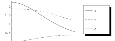
Figure 1: Plots of the matter variables $\rho$, $p$ and $E^{2}$.

ACKNOWLEDGEMENTS

SDM acknowledges that this work is based upon research supported by the South African Research Chair Initiative of the Department of Science and Technology and the National Research Foundation.

- [1] C. Wafo Soh, F.M. Mahomed, Non-static shear-free spherically symmetric charged perfect fluid distributions: a symmetry approach, Classical Quantum Gravity 17, 3063-3072, 2000.
- [2] F.M. Mahomed, A. Qadir, C. Wafo Soh, Charged spheres in general relativity revisited, Nuovo Cimento B 118, 373-381, 2003.
- [3] R. Tikekar, Exact model for a relativistic star, Journal of Mathematical Physics 31, 2454-2458, 1990.
- [4] S. D. Maharaj and P. G. L. Leach, Exact solutions for the Tikekar superdense star, Journal of Mathematical Physics 37, 430-437, 1996.
- [5] K. Komathiraj and S. D. Maharaj, Tikekar superdense stars in electric fields, Journal of Mathematical Physics 48, 042501, 2007.
- [6] R. Sharma, S. Mukherjee and S. D. Maharaj, General solution for a class of static charged spheres, General Relativity and Gravitation 33, 999-1009, 2001.
- [7] Y. K. Gupta and M. Sharma, A superdense star model as a charged analogue of Schwarzschild’s interior solution, General Relativity and Gravitation 37, 575-583, 2005.
- [8] R. Sharma, S. Kamakar and S. Mukherjee, Maximum mass of a class of cold compact stars, International Journal of Modern Physics D 15, 405-418, 2006.
- [9] R. Sharma and S. Mukherjee, Compact stars: a core envelope model, Modern Physics Letters A 38, 2535-2544, 2002.
- [10] R. Sharma and S. Mukherjee, Her X-1: a quark-diquark star?, Modern Physics Letters A 16, 1049-1059, 2001.
- [11] V. O. Thomas, B. S. Ratanpal and P. C. Vinodkumar, Core-envelope models of superdense star with anisotropic envelope, International Journal of Modern Physics D 14, 85-96, 2005.
- [12] V. O. Thomas and R. Tikekar, Relativistic fluid sphere on pseudo-spheroidal spacetime, Pramana-Journal of Physics 50, 95-103, 1998.
- [13] B. C. Paul and R. Tikekar, A core-envelope model of compact stars, Gravitation and Cosmology 11, 244-248, 2005.
- [14] S. Thirukkanesh and S. D. Maharaj, Charged anisotropic matter with a linear equation of state, Classical and Quantum Gravity 25, 235001, 2008.
- [15] M. C. Durgapal and R. Bannerji, New analytical stellar model in general relativity, Physical Review D 27, 328-331, 1983.