ARPES Spectral Function in Lightly Doped and Antiferromagnetically Ordered YBa₂Cu₃O_6+y

Abstract

At doping below $6\%$ the bilayer cuprate YBa₂Cu₃O_6+y is a collinear antiferromagnet. Independent of doping the value of the staggered magnetization at zero temperature is about $0.6\mu_{B}$. This is the maximum value of the magnetization allowed by quantum fluctuations of localized spins. In this low doping regime the compound is a normal conductor with a finite resistivity at zero temperature. These experimental observations create a unique opportunity for theory to perform a controlled calculation of the electron spectral function. In the present work we perform this calculation within the framework of the extended $t-J$ model. As one expects the Fermi surface consists of small hole pockets centered at $(\pm\pi/2,\pm\pi/2)$. The electron spectral function is very strongly anisotropic with maximum of intensity located at the inner parts of the pockets and with very small intensity at the outer parts. We also found that the antiferromagnetic correlations act against the bilayer bonding-antibonding splitting destroying it. The bilayer Fermi surface splitting is practically zero.

I Introduction

One of the central issues in the physics of cuprates is the evolution of Fermi surface upon doping. Despite a consensus on the large Fermi surface in the overdoped side, the shape and nature of the Fermi surface in underdoped cuprates remains an unresolved issue. Cuprates are doped Mott insulators. Theoretically there is no doubt that minima of the dispersion of a single hole injected in the Mott insulator are at the nodal points $(\pm\pi/2,\pm\pi/2)$. This conclusion is supported by the Angle-Resolved Photoemission Spectroscopy (ARPES) data from undoped cuprates. Damascelli03 ; Yoshida07 This implies that at a sufficiently small doping holes must go to the hole pockets. This is the small Fermi surface situation. In real compounds disorder complicates the situation and significantly masks the generic physics. For example the prototypical cuprate La_2-xSr_xCuO₄ is so disordered that holes are strongly localized at doping $x\lesssim 0.1$. In the case of strong localization the notion of the Fermi surface is ambiguous. ARPES data from underdoped La_2-xSr_xCuO₄ reveal Fermi arcs Damascelli03 ; Yoshida07 that are not consistent either with the small (hole pockets) nor with the large Fermi surface. On the other hand the very recent ARPES data from underdoped Bi₂Sr₂CaCu₂O_8+δ indicate small hole pockets. Yang

YBa₂Cu₃O_6+y (YBCO) is probably the least disordered cuprate in the low doping regime. In this paper we denote doping $x$ to be the hole concentration per unit cell of the CuO₂ layer. YBCO is not superconducting below $x\lesssim 0.06$, where the compound remains a normal conductor with delocalized holes. The zero temperature resistivity remains finite, WO01 apart of a very weak logarithmic temperature dependence sun ; doiron expected for a weak disorder. The heat conductivity also indicates delocalization of holes. sutherland05 We emphasize that this is very different from La_2-xSr_xCuO₄ where holes are localized and hence the compound is the Anderson insulator Boebinger96 ; ando02 at $x\lesssim 0.1$. com1 Ultimately, at the very low doping, $x\lesssim 0.01$, the disorder wins even in YBCO and it also becomes the Anderson insulator. WO01 It is helpful to have in mind an approximate empiric formula WO01 ; Liang

$$x\approx 0.35(y-6.20)$$ (1)

to relate the doping level $x$ and the oxygen content $y$ in underdoped YBa₂Cu₃O_6+y at $x\lesssim 0.12$. The homogeneity of YBCO is the reason why Magnetic Quantum Oscillations (MQO) were observed in this compound. Doiron-Leyraud07 ; LeBoeuf07 ; Yelland08 ; Jaudet08 ; Sebastian08 ; Audouard09 ; Sebastian09 ; Sebastian09_2 ; Singleton09 The oscillations clearly indicate small Fermi pockets, while strictly speaking nature of the pockets, including the sign of the charge of the fermion, experimentally remains a controversial issue.

The collinear antiferromagnetism (AF) in YBCO is preserved up to the doping level $x\approx 0.06$. Moreover, the zero temperature staggered magnetization $\mu\approx 0.6\mu_{B}$ is practically doping-independent, having the same value as in the parent Mott insulator. con10 This is the maximum value of magnetization allowed by quantum fluctuations of localized spins. The doping behavior of the staggered magnetization in YBCO is very different from that in La_2-xSr_xCuO₄ where the staggered magnetization decays dramatically with doping. A special mechanism has been proposed sushkov11 to explain antiferromagnetism in YBCO at $x\lesssim 0.06$. For purposes of the present work details of the mechanism are not important. The only important point is that the antiferromagnetism is independent of doping. This direct experimental observation in combination with simple metallic behaviour (finite resistivity at zero temperature that is another direct experimental observation) gives a unique opportunity to perform a controlled and fully reliable theoretical calculation of the electron spectral function at $x\lesssim 0.06$. In the present work we perform this calculation.

Our analysis is based on the $t-t^{\prime}-t^{\prime\prime}-J$ model and employs the self-consistent Born approximation (SCBA). SCBA has been widely applied to study a single hole dressed by spin fluctuations. Sushkov97 ; Kane89 ; Martinez91 ; Liu92 ; Ramsak92 ; nazarenko On the other hand application of the method at finite doping has been very limited Igarashi92 ; Kyung96 because a usual justification of the method requires a long range AF order, and the common wisdom is that even a tiny doping destroys the order. AF ordered YBCO does not comply with the common wisdom and provides a unique opportunity to address spin fluctuations up to very high accuracy. The AF order implies that the single loop vertex correction is forbidden (the ”Migdal theorem”), so SCBA is exact up to double loop corrections. Liu92

Another important property of the quasiparticle dispersion is the layer bonding-antibonding splitting in the bilayer cuprate. A density functional theory calculation shows a more or less constant splitting through out the whole Brillouin zone. Andersen95 ARPES in overdoped YBCO confirms the splitting. borisenko06 ; Fournier10 On the other hand, in the underdoped regime ARPES measurements Fournier10 indicate no such splitting. To explain this in the present paper we show that antiferromagnetic correlations between layers in the bilayer system diminish the splitting in spite of the strong chemical tendency towards the splitting. The similar result for undoped YBCO was previously obtained in Ref. nazarenko, . The antiferromagnetic correlations are due to the antiferromegnetic exchange $J_{\perp}\approx 10meV$ between the layers. Reznik96 It is worth noting that the small hole pockets are essential for the suppression of the bilayer splitting in the underdoped regime.

In the present work we consider the clean limit without any disorder. There are recent ARPES experiments on underdoped YBCO Hossain08 ; Fournier10 where the mechanism of doping is related to depositing of potassium atoms on the surface. The potassium ions give rise to a random potential for mobile holes. The degree of disorder in these experiments remains an open issue when compared with the present results.

The structure of the paper is the following. In Section II, we introduce the Hamiltonian and calculate vertexes for many-body diagrammatic technique. In Section III the method of SCBA at finite doping is discussed. The method implies the spin-charge separation. The spin-charge recombination amplitude and the ARPES spectral function is calculated in Section IV. Section V summarizes our results.

II The extended $t-J$ model for the bilayer YBCO

We simulate lightly doped YBCO by using the double layer $t-t^{\prime}-t^{\prime\prime}-J$ model with constant interlayer coupling $t_{\perp}$ and $J_{\perp}$

$$H = -t\sum_{m,\langle ij\rangle,\sigma}c_{i,m,\sigma}^{{\dagger}}c_{j,m,\sigma}-t^{\prime}\sum_{m,\langle ij\rangle^{\prime},\sigma}c_{i,m,\sigma}^{{\dagger}}c_{j,m,\sigma}$$ (2)

$$-t^{\prime\prime}\sum_{m,\langle ij\rangle^{\prime\prime},\sigma}c_{i,m,\sigma}^{{\dagger}}c_{j,m,\sigma}+J\sum_{\langle ij\rangle}{\bf S}_{i,m}\cdot{\bf S}_{j,m}$$

$$-t_{\perp}\sum_{l,\sigma}\left(c_{l,1,\sigma}^{{\dagger}}c_{l,2,\sigma}+h.c.\right)+J_{\perp}\sum_{l}{\bf S}_{l,1}\cdot{\bf S}_{l,2}$$

$$= H_{t^{\prime},t^{\prime\prime}}+H_{J,J_{\perp}}+H_{t,t_{\perp}}$$

where $t/t^{\prime}/t^{\prime\prime}$ is the nearest/next-nearest/next-next-nearest neighbor in-plane hopping, respectively, and $m=\left\{1,2\right\}$ is the plane index. Since $J_{\perp}\approx 10meV>0$, the magnetic ordering along $c-$axis is also AF. We denote the projected coordinate $\left\{i,j\right\}$ in each plane as

$$i\;\in\;\uparrow{\rm sublattice\;plane\;1}\ \ \ \equiv\ \ \ \downarrow{\rm sublattice\;plane\;2}\;$$

$$j\;\in\;\downarrow{\rm sublattice\;plane\;1}\ \ \ \equiv\ \ \ \uparrow{\rm sublattice\;plane\;2}\;$$

$$l\in\left\{i,j\right\}$$ (3)

Through out the article we set energy unit as $J=130$meV$\rightarrow 1$, hence $J_{\perp}\approx 0.08$. Schematics of the model is shown in Fig. 1.

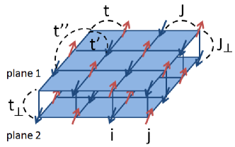
Figure 1: (color online) Schematics of double layer Hamiltonian, Eq. (2), and definition of coordinate, Eq. (3).

We use the following values of the intralayer hopping parameters $t=3.1$, $t^{\prime}=-0.5$, $t^{\prime\prime}=0.4$. While the value of $t$ corresponds to that obtained in the density functional theory calculation, Andersen95 values of $t^{\prime}=-0.5$ and $t^{\prime\prime}=0.4$ are somewhat different. Ref. Andersen95, gives for the optimally doped YBCO the following values, $t^{\prime}\approx 0.8$, $t^{\prime\prime}\approx-0.7$. Based on our results that we compare with ARPES data we believe that the values of $t^{\prime}=-0.5$ and $t^{\prime\prime}=0.4$ accepted in the present work are more suitable for underdoped YBCO. However, in the end the difference between these two sets of parameters is not qualitatively important. We take a constant interlayer tunneling $t_{\perp}$ based again on the first principle calculation, Andersen95 which shows a practically constant splitting between bonding and antibonding bands with the value of the splitting corresponding to $t_{\perp}\approx 100meV\to 1$. ARPES data from overdoped YBCO borisenko06 ; Fournier10 support this splitting. The estimate $t_{\perp}\approx 1$ is supported also by the ratio of the superexchange parameters, $0.08=J_{\perp}/J=t_{\perp}^{2}/t^{2}$.

Following the standard SCBA philosophy the Hamiltonian (2) is grouped into three sectors, $H_{t^{\prime},t^{\prime\prime}}$, $H_{J,J_{\perp}}$, and $H_{t,t_{\perp}}$, which correspond to bare hole, bare magnon, and hole-magnon interaction, respectively. We first discuss the bare magnon sector $H_{J,J_{\perp}}$. The Holstein-Primakoff bosons are defined according to sublattices in each layer, as defined in Eq. (3). In plane $1$

$$S_{i,1}^{z}=\frac{1}{2}-a_{i,1}^{{\dagger}}a_{i,1}$$

$$S_{i,1}^{+}=a_{i,1}$$

$$S_{i,1}^{-}=a_{i,1}^{{\dagger}}$$

$$S_{j,1}^{z}=-\frac{1}{2}+b_{j,1}^{{\dagger}}b_{j,1}$$

$$S_{j,1}^{+}=b_{j,1}^{{\dagger}}$$

$$S_{j,1}^{-}=b_{j,1}$$ (4)

and in plane 2

$$S_{i,2}^{z}=-\frac{1}{2}+b_{i,2}^{{\dagger}}b_{i,2}$$

$$S_{i,2}^{+}=b_{i,2}^{{\dagger}}$$

$$S_{i,2}^{-}=b_{i,2}$$

$$S_{j,2}^{z}=\frac{1}{2}-a_{j,2}^{{\dagger}}a_{j,2}$$

$$S_{j,2}^{+}=a_{j,2}$$

$$S_{j,2}^{-}=a_{j,2}^{{\dagger}}\ .$$ (5)

The Fourier transform is

$$a_{i,1}=\sqrt{\frac{2}{N}}\sum_{\bf q}a_{{\bf q},1}e^{i{\bf q\cdot r}_{i}}$$

$$b_{j,1}=\sqrt{\frac{2}{N}}\sum_{\bf q}b_{{\bf q},1}e^{i{\bf q\cdot r}_{j}}$$

$$a_{j,2}=\sqrt{\frac{2}{N}}\sum_{\bf q}a_{{\bf q},2}e^{i{\bf q\cdot r}_{j}}$$

$$b_{i,2}=\sqrt{\frac{2}{N}}\sum_{\bf q}b_{{\bf q},2}e^{i{\bf q\cdot r}_{i}}\ ,$$ (6)

where summation over ${\bm{q}}$ is restricted inside Magnetic Brillouin Zone (MBZ). By introducing parity $+$ and $-$ bases with respect to interchange of two planes

$$a_{{\bf q},\pm}=\frac{1}{\sqrt{2}}\left(a_{{\bf q},1}\pm a_{{\bf q},2}\right)$$

$$b_{{\bf q},\pm}=\frac{1}{\sqrt{2}}\left(b_{{\bf q},1}\pm b_{{\bf q},2}\right)$$ (7)

and Bogoliubov transformation

$$a_{{\bf q},\pm}=u_{{\bf q},\pm}\alpha_{{\bf q},\pm}+v_{{\bf q},\pm}\beta_{{\bf-q},\pm}^{{\dagger}}$$

$$b_{{\bf-q},\pm}=v_{{\bf q},\pm}\alpha_{{\bf q},\pm}^{{\dagger}}+u_{{\bf q},\pm}\beta_{{\bf-q},\pm}$$ (8)

one can diagonalize the HamiltonianTranquada89 ; Reznik96

$$H_{J,J_{\perp}} = \sum_{\bf q}\left(\alpha_{{\bf q},+}^{{\dagger}}\alpha_{{\bf q},+}+\beta_{{\bf q},+}^{{\dagger}}\beta_{{\bf q},+}\right)\omega_{{\bf q},+}$$

$$+ \sum_{\bf q}\left(\alpha_{{\bf q},-}^{{\dagger}}\alpha_{{\bf q},-}+\beta_{{\bf q},-}^{{\dagger}}\beta_{{\bf q},-}\right)\omega_{{\bf q},-}\;,$$

$$\omega_{{\bf q},\pm} = 2J\left\{(1+\frac{\alpha_{\perp}}{4})^{2}-(\gamma_{\bf q}\pm\frac{\alpha_{\perp}}{4})^{2}\right\}^{1/2}$$

$$\gamma_{\bf q} = \frac{1}{2}\left(\cos q_{x}+\cos q_{y}\right)\ ,$$ (9)

where we denote $\alpha_{\perp}=J_{\perp}/J$. Here $\omega_{\bf q,+}$ mode is gapless at $(0,0)$ and gapped at $(\pi,\pi)$, while $\omega_{\bf q,-}$ mode is the opposite. This is consistent with the fact that optical mode is frequently referred to even parity, and acoustic mode to odd parity in inelastic neutron scattering experiments which practically measure magnon dispersion near $(\pi,\pi)$.Tranquada89 ; Reznik96 The Bogoliubov coefficients are

$$u_{{\bf q},\pm}=\sqrt{\frac{J+\frac{J_{\perp}}{4}}{\omega_{{\bf q},\pm}}+\frac{1}{2}}$$

$$v_{{\bf q},\pm}=-{\rm sign}({\gamma_{\bf q}\pm\frac{\alpha_{\perp}}{4}})\sqrt{\frac{J+\frac{J_{\perp}}{4}}{\omega_{{\bf q},\pm}}-\frac{1}{2}}$$ (10)

The magnon Green’s function is defined as

$$D_{\pm}(\omega,{\bf q}) = -i\int_{0}^{\infty}\langle T\alpha_{\bf q,\pm}(t)\alpha_{\bf q,\pm}^{{\dagger}}(0)\rangle e^{i\omega t}dt$$ (11)

$$= -i\int_{0}^{\infty}\langle T\beta_{\bf q,\pm}(t)\beta_{\bf q,\pm}^{{\dagger}}(0)\rangle e^{i\omega t}dt$$

$$= \frac{1}{\omega-\omega_{\bf q,\pm}+i\eta}\;.$$

In the present work we do not consider renormalization of magnon dispersion due to interaction with holes, but simply adopt the magnon sector of undoped Mott insulator. This assumption is justified because $\mu$SR measurements indicate almost unrenormalized staggered magnetization up to doping level $x\approx 0.06$.con10 The magnon dispersion close to the Goldstone point ${\bf q}=0$ [equivalent to ${\bf q}=(\pm\pi,\pm\pi)$] is somewhat changed under doping. sushkov11 However, due to the Adler’s theorem, magnons close to the Goldstone point practically do not influence the hole dispersion, see discussion below. The main contribution to the hole dispersion comes from magnons that are far away from the Goldstone point. For this regime, resonant inelastic X-ray scattering(RIXS) clearly demonstrates that magnons are almost independent of doping. RIX Theoretical analysis of the RIXS experimental data is an important problem that will be considered elsewhere. wchen11

To address the bare hole dispersion from the $H_{t^{\prime},t^{\prime\prime}}$ term, we first define hole operators according to the coordinate in Eq. (3)

$$d_{{\bf k},1,\uparrow}=\sqrt{\frac{2}{N(1/2+m)}}\sum_{j}c_{j,1,\downarrow}^{{\dagger}}e^{-i{\bf k\cdot r}_{j}}$$

$$d_{{\bf k},1,\downarrow}=\sqrt{\frac{2}{N(1/2+m)}}\sum_{i}c_{i,1,\uparrow}^{{\dagger}}e^{-i{\bf k\cdot r}_{i}}$$

$$d_{{\bf k},2,\uparrow}=\sqrt{\frac{2}{N(1/2+m)}}\sum_{i}c_{i,2,\downarrow}^{{\dagger}}e^{-i{\bf k\cdot r}_{i}}$$

$$d_{{\bf k},2,\downarrow}=\sqrt{\frac{2}{N(1/2+m)}}\sum_{j}c_{j,2,\uparrow}^{{\dagger}}e^{-i{\bf k\cdot r}_{j}}\ ,$$ (12)

where $m=|\langle S_{z}\rangle|\approx 0.3$, see Ref. Sushkov97, . The fixed parity states are

$$d_{{\bf k},\pm,\sigma}=\frac{1}{\sqrt{2}}\left(d_{{\bf k},1,\sigma}\pm d_{{\bf k},2,\sigma}\right)$$ (13)

The bare hole dispersion is then

$$H_{t^{\prime},t^{\prime\prime}}=\sum_{{\bf k},\sigma}\epsilon_{{\bf k},+}^{0}d_{{\bf k},+,\sigma}^{{\dagger}}d_{{\bf k},+,\sigma}+\sum_{{\bf k},\sigma}\epsilon_{{\bf k},-}^{0}d_{{\bf k},-,\sigma}^{{\dagger}}d_{{\bf k},-,\sigma}$$

$$\epsilon_{{\bf k},\pm}^{0}=\epsilon_{{\bf k}}^{0}=4t^{\prime}\cos k_{x}\cos k_{y}+2t^{\prime\prime}\left(\cos 2k_{x}+\cos 2k_{y}\right)$$

Since site $i$ on plane $1$ and site $i$ on plane $2$ belong to different sublattices, the interlayer hopping does not enter the bare dispersion. This is the reason why the AF correlations suppress the interlayer hopping. Similar to the in-plane nearest-neighbor hopping, the interlayer hopping contains the spin-flip process that contributes to the hole-magnon interaction. The corresponding vertex therefore contains contributions from both $t$ and $t_{\perp}$, as calculated in Appendix A. The Hamiltonian $H_{t,t_{\perp}}$ and the corresponding vertex read

$$H_{t,t_{\perp}}=\sum_{{\bf k,q},\gamma\delta\nu}g_{{\bf k,q},\gamma\delta}\left(d_{{\bf k+q},\nu,\downarrow}^{{\dagger}}d_{{\bf k},\delta,\uparrow}\alpha_{{\bf q},\gamma}\right.$$

$$\;\;\;\;\;\;\;\;\;\;\;\left.+d_{{\bf k+q},\nu,\uparrow}^{{\dagger}}d_{{\bf k},\delta,\downarrow}\beta_{{\bf q},\gamma}\right)+h.c.\;,$$

$$g_{{\bf k,q},\gamma\delta}=\frac{4t}{\sqrt{N}}\left(\gamma_{\bf k}u_{{\bf q},\gamma}+\gamma_{\bf k+q}v_{{\bf q},\gamma}\right)$$

$$\;\;\;\;\;\;\;+\delta\frac{t_{\perp}}{\sqrt{N}}\left(u_{{\bf q},\gamma}+\gamma v_{{\bf q},\gamma}\right)\;.$$ (15)

We denote the parity index by $\gamma,\delta,\nu=\pm 1$. This is the parity of the annihilated magnon, the annihilated hole, and the created hole, as shown in Fig. 2(a). Conservation of parity implies $\nu=\gamma\delta$. The vertex (15) is zero at $q=0$, this is a consequence of Adler’s theorem, and this is why the contribution of magnons with small momenta to the self-energy is negligible.

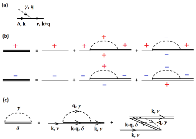
Figure 2: (color online) Feynman diagrams for (a) the hole-magnon vertex defined in Eq. (15), (b) Dyson’s equation Eq. (19) for $G_{d\pm}$, and (c) schematics of advanced and retarded part of each self-energy diagram, as calculated in Eq. (37).

III Self Consistent Born Approximation

The SCBA is based on summation of diagrams having the highest possible power of the hopping parameter $t$ at a given number of loops. Sushkov97 ; Kane89 ; Martinez91 ; Liu92 ; Ramsak92 ; nazarenko This implies that the method is justified at $t/J>1$. A very important point is that due to the spin structure of the theory (conservation of $S_{z}$) there is no single loop correction to the hole-magnon vertex shown in Fig. 2(a). Therefore, the diagrams having the highest possible power of $t$ are the rainbow diagrams. Thus, SCBA is summation of rainbow diagrams. Again, the method is justified due to (i) absence of the single loop vertex correction, (ii) due to $t/J>1$.

Compared to the single hole in a single layer case, Sushkov97 ; Kane89 ; Martinez91 ; Liu92 ; Ramsak92 the present calculation has two complications: the double layer and the finite doping. Importantly, since we consider the collinear AF state, the both points (i) and (ii) justifying the method are still valid in spite of the complications. We stress that although the finite doping case has been discussed before, Igarashi92 ; Kyung96 it is not until current calculation that SCBA is rigorously formulated for a real material that AF order persists at finite doping.

At finite doping we have to use the Feynman Green’s function of the hole

$$G_{d\sigma\pm}(\epsilon,{\bf k})=-i\int_{-\infty}^{\infty}\langle Td_{{\bf k},\pm,\sigma}(t)d_{{\bf k},\pm,\sigma}^{{\dagger}}(0)\rangle e^{i\epsilon t}dt$$ (16)

instead of the retarded Green’s function in the undoped case. Sushkov97 ; Kane89 ; Martinez91 ; Liu92 ; Ramsak92 ; nazarenko The Green’s function (16) has the parity index $\pm$ reflecting the double layer structure, and the pseudospin index $\sigma=\uparrow\downarrow$ reflecting the AF structure. Since the up and down pseudospins are degenerate, we omit the psedospin index $\sigma$ for the rest of the article, although one should keep in mind that vertexes in Eq. (15) always flip the pseudospin. In the calculation of self-energy, we adopt the spectral representation

$$G_{d\pm}(\epsilon,{\bf k}) = \int_{0}^{\infty}dx\frac{A_{\pm}(x,{\bf k})}{\epsilon-x+i0}+\int_{-\infty}^{0}dx\frac{B_{\pm}(x,{\bf k})}{\epsilon-x-i0}\;.$$ (17)

The chemical potential is set equal to zero. The technical advantage of using spectral representation is that it ensures the causality of Dyson’s equation in any order, as we calculate the self-energy in terms of the spectral functions. This is important because Dyson’s equation typically converges at about $10\sim 20$th order, therefore causality must be ensured at each order. The doping is

$$2x=2\sum_{\bf k}\sum_{\pm}\int_{-\infty}^{0}dxB_{\pm}(x,{\bf k})\ .$$ (18)

The summation over ${\bf k}$ is limited inside the MBZ. The coefficient $2$ in the left-hand-side of (18) is due to the bilayer, the coefficient $2$ in the right-hand-side is due to pseudospin.

Dyson’s equations shown schematically in Fig. 2(b) read

$$G_{d+}(\epsilon,{\bf k})=\left[\epsilon-\epsilon_{\bf k,}^{0}-\Sigma_{++}(\epsilon,{\bf k})-\Sigma_{--}(\epsilon,{\bf k})+i0\right]^{-1}$$

$$G_{d-}(\epsilon,{\bf k})=\left[\epsilon-\epsilon_{\bf k,}^{0}-\Sigma_{+-}(\epsilon,{\bf k})-\Sigma_{-+}(\epsilon,{\bf k})+i0\right]^{-1}$$

(19)

The subscripts in the self-energy $\Sigma_{\pm,\pm}$ indicate parities of the intermediate hole and magnon as it is shown in Fig. 2(b). Note that the considered theory does not possess the usual cross-leg-symmetry of vertexes. Therefore the usual Feynman technique is not sufficient, Kyung96 and one has to adopt the Goldstone-Brueckner technique that explicitly separates forward in time and backward in time diagrams, as shown in 2(c). Explicit expressions for the self-energy are derived in Appendix B and presented in Eq. (37).

We now discuss symmetry properties of Green’s functions imposed by definitions of operators (7) and (13). Due to the chequerboard AF order, hole and magnon operators change parity under translation by the AF wave vector ${\bf Q}=(\pi,\pi)$, ${\bf k}\rightarrow{\bf k+Q}$.

$$d_{{\bf k},+,\uparrow}=-d_{{\bf k+Q},-,\uparrow}$$

$$d_{{\bf k},+,\downarrow}=d_{{\bf k+Q},-,\downarrow}$$

$$\alpha_{{\bf q},+}=\alpha_{{\bf q},-}$$

$$\beta_{{\bf q},+}=-\beta_{{\bf q},-}\ .$$ (20)

Hence the Green’s functions satisfy the following symmetry relations

$$G_{d+}(\epsilon,{\bf k+Q})=G_{d-}(\epsilon,{\bf k})\;,$$

$$D_{+}(\omega,{\bf q+Q})=D_{-}(\omega,{\bf q})\;.$$ (21)

As a result, the hole dispersion of parity $+$ and $-$ swap at the MBZ boundary, as previously reported for the single hole case. nazarenko This implies that at the MBZ boundary, the magnon dispersion of either parity are degenerate, and the hole dispersion of either parity are also degenerate, as addressed below.

Figure 3: Spectral functions $S_{d+}$ (a) and $S_{d-}$ (b) for different values of ${\bf k}$ along the nodal direction from $(0,0)$ to $(\pi,\pi)$. There is an offset 0.2 between subsequent values of ${\bf k}$. The doping level is $x=0.059$.

Iterative numerical solution of Eqs. (19),(37) requires more computational power compared to solution of similar equations for undoped single layer case. Sushkov97 ; Kane89 ; Martinez91 ; Liu92 ; Ramsak92 ; nazarenko Nevertheless the solution is straightforward. We solve Eq. (19) inside MBZ on a $64\times 64$ cluster, with about 1700 frequency points (the frequency grid is $\Delta\omega=0.015$). We present plots of the hole spectral function $S_{d}$ defined as $A(\epsilon,{\bm{k}})$ if $\epsilon>0$ and as $B(\epsilon,{\bm{k}})$ if $\epsilon<0$, see Eq. (17).

$$S_{d\pm}(\epsilon,{\bm{k}})=A_{\pm}(\epsilon,{\bm{k}})+B_{\pm}(\epsilon,{\bm{k}})\ .$$ (22)

Figs. 3(a) and (b) display the hole spectral functions (offset 0.2) of positive and negative parities for doping level $x=0.059$. This doping is close to the highest doping level at which AF order persists while superconductivity has yet taken place. con10 To show more details the spectral function $S_{d+}$ is plotted in Fig. 4 for ${\bf k}=(0,0)$, ${\bf k}=(\pi/2,\pi/2)$ and ${\bf k}=(\pi,0)$.

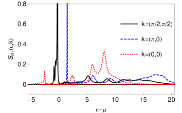
Figure 4: Spectral functions $S_{d+}$ for ${\bf k}=(0,0)$, ${\bf k}=(\pi/2,\pi/2)$ and ${\bf k}=(\pi,0)$. The doping level is $x=0.059$.

The spectral functions show a striking similarity to the hole spectral function in an undoped insulator: there is a well defined quasiparticle peak at low energy, and a large incoherent part at higher energy. In addition, a small but significant incoherent part is observed at energy below the quasiparticle peak, due to the electron plus multiple magnon configurations in the emission channel. Along nodal direction, the quasiparticle peak is most pronounced near $(\pi/2,\pi/2)$, and gradually decreases as approaching $(0,0)$ and $(\pi,\pi)$ where it is dissolved in the hole-magnon continuum.

The position of the quasiparticle peak determines the quasiparticle dispersion $\epsilon_{\bf k}$. The dispersion is shown in Fig. 5(a) along a certain line in the Brillouin Zone (BZ).

Figure 5: (a) The quasiparticle dispersion, and (b) the quasiparticle residue $Z_{d}$ along a certain line in BZ. The doping level is $x=0.059$.

Formation of small Fermi surface with hole pockets at ${\bf k}=(\pi/2,\pi/2)$ is evident. Eq. (20), imposes a nontrivial constraint on the dispersion: From ${\bf k}=(0,0)$ to $(\pi,\pi)$, one sees that the two parity bands are symmetric but swap at the MBZ boundary ${\bf k}=(\pi/2,\pi/2)$. Along the MBZ boundary, as shown in the section from ${\bf k}=(\pi,0)$ to $(\pi/2,\pi/2)$, the two bands are degenerate. At the Fermi surface $\epsilon_{{\bf k}+}$ differs from $\epsilon_{{\bf k}-}$ by only $\approx 25$meV. We remind that for the value $t_{\perp}=J=130$meV used in the calculation, one expects the splitting to be $260$meV. Therefore AF correlations strongly suppress the bilayer splitting.

In the section of $(\pi,\pi)$ to $(\pi,0)$ in Fig. 5(a), one sees a local dispersion minimum near $(\pi,\pi/2)$. However, in the $(\pi/2,\pi/2)$ to $(\pi,\pi/2)$ section, ones sees that $(\pi,\pi/2)$ is a local maximum. Hence, there is a saddle point near $(\pi,\pi/2)$, or equivalently near $(0,\pi/2)$, $(\pi/2,0)$. The saddle point gives a very large contribution to the density of states, $N_{\pm}(\epsilon)=\int\left[A_{\pm}(\epsilon,{\bf k})+B_{\pm}(\epsilon,{\bf k})\right]d^{2}{\bf k}/(2\pi)^{2}$. Due to the saddle point the electron response function is very strongly peaked at ${\bf q}\approx(\pi/2,0)$, $\omega\approx 100$meV. Interestingly, these parameters are very close to where the anomaly in the breathing phonon mode is observed. phonon Although further investigation is necessary to clarify this point, we anticipate that the saddle point plays a crucial role in the anomaly.

The quasiparticle residue $Z_{d\bf k\pm}$ is shown in Fig. 5(b) along the same line in BZ as dispersion. Along the nodal direction, the quasiparticle residue $Z_{d\bf k\pm}$ is maximum at the bottom of the pocket, and decreases smoothly as moving away from the pocket. This smooth dependence is very similar to the residue in undoped parent compound. Sushkov97 Since the pocket is rather small, the residue inside the pocket can be well approximated by a constant $Z_{d\bf k\pm}\approx 0.34$. The bottom of the pocket is well fitted by a parabolic band $\epsilon_{\bf k\pm}\approx\beta_{1}k_{1}^{2}/2+\beta_{2}k_{2}^{2}/2$, where $\beta_{1}$ and $\beta_{2}$ represent the inverse effective mass along and orthogonal to the nodal direction, respectively. At the highest doping examined, $x=0.059$, we obtain $\beta_{1}\approx 3.4$, $\beta_{2}\approx 1.8$, which yields the anisotropy $\beta_{1}/\beta_{2}\approx 1.9$. The value of the effective mass $m^{\ast}=1/\sqrt{\beta_{1}\beta_{2}}$ converted to conventional units is $m^{\ast}\approx 1.6m_{e}$. This value is consistent with the mass measured in MQO. Doiron-Leyraud07 ; LeBoeuf07 ; Yelland08 ; Jaudet08 ; Sebastian08 ; Audouard09 ; Sebastian09 ; Sebastian09_2 ; Singleton09

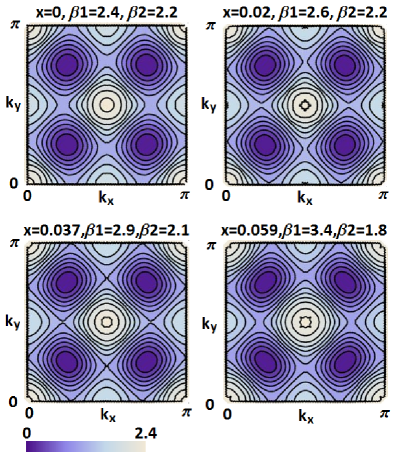
Figure 6: (color online) Maps of the parity average dispersion $\epsilon_{\bf k}=(\epsilon_{\bf k,+}+\epsilon_{\bf k,-})/2$ at different doping levels. Effective mass along ($\beta_{1}$) and orthogonal ($\beta_{2}$) to the nodal direction is calculated by fitting the bottom of the pocket with $\epsilon_{\bf k}\approx\beta_{1}k_{1}^{2}/2+\beta_{2}k_{2}^{2}/2$. The ellipticity of hole pockets, represented by $\sqrt{\beta_{1}/\beta_{2}}$, increases with doping indicating a deviation from the rigid band approximation.

Maps of the parity average dispersion, $\epsilon_{\bf k}=(\epsilon_{\bf k,+}+\epsilon_{\bf k,-})/2$, are shown in Fig. 6 for four values of doping. The total bandwidth $\approx 2.4J\approx 0.3$eV remains roughly the same independent of doping. This bandwidth is very close to the value indicated by ARPES in undoped single layer compound. Wells95 ; LaRosa97 By comparing different doping levels in Fig. 6, it is also clear that the ellipticity of the pocket increases with doping. More precisely, $\beta_{1}$ is increasing while $\beta_{2}$ is decreasing at higher doping. Enhancement of ellipticity with doping is consistent with a previous analytical calculation. Kotov04 The doping dependent ellipticity implies that the rigid band approximation is strictly speaking not valid. However, the change of ellipticity, although being significant, is not dramatic, so the rigid band approximation is fairly reasonable. Moreover, the average effective mass $m^{\ast}=1/\sqrt{\beta_{1}\beta_{2}}$ is roughly doping independent.

The present approach certainly supports the small Fermi surface Luttinger’s theorem. The doping calculated according to Eq. (18) coincides with the area of the small Fermi surface. It is worth noting that numerically this coincidence is quite nontrivial, the negative energy incoherent part of the Green’s function is absolutely significant for this.

IV Spin-charge recombination and ARPES spectral function

In the SCBA approach spin and charge are separated, there are nonitinerant spins and there are itinerant spinless holes. The hole has a pseudospin indicating a chequerboard magnetic sublattice, but the pseudospin is different from usual spin. In ARPES process spin and charge recombine to physical electrons. To calculate the recombination amplitude we follow the approach of Ref. Sushkov97, modifying the approach to the bilayer case and to finite doping. ARPES measures electrons with true spin, regardless which sublattice the electron comes from. The annihilation operator of an electron from $m$-th plane ($m=1,2$) is

$$c_{{\bf k},m,\sigma}=\sqrt{\frac{2}{N}}\sum_{l\in\left\{i,j\right\}}c_{l,m,\sigma}e^{-i{\bf k\cdot r}_{l}}\;,$$ (23)

where $\sigma$ is the true spin. Notice that the definition (23) is properly normalized, because

$$\langle 0|c_{{\bf k},1,\uparrow}^{{\dagger}}c_{{\bf k},1,\uparrow}|0\rangle=\frac{2}{N}\langle 0|\sum_{l\in\left\{i,j\right\}}c_{l,1,\uparrow}^{{\dagger}}c_{l,1,\uparrow}|0\rangle$$

$$\;\;\;=\frac{2}{N}\langle 0|\sum_{l\in\left\{i,j\right\}}\left(\frac{1}{2}+S_{l}^{1z}\right)|0\rangle=1\;.$$ (24)

To establish the connection with hole operators in Eq. (13), one needs to rotate electron operators into the fixed parity basis

$$c_{{\bf k},\pm,\sigma}=\frac{1}{\sqrt{2}}\left(c_{{\bf k},1,\sigma}\pm c_{{\bf k},2,\sigma}\right)$$ (25)

The connection between electron and hole Green’s function is then associated with the following vertices Sushkov97 ; Brink98

$$a_{\bf k} = \langle 0|d_{{\bf-k},+,\uparrow}c_{{\bf k},+,\downarrow}|0\rangle$$

$$= \langle 0|d_{{\bf-k},-,\uparrow}c_{{\bf k},-,\downarrow}|0\rangle=\sqrt{1/2+m}\;,$$

$$b_{{\bf k,q},+} = \langle 0|\beta_{\bf q,+}d_{{\bf-k-q},+,\downarrow}c_{{\bf k},+,\downarrow}|0\rangle$$

$$= \langle 0|\beta_{\bf q,+}d_{{\bf-k-q},-,\downarrow}c_{{\bf k},-,\downarrow}|0\rangle=\sqrt{\frac{1}{N}}v_{\bf q,+}$$

$$b_{{\bf k,q},-} = \langle 0|\beta_{\bf q,-}d_{{\bf-k-q},+,\downarrow}c_{{\bf k},-,\downarrow}|0\rangle$$

$$= \langle 0|\beta_{\bf q,-}d_{{\bf-k-q},-,\downarrow}c_{{\bf k},+,\downarrow}|0\rangle=\sqrt{\frac{1}{N}}v_{\bf q,-}$$

$$c_{{\bf k,q},+} = \langle 0|d_{{\bf-k+q},+,\downarrow}c_{{\bf k},+,\downarrow}\alpha_{\bf q,+}^{{\dagger}}|0\rangle$$

$$= \langle 0|d_{{\bf-k+q},-,\downarrow}c_{{\bf k},-,\downarrow}\alpha_{\bf q,+}^{{\dagger}}|0\rangle=\sqrt{\frac{1}{N}}u_{\bf q,+}$$

$$c_{{\bf k,q},-} = \langle 0|d_{{\bf-k+q},+,\downarrow}c_{{\bf k},-,\downarrow}\alpha_{\bf q,-}^{{\dagger}}|0\rangle$$ (26)

$$= \langle 0|d_{{\bf-k+q},-,\downarrow}c_{{\bf k},+,\downarrow}\alpha_{\bf q,-}^{{\dagger}}|0\rangle=\sqrt{\frac{1}{N}}u_{\bf q,-}$$

Here $|0\rangle$ is the ground state of the doped system. The vertex $a_{\bf k}$ describes the process of instant creation of an electron with momentum ${\bf k}$ and a hole with momentum $-{\bf k}$, $|0\rangle\to c_{{\bf k},+,\downarrow}^{{\dagger}}d_{{\bf-k},+,\uparrow}^{{\dagger}}|0\rangle$, as it is shown in Fig. 7(a).

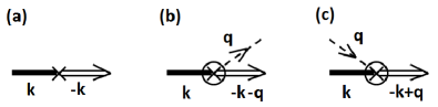
Figure 7: Vertices involved in the photoemission process, as defined in Eq. (26)

In the figure electron is shown by the bold solid line moving from the left, and the hole is shown by the double line. The direction of the electron line in Fig. 7 strictly speaking is not correct, as the electron has to appear in the final state only. Nevertheless, in figures we always show electron in the initial state just for a convenient graphical presentation. This way of presentation does not cause any problems since we always have only one electron. The vertex $b_{{\bf k,q},\gamma}$ describes the process of instant creation of an electron with momentum ${\bf k}$, a hole with momentum $-{\bf k}-{\bf q}$ and a magnon with momentum ${\bf q}$, as shown in Fig. 7(b). We define the parity index $\gamma$ to be parity of the magnon. The vertex $c_{{\bf k,q},\gamma}$ describes the process of annihilation of a magnon with momentum ${\bf q}$ and instant creation of an electron with momentum ${\bf k}$ and a hole with momentum $-{\bf k}+{\bf q}$, as shown in Fig. 7(c). Derivation of the vertices (26) is presented in Appendix A. The analysis of ARPES in undoped parent compound at zero temperature requires only $a_{\bf k}$ and $b_{{\bf k,q}}$ vertices, Sushkov97 whereas the undoped compound at nonzero temperatures requires additional vertex $c_{\bf k,q}$, Brink98 because there are thermally excited magnons in the initial state. Presently we consider a doped compound at zero temperature, so there are no thermally excited magnetic fluctuations, but there are additional magnetic fluctuations due to doping. Thus all three vertices are involved in the present calculation.

The electron Green’s function is defined in the standard way.

$$G_{c\sigma\pm}(\epsilon,{\bf k})=-i\int_{-\infty}^{\infty}\langle Tc_{{\bf k},\pm,\sigma}^{{\dagger}}(t)c_{{\bf k},\pm,\sigma}(0)\rangle e^{i\epsilon t}dt$$ (27)

Here $\sigma$ is the true spin index. Notice that the two spins are degenerate, so below we omit the spin index in $G_{c\pm}$. Dyson equations relating $G_{c}$ and already calculated $G_{d}$ are similar to that derived in Refs. Sushkov97, ; Brink98, . The equations are shown graphically in Fig. 8 and presented below in analytical form

$$G_{c+}(\epsilon,{\bf k}) = a_{\bf k}^{2}G_{d+}(\epsilon,{\bf-k})+\Sigma_{++}^{(1)}(\epsilon,{\bf k})+\Sigma_{--}^{(1)}(\epsilon,{\bf k})$$

$$+ 2a_{\bf k}G_{d+}(\epsilon,{\bf-k})\left[\Sigma_{++}^{(2)}(\epsilon,{\bf k})+\Sigma_{--}^{(2)}(\epsilon,{\bf k})\right]$$

$$+ G_{d+}(\epsilon,{\bf-k})\left[\Sigma_{++}^{(2)}(\epsilon,{\bf k})+\Sigma_{--}^{(2)}(\epsilon,{\bf k})\right]^{2}$$

$$G_{c-}(\epsilon,{\bf k}) = a_{\bf k}^{2}G_{d-}(\epsilon,{\bf-k})+\Sigma_{+-}^{(1)}(\epsilon,{\bf k})+\Sigma_{-+}^{(1)}(\epsilon,{\bf k})$$ (28)

$$+ 2a_{\bf k}G_{d-}(\epsilon,{\bf-k})\left[\Sigma_{+-}^{(2)}(\epsilon,{\bf k})+\Sigma_{-+}^{(2)}(\epsilon,{\bf k})\right]$$

$$+ G_{d-}(\epsilon,{\bf-k})\left[\Sigma_{+-}^{(2)}(\epsilon,{\bf k})+\Sigma_{-+}^{(2)}(\epsilon,{\bf k})\right]^{2}$$

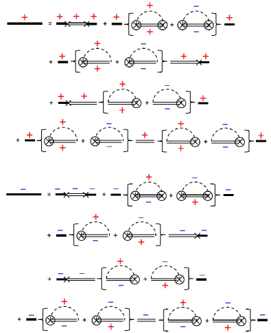
Figure 8: (color online) Dyson’s equations relating $G_{c\pm}$ and $G_{d\pm}$. The thick line represents $G_{c\pm}$, and the double line represents $G_{d\pm}$.

We emphasize that the conventional self-energy $\Sigma_{\gamma\delta}$ appears only in Dyson’s equation (19) for $G_{d}$. Equations (28) contain different kinds of self-energy. The self-energy $\Sigma^{(1)}_{\gamma\delta}$ has two vertices $b_{{\bf k,q},\gamma}$ or $c_{{\bf k,q},\gamma}$ denoted by the crossed circle. The self-energy $\Sigma^{(2)}_{\gamma\delta}$ has only one vertex $b_{{\bf k,q},\gamma}$ or $c_{{\bf k,q},\gamma}$ denoted by the crossed circle and one vertex $g_{\bf k,q}$ (see Eq. (15)) shown by a simple attachment of the dashed line (magnon) to the double line (hole). The subscript $\{\gamma\delta\}$ in the self-energies shows parities of the intermediate magnon and hole, respectively, as displayed in Fig. 8. Expressions for $\Sigma_{\gamma\delta}^{(1)}$ and $\Sigma_{\gamma\delta}^{(2)}$ are presented in Appendix B.

Figure 9: Spectral functions $S_{c+}$ (a) and $S_{c-}$ (b) for different values of ${\bf k}$ along the nodal direction from $(0,0)$ to $(\pi,\pi)$. There is an offset 0.2 between subsequent values of ${\bf k}$. The doping level is $x=0.059$.

It is worth noting that meaning of Dyson’s equations, Eq. (28) is different from that of Eq. (19). Eq. (19) is a real dynamic equation for $G_{d\pm}$, which requires an iterative solution. On the other hand, Eq. (28) is just a relation between $G_{c\pm}$ and $G_{d\pm}$ that describes the spin-charge recombination in the photoemission process. Once $G_{d\pm}$ is known, we calculate the right hand side in Eq. (28) and $G_{c\pm}$ is determined. The Greens’s function $G_{c\pm}$ has the spectral representation similar to Eq. (17) and a spectral function similar to Eq. (22). The spectral functions $S_{c\pm}$ for $x=0.059$ are displayed in Fig. 9(a) and Fig. 9(b). The position of the quasiparticle peak is exactly the same as that in $G_{d\pm}$, as one expects from general considerations and it is also evident from Eqs. (28). However, the quasiparticle residue of $G_{c\pm}$, denoted by $Z_{c\pm}$, is very different from that of $G_{d\pm}$. Since $G_{c\pm}$ represents electrons of either sublattice, there is no a Bloch theorem to require $Z_{c\pm}$ to be symmetric with respect to MBZ boundary.

In fact, our calculation shows a very asymmetric $Z_{c\pm}$, as shown in Fig. 10 along a certain line in BZ. Along the nodal direction, $Z_{c\pm}$ first increases from ${\bf k}=(0,0)$ to the inner edge(red dotted vertical line) of the Fermi pocket. After that $Z_{c\pm}$ drops abruptly as ${\bf k}$ goes across the pocket inside the Fermi surface (although this part of the Green’s function is not measurable by ARPES). A less steep drop of $Z_{c\pm}$ takes place from the outer edge (blue dotted vertical line) of the pocket to the point ${\bf k}=(\pi,\pi)$. The difference between $Z_{c\pm}$ on the inner side of the pocket and the outer side is very significant.

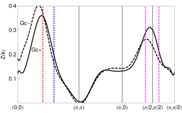
Figure 10: (color online) The quasiparticle residue $S_{c}$ along the same line as in Fig. 5. Doping level is $x=0.059$. Vertical dashed lines show Fermi points.

The above analysis is performed within the double layer $t-t^{\prime}-t^{\prime\prime}-J$ model. The $t-t^{\prime}-t^{\prime\prime}-J$ model can originate from the single band Hubbard model or from a multi-band Hubbard model. The origin of the $t-t^{\prime}-t^{\prime\prime}-J$ model is not important for the dynamic equation (19). However, the origin is important for the spin-charge recombination amplitude given by Eq. (28). Depending on the original model, there is an additional significant contribution to the asymmetry of the electron spectral function between inside and outside of MBZ. Analysis performed in Ref. Sushkov97, shows that in the case of the single band Hubbard model the vertices in Eq. (26) should be modified by

$$a_{\bf k}\rightarrow a_{\bf k}\left(1+\frac{J}{t}\gamma_{\bf k}\right)$$

$$b_{{\bf k,q},\pm}\rightarrow b_{{\bf k,q},\pm}\left(1+\frac{J}{t}\gamma_{\bf k}\right)$$

$$c_{{\bf k,q},\pm}\rightarrow c_{{\bf k,q},\pm}\left(1+\frac{J}{t}\gamma_{\bf k}\right)$$ (29)

which effectively modify quasiparticle residue $Z_{c\pm}$ by

$$Z_{c\pm}\to Z_{c\pm}^{H}=Z_{c\pm}\left(1+\frac{J}{t}\gamma_{\bf k}\right)\;.$$ (30)

Following Ref. Sushkov97, we call this correction the Hubbard model correction. Plots of the parity-averaged quasiparticle residue, $\left[Z_{c+}^{H}({\bf k})+Z_{c-}^{H}({\bf k})\right]/2$, along the nodal direction are presented in Fig. 11 for three different values of doping. In the same figure, we also present colour maps of the following function

$$\overline{Z}_{c}^{H}({\bf k})=\frac{\delta^{2}}{2}\left\{\frac{Z_{c+}^{H}(\bf k)}{(\epsilon_{\bf k,+}-\mu)^{2}+\delta^{2}}+\frac{Z_{c-}^{H}(\bf k)}{(\epsilon_{\bf k,-}-\mu)^{2}+\delta^{2}}\right\}\;$$ (31)

This formula gives a way to image the quasiparticle residue at the Fermi surface. The broadening $\delta$ can be taken as a result of disorder and/or experimental resolution, or purely for the sake of imaging. We choose $\delta=0.1$, which corresponds to the halfwidth $\Gamma=2\delta=26$meV.

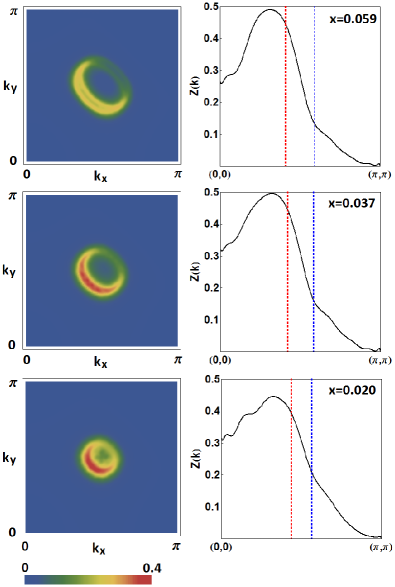
Figure 11: (color online) Right column: The parity average residue $\left[Z_{c+}^{H}({\bf k})+Z_{c-}^{H}({\bf k})\right]/2$ of the electron Green’s function along the nodal direction. Vertical dashed lines show Fermi points. The ARPES intensity is proportional to the residue outside the Fermi surface. Left column: colour maps of the ARPES intensity at the Fermi surface. The plots are presented for three values of doping, $x=0.02,0.037,0.059$.

From the right column of Fig. 11 we observe that at the largest doping examined, $x=0.059$, the ARPES intensity in the inner side (red dotted line) of the pocket is about $4$ times larger than that in the outer side (blue dotted line). Comparing plots in different doping levels, it is also clear that this asymmetry grows with doping. This asymmetry is also reflected in the left column of Fig. 11, where maps of $\overline{Z}_{c}^{H}({\bf k})$ at corresponding doping levels is presented. One clearly sees that the intensity of $\overline{Z}_{c}^{H}({\bf k})$ displays an arc shape along the Fermi surface.

V conclusions

At doping below $5.5\%-6\%$ the bilayer cuprate YBa₂Cu₃O_6+y is a collinear antiferromagnet. The doping-independent staggered magnetization at zero temperature is about $0.6\mu_{B}$. This is the maximum value of magnetization allowed by quantum fluctuations of localized spins. These experimental observations create a unique opportunity for theory to perform a controlled calculation of the electron spectral function at doping $x<0.06$. In the present work we perform such a calculation within the framework of the extended $t-J$ model with account of the Hubbard model corrections. The calculation employs the self-consistent Born approximation (SCBA) that is parametrically justified because of the long range AF order with maximum possible staggered magnetization. To perform the work we have developed/extended the SCBA to the finite doping case and to the bilayer system. The calculation clearly demonstrates that the Fermi surface consists of small hole pockets centered at $(\pm\pi/2,\pm\pi/2)$. This conclusion itself is a trivial one since we deal with the system with long range AF order with maximum possible staggered magnetization. The small pocket is a direct consequence of Bloch theorem. What is nontrivial is that we quantify the asymmetry of the ARPES spectral function that is highly anisotropic at the Fermi surface. In particular at doping about $5\%-6\%$ the ARPES intensity in the inner side of the pocket is about $4$ times larger than that in the outer side. Overall the picture resembles Fermi arcs observed in ARPES.

Our analysis shows that the hole band is not quite rigid under doping. In particular the ellipticity of the pocket increases with doping. However, the effect of changing ellipticity while being significant still is not dramatic, so the rigid band approximation is not that bad. The hole effective mass averaged over the Fermi surface is practically doping independent, $m^{\ast}\approx 1.6m_{e}$.

Our calculation demonstrates that due to a saddle point in the hole dispersion the electronic response of the system is peaked at ${\bf q}\approx(\pi/2,0)$, $\omega\approx 100$meV. These parameters are very close to those where the anomaly is observed in the breathing phonon mode.

We also found that the antiferromagnetic correlations practically destroy the bilayer bonding-antibonding splitting. More precisely the correlations suppress the splitting by one order of magnitude. If without account of the correlations the splitting is about 200meV then at the doping 6% the value is reduced down to 20meV.

VI Acknowledgments

We thank P. Horsch, G. Khaliullin, O. Jepsen, A. I. Milstein, and A. Avella for stimulating discussions. A significant part of this work was done during stay of W.C. and O.P.S. at the Max Planck Institute for Solid State Research, Stuttgart, and stay of O.P.S. at the Yukawa Institute, Kyoto. W.C. and O.P.S. are very grateful to colleagues for hospitality and for stimulating atmosphere.

The work was supported by ARC grant DP0881336. Computations for this project were performed using the National Computational Infrastructure, under project u66.

This work was also supported by the Humboldt Foundation and by the Japan Society for Promotion of Science.

Appendix A calculation of hole-magnon vertices

The hole-magnon vertex due to $H_{t,t_{\perp}}$ in (2) contains two parts: the first part comes from in-plane nearest-neighbor hopping $H_{t}$. For example, the contribution of the 1st plane hopping in the case when all parities are positive is

$$\langle 0|\alpha_{{\bf q},+}d_{{\bf k},+,\uparrow}\left|H_{t}^{(1)}\right|d_{{\bf k+q},+,\downarrow}^{{\dagger}}|0\rangle$$ (32)

$$= \frac{1}{N(1/2+m)}\langle 0|\alpha_{{\bf q},+}\sum_{j}c_{j,1,\downarrow}^{{\dagger}}e^{-i{\bf k\cdot r}_{j}}\left(-t\right)\left[c_{i,1,\uparrow}^{{\dagger}}c_{j,1,\uparrow}+c_{i,1,\downarrow}^{{\dagger}}c_{j,1,\downarrow}\right]\sum_{i}c_{i,1,\uparrow}e^{i{\bf(k+q)\cdot r}_{i}}|0\rangle$$

$$= \frac{t}{N(1/2+m)}\langle 0|\alpha_{{\bf q},+}\left\{\sum_{ij}e^{-i{\bf k\cdot r}_{j}+i{\bf(k+q)\cdot r}_{i}}\left[S_{j,1}^{-}\left(\frac{1}{2}+S_{i,1}^{z}\right)+\left(\frac{1}{2}-S_{j,1}^{z}\right)S_{i,1}^{-}\right]\right\}|0\rangle$$

$$= \frac{t}{N}\langle 0|\alpha_{{\bf q},+}\left\{\sum_{j\xi}e^{i{\bf(k+q)\cdot\xi}}e^{i{\bf q\cdot r}_{j}}b_{j,1}+\sum_{i\xi}e^{i{\bf k\cdot\xi}}e^{i{\bf q\cdot r}_{i}}a_{i,1}^{{\dagger}}\right\}|0\rangle=2t\sqrt{\frac{1}{N}}\left(\gamma_{\bf k}u_{{\bf q},+}+\gamma_{\bf k+q}v_{{\bf q},+}\right)\;,$$

where we denote ${\bf r}_{i}={\bf r}_{j}+\xi$, and use the mean field decomposition $c_{j,1,\downarrow}^{{\dagger}}c_{i,1,\uparrow}^{{\dagger}}c_{j,1,\uparrow}c_{i,1,\uparrow}\to-c_{j,1,\downarrow}^{{\dagger}}c_{j,1,\uparrow}\langle c_{i,1,\uparrow}^{{\dagger}}c_{i,1,\uparrow}\rangle=S_{j,1}^{-}(1/2+m)$. The second plane hopping $H_{t}^{(2)}$ gives an equal contribution and altogether this results in the first term in $g_{{\bf k,q},\gamma\delta}$ in Eq. (15).

The contribution from the interlayer hopping is

$$\langle 0|\alpha_{{\bf q},+}d_{{\bf k},2,\uparrow}H_{t_{\perp}}d_{{\bf k+q},1,\downarrow}^{{\dagger}}|0\rangle$$ (33)

$$= \frac{-2t_{\perp}}{N(1/2+m)}\langle 0|\alpha_{{\bf q},+}\sum_{i}c_{i,2,\downarrow}^{{\dagger}}e^{-i{\bf k\cdot r}_{i}}\left[c_{i,1,\uparrow}^{{\dagger}}c_{i,2,\uparrow}+c_{i,2,\uparrow}^{{\dagger}}c_{i,1,\uparrow}+c_{i,1,\downarrow}^{{\dagger}}c_{i,2,\downarrow}+c_{i,2,\downarrow}^{{\dagger}}c_{i,1,\downarrow}\right]\sum_{i}c_{i,1,\uparrow}e^{i({\bf k+q})\cdot{\bf r}_{i}}|0\rangle$$

$$= \frac{-2t_{\perp}}{N(1/2+m)}\langle 0|\alpha_{{\bf q},+}\sum_{i}e^{i{\bf q\cdot r}_{i}}\left[c_{i,2,\downarrow}^{{\dagger}}c_{i,1,\uparrow}^{{\dagger}}c_{i,2,\uparrow}c_{i,1,\uparrow}+c_{i,2,\downarrow}^{{\dagger}}c_{i,1,\downarrow}^{{\dagger}}c_{i,2,\downarrow}c_{i,1,\uparrow}\right]|0\rangle$$

$$= \frac{2t_{\perp}}{N}\langle 0|\alpha_{{\bf q},+}\sum_{i}e^{i{\bf q\cdot r}_{i}}\left(S_{i,2}^{-}+S_{i,1}^{-}\right)|0\rangle=t_{\perp}\sqrt{\frac{2}{N}}\langle 0|\alpha_{{\bf q},+}\left(b_{{\bf-q},2}+a_{{\bf q},1}^{{\dagger}}\right)|0\rangle=t_{\perp}\sqrt{\frac{1}{N}}\left(u_{{\bf q},+}+v_{{\bf q},+}\right)$$

Rotating this to the parity basis, one recovers the second term in $g_{{\bf k,q},\gamma\delta}$ in Eq. (15).

The spin-charge recombination vertices (26) are calculated in a similar way. The $a$-vertex is the following:

$$a_{\bf k} = \langle 0|d_{{\bf-k},+,\uparrow}c_{{\bf k},+,\downarrow}|0\rangle=\frac{1}{N\sqrt{1/2+m}}\langle 0|\left(\sum_{j}c_{j,1,\downarrow}^{{\dagger}}e^{i{\bf k\cdot r}_{j}}\sum_{l\in\left\{i,j\right\}}c_{l,1,\downarrow}e^{-i{\bf k\cdot r}_{l}}+\sum_{i}c_{i,2,\downarrow}^{{\dagger}}e^{i{\bf k\cdot r}_{i}}\sum_{l\in\left\{i,j\right\}}c_{l,2,\downarrow}e^{-i{\bf k\cdot r}_{l}}\right)|0\rangle$$ (34)

$$= \frac{1}{N\sqrt{1/2+m}}\langle 0|\left(\sum_{j}c_{j,1,\downarrow}^{{\dagger}}c_{j,1,\downarrow}+\sum_{i}c_{i,2,\downarrow}^{{\dagger}}c_{i,2,\downarrow}\right)|0\rangle=\sqrt{1/2+m}\ .$$

The $b$-vertex reads:

$$b_{{\bf k,q},+} = \langle 0|\beta_{\bf q,+}d_{{\bf-k-q},+,\downarrow}c_{{\bf k},+,\downarrow}|0\rangle$$ (35)

$$= \langle 0|\frac{\beta_{\bf q,+}}{N\sqrt{1/2+m}}\left(\sum_{i}c_{i,1,\uparrow}^{{\dagger}}e^{i{\bf(k+q)\cdot r}_{i}}\sum_{l\in\left\{i,j\right\}}c_{l,1,\downarrow}e^{-i{\bf k\cdot r}_{l}}+\sum_{j}c_{j,2,\uparrow}^{{\dagger}}e^{i{\bf(k+q)\cdot r}_{j}}\sum_{l\in\left\{i,j\right\}}c_{l,2,\downarrow}e^{-i{\bf k\cdot r}_{l}}\right)|0\rangle$$

$$= \langle 0|\frac{\beta_{\bf q,+}}{N\sqrt{1/2+m}}\left(\sum_{i}a_{i,1}e^{i{\bf q\cdot r}_{i}}+\sum_{j}a_{j,2}e^{i{\bf q\cdot r}_{j}}\right)|0\rangle=\sqrt{\frac{1}{N}}\frac{v_{\bf q,+}}{\sqrt{1/2+m}}\approx\sqrt{\frac{1}{N}}v_{\bf q,+}\;.$$

Similarly the $c$-vertex is:

$$c_{{\bf k,q},+}=\langle 0|d_{{\bf-k+q},+,\downarrow}c_{{\bf k},+,\downarrow}\alpha_{\bf q,+}^{{\dagger}}|0\rangle=\sqrt{\frac{1}{N}}\frac{u_{\bf q,+}}{\sqrt{1/2+m}}\approx\sqrt{\frac{1}{N}}u_{\bf q,+}\;.$$ (36)

Appendix B The hole self-energy

Here we present explicit expressions for each self-energy in the Dyson’s equations for $G_{d\pm}$ and $G_{c\pm}$

$$\Sigma_{\gamma\delta}(\epsilon,{\bf k})=\int\frac{d^{2}{\bf q}}{(2\pi)^{2}}g_{\bf k-q,q,\gamma\delta}^{2}\int_{0}^{\infty}dx\frac{A_{\delta}(x,{\bf k-q})}{\epsilon-\omega_{\bf q,\gamma}-x+i0}+\int\frac{d^{2}{\bf q}}{(2\pi)^{2}}g_{\bf k,-q,\gamma\left(\gamma\cdot\delta\right)}^{2}\int_{-\infty}^{0}dx\frac{B_{\delta}(x,{\bf k-q})}{\epsilon+\omega_{\bf q,\gamma}-x-i0}\;,$$ (37)

$$\Sigma_{\gamma\delta}^{(1)}(\epsilon,{\bf k})=\int\frac{d^{2}{\bf q}}{(2\pi)^{2}}b_{\bf k,q,\gamma}^{2}\int_{0}^{\infty}dx\frac{A_{\delta}(x,{\bf k-q})}{\epsilon-\omega_{\bf q,\gamma}-x+i0}+\int\frac{d^{2}{\bf q}}{(2\pi)^{2}}c_{\bf k,q,\gamma}^{2}\int_{-\infty}^{0}dx\frac{B_{\delta}(x,{\bf k-q})}{\epsilon+\omega_{\bf q,\gamma}-x-i0}\;,$$

$$\Sigma_{\gamma\delta}^{(2)}(\epsilon,{\bf k})=\int\frac{d^{2}{\bf q}}{(2\pi)^{2}}b_{\bf k,q,\gamma}g_{\bf k-q,q,\gamma\delta}\int_{0}^{\infty}dx\frac{A_{\delta}(x,{\bf k-q})}{\epsilon-\omega_{\bf q,\gamma}-x+i0}+\int\frac{d^{2}{\bf q}}{(2\pi)^{2}}c_{\bf k,q,\gamma}g_{\bf k,-q,\gamma\left(\gamma\cdot\delta\right)}\int_{-\infty}^{0}dx\frac{B_{\delta}(x,{\bf k-q})}{\epsilon+\omega_{\bf q,\gamma}-x-i0}\;,$$

We remind that $\left\{\gamma,\delta\right\}=\left\{\pm,\pm\right\}$. Notice that due to violation of cross-leg symmetry, the retarded and advanced part have different vertices, as shown in Fig. 2, see also Refs. Igarashi92, ; Kyung96, . It is worth mentioning that $\Sigma_{\gamma\delta}$ is the true self-energy, while $\Sigma_{\gamma\delta}^{(1)}$ and $\Sigma_{\gamma\delta}^{(2)}$ are dimensionless quantities describing the spin-charge recombination process.

Direct evaluation of (37) requires a three dimensional integration, two momenta and one frequency. This is too expensive computationally. Fortunately, using the Kramers-Kronig dispersion relation one can effectively remove one integration. Take $\Sigma_{+-}$ for example, its imaginary part is

$$Im\Sigma_{+-}(\epsilon,{\bf k})$$

$$=\pi\int\frac{d^{2}{\bf q}}{(2\pi)^{2}}\left[-g_{\bf k-q,q,+-}^{2}\int_{0}^{\infty}dxA_{-}(x,{\bf k-q})\delta(\epsilon-\omega_{\bf q,+}-x)+g_{\bf k,-q,+-}^{2}\int_{-\infty}^{0}dxB_{-}(x,{\bf k-q})\delta(\epsilon+\omega_{\bf q,+}-x)\right]$$

$$=\pi\int\frac{d^{2}{\bf q}}{(2\pi)^{2}}\left[-g_{\bf k-q,q,+-}^{2}A_{-}(\epsilon-\omega_{\bf q,+},{\bf k-q})\theta(\epsilon-\omega_{\bf q,+})+g_{\bf k,-q,+-}^{2}B_{-}(\epsilon+\omega_{\bf q,+},{\bf k-q})\theta(-\epsilon-\omega_{\bf q})\right]$$

$$=Im\Sigma^{A}_{+-}(\epsilon,{\bf k})+Im\Sigma^{B}_{+-}(\epsilon,{\bf k})\;.$$ (38)

Evaluation of $Im\Sigma^{A}$ and $Im\Sigma^{B}$ requires only a two-dimensional integration over momenta. The Kramers-Kronig relation is then applied to find the real part by the principal value integration

$$Re\Sigma^{A}_{+-}(\epsilon,{\bf k})=-\int\frac{d\epsilon^{\prime}}{\pi}\frac{Im\Sigma^{A}_{+-}(\epsilon^{\prime},{\bf k})}{\epsilon-\epsilon^{\prime}}\;,\ \ \ \ \ \ \ Re\Sigma^{B}_{+-}(\epsilon,{\bf k})=\int\frac{d\epsilon^{\prime}}{\pi}\frac{Im\Sigma^{B}_{+-}(\epsilon^{\prime},{\bf k})}{\epsilon-\epsilon^{\prime}}\;.$$ (39)

References

- (1) A. Damascelli, Z. Hussain, and Z.-X. Shen, Rev. Mod. Phys. 75, 473 (2003).
- (2) T. Yoshida, X. J. Zhou, D. H. Lu, S. Komiya, Y. Ando, H. Eisaki, T. Kakeshita, S. Uchida, Z. Hussain, Z.-X. Shen, and A. Fujimori, J. Phys.: Cond. Matt. 19, 125209 (2007).
- (3) H.-B. Yang, J. D. Rameau, Z.-H. Pan, G. D. Gu, P. D. Johnson, H. Claus, D. G. Hinks, and T. E. Kidd, Phys. Rev. Lett. 107, 047003 (2011).
- (4) Y. Wang and N. P. Ong, PNAS, 98, 11091 (2001).
- (5) X. F. Sun, K. Segawa, and Y. Ando, Phys. Rev. B 72, 100502R (2005).
- (6) N. Doiron-Leyraud, M. Sutherland, S. Y. Li, L. Taillefer, R. Liang, D. A. Bonn, and W. N. Hardy, Phys. Rev. Lett. 97, 207001 (2006).
- (7) M. Sutherland, S.Y. Li, D.G. Hawthorn, R.W. Hill, F. Ronning, M.A. Tanatar, J. Paglione, H. Zhang, Louis Taillefer, J. DeBenedictis, Ruixing Liang, D.A. Bonn, W.N. Hardy, Phys. Rev. Lett. 94, 147004 (2005).
- (8) G.S. Boebinger, Y. Ando, A. Passner, T. Kimura, M. Okuya, J. Shimoyama, K. Kishio, K. Tamasaku, N. Ichikawa, and S. Uchida, Phys. Rev. Lett. 77, 5417 (1996).
- (9) Y. Ando, K. Segawa, S. Komiya, and A.N. Lavrov, Phys. Rev. Lett. 88, 137005 (2002).
- (10) La2-xSrxCuO4 is a superconductor at , but still it is an Anderson insulator from the point of view of the single particle physics.
- (11) R. Liang, D. A. Bonn, and W. N. Hardy Phys. Rev. B 73, 180505(R) (2006).
- (12) N. Doiron-Leyraud, C. Proust, D. LeBoeuf, J. Levallois, J.-B. Bonnemaison, R. Liang, D. A. Bonn, W. N. Hardy, and L. Taillefer, Nature 447, 565 (2007).
- (13) D. LeBoeuf, N. Doiron-Leyraud, J. Levallois, R. Daou, J.-B. Bonnemaison, N. E. Hussey, L. Balicas, B. J. Ramshaw, R. Liang, D. A. Bonn, W. N. Hardy, S. Adachi, C. Proust, and L. Taillefer, Nature 450, 533 (2007).
- (14) E. A. Yelland, J. Singleton, C. H. Mielke, N. Harrison, F. F. Balakirev, B. Dabrowski, and J. R. Cooper, Phys. Rev. Lett. 100, 047003 (2008).
- (15) C. Jaudet, D. Vignolles, A. Audouard, J. Levallois, D. LeBoeuf, N. Doiron-Leyraud, B. Vignolle, M. Nardone, A. Zitouni, R. Liang, D. A. Bonn, W. N. Hardy, L. Taillefer, and C. Proust, Phys. Rev. Lett. 100, 187005 (2008).
- (16) S. E. Sebastian, N. Harrison, E. Palm, T. P. Murphy, C. H. Mielke, R. Liang, D. A. Bonn, W. N. Hardy, and G. G. Lonzarich, Nature 454, 200 (2008).
- (17) A. Audouard, C. Jaudet, D. Vignolles, R. Liang, D. A. Bonn, W. N. Hardy, L. Taillefer, and C. Proust, Phys. Rev. Lett. 103, 157003 (2009).
- (18) S. E. Sebastian, N. Harrison, C. H. Mielke, R. Liang, D. A. Bonn, W. N. Hardy, and G. G. Lonzarich, Phys. Rev. Lett. 103, 256405 (2009).
- (19) S. E. Sebastian, N. Harrison, M. M. Altarawneh, C. H. Mielke, R. Liang, D. A. Bonn, W. N. Hardy, and G. G. Lonzarich, PNAS 107, 6175 (2010).
- (20) J. Singleton, C. de la Cruz, R. D. McDonald, S. Li, M. Altarawneh, P. Goddard, I. Franke, D. Rickel, C. H. Mielke, X. Yao, and P. Dai, Phys. Rev. Lett. 104, 086403 (2010).
- (21) F. Coneri, S. Sanna, K. Zheng, J. Lord, and R. De Renzi, Phys. Rev. B 81, 104507 (2010).
- (22) O. P. Sushkov, arXiv:1105.2102
- (23) C. L. Kane, P. A. Lee, and N. Read, Phys. Rev. B 39, 6880 (1989)
- (24) G. Martinez and P. Horsch, Phys. Rev. B 44, 317 (1991).
- (25) Z. Liu and E. Manousakis, Phys. Rev. B 45, 2425 (1992).
- (26) A. Ramsak, P. Horsch, and P. Fulde, Phys. Rev. B 46, 14305 (1992).
- (27) A. Nazarenko and E. Dagotto, Phys. Rev. B 54, 13158 (1996)
- (28) O. P. Sushkov, G. A. Sawatzky, R. Eder, and H. Eskes, Phys. Rev. B 56, 11769 (1997).
- (29) J.-i. Igarashi and P. Fulde, Phys. Rev. B 45, 12357 (1992)
- (30) B. Kyung, S. I. Mukhin, V. N. Kostur, and R. A. Ferrell, Phys. Rev. B 54, 13167 (1996).
- (31) O. K. Andersen, A. I. Liechtenstein, O. Jepsen, and F. Paulsen, J. Phys. Chem. Solids 56, 1573 (1995).
- (32) S. V. Borisenko, A. A. Kordyuk, V. Zabolotnyy, J. Geck, D. Inosov, A. Koitzsch, J. Fink, M. Knupfer, B. Büchner, V. Hinkov, C. T. Lin, B. Keimer, T. Wolf, S. G. Chiuzbaian, L. Patthey, and R. Follath. Phys. Rev. Lett. 96, 117004 (2006).
- (33) D. Fournier, G. Levy, Y. Pennec, J. L. McChesney, A. Bostwick, E. Rotenberg, R. Liang, W. N. Hardy, D. A. Bonn, I. S. Elfimov, and A. Damascelli, Nature Phys. 6, 905 (2010).
- (34) D. Reznik, P. Bourges, H. F. Fong, L. P. Regnault, J. Bossy, C. Vettier, D. L. Milius, I. A. Aksay, and B. Keimer, Phys. Rev. B 53, R14741 (1996).
- (35) M. A. Hossain, J. D. F. Mottershead, D. Fournier, A. Bostwick, J. L. McChesney, E. Rotenberg, R. Liang, W. N. Hardy, G. A. Sawatzky, I. S. Elfimov, D. A. Bonn, and A. Damascelli, Nature Phys. 4, 527 (2008).
- (36) J. M. Tranquada, G. Shirane, B. Keimer, S. Shamoto, and M. Sato, Phys. Rev. B 40, 4503 (1989).
- (37) M. Le Tacon, G. Ghiringhelli, J. Chaloupka, M. Moretti Sala, V. Hinkov, M. W. Haverkort, M. Minola, M. Bakr, K. J. Zhou, S. Blanco-Canosa, C. Monney, Y. T. Song, G. L. Sun, C. T. Lin, G. M. De Luca, M. Salluzzo, G. Khaliullin, T. Schmitt, L. Braicovich, B. Keimer, Nature Physics 10 July 2011 — doi:10.1038/nphys2041.
- (38) W. Chen and O. P. Sushkov, to be published.
- (39) D. Reznik, Adv. in Cond. Mat. Phys., Article ID 523549 (2010); arXiv:0909.0769.
- (40) B. O. Wells, Z. -X. Shen, A. Matsuura, D. M. King, M. A. Kastner, M. Greven, and R. J. Birgeneau, Phys. Rev. Lett. 74, 964 (1995).
- (41) S. LaRosa, I. Vobornik, F. Zwick, H. Berger, M. Grioni, G. Margaritondo, R. J. Kelley, M. Onellion, and A. Chubukov, Phys. Rev. B 56, R525 (1997).
- (42) V. N. Kotov and O. P. Sushkov, Phys. Rev. B 70, 195105 (2004).
- (43) J. van den Brink and O. P. Sushkov, Phys. Rev. B 57, 3518 (1998).