A quenched invariance principle for non-elliptic random walk in i.i.d. balanced random environment

Abstract.

We consider a random walk on $\mathbb{Z}^{d}$ in an i.i.d. balanced random environment, that is a random walk for which the probability to jump from $x\in\mathbb{Z}^{d}$ to nearest neighbor $x+e$ is the same as to nearest neighbor $x-e$. Assuming that the environment is genuinely $d$-dimensional and balanced we show a quenched invariance principle: for $P$ almost every environment, the diffusively rescaled random walk converges to a Brownian motion with deterministic non-degenerate diffusion matrix. Within the i.i.d. setting, our result extend both Lawler’s uniformly elliptic result [15] and Guo and Zeitouni’s elliptic result [12] to the general (non elliptic) case. Our proof is based on analytic methods and percolation arguments.

1. Introduction

This paper deals with a Random Walk in Random Environment (RWRE) on $\mathbb{Z}^{d}$ which is defined as follows: Let $\mathcal{M}^{d}$ denote the space of all probability measures on the nearest neighbors of the origin $\{\pm e_{i}\}_{i=1}^{d}$ and let $\Omega=\left(\mathcal{M}^{d}\right)^{\mathbb{Z}^{d}}$. An environment is a point $\omega\in\Omega$, we denote by $P$ the distribution of the environment on $\Omega$. For the purposes of this paper, we assume that $P$ is an i.i.d. measure, i.e.

$$P=\nu^{\mathbb{Z}^{d}}$$

for some distribution $\nu$ on $\mathcal{M}^{d}$. For a given environment $\omega\in\Omega$, the Random Walk on $\omega$ is a time-homogenous Markov chain jumping to the nearest neighbors with transition kernel

$$P_{\omega}\left(\left.X_{n+1}=z+e\right|X_{n}=z\right)=\omega(z,e)\geq 0,\ \ \ \ \ \ \sum_{e}\omega(z,e)=1.$$

The quenched law $P_{\omega}^{z}$ is defined to be the law on $\left(\mathbb{Z}^{d}\right)^{\mathbb{N}}$ induced by the kernel $P_{\omega}$ and $P_{\omega}^{z}(X_{0}=z)=1$. We let $\Large\texttt{P}^{z}=P\otimes P_{\omega}^{z}$ be the joint law of the environment and the walk, and the annealed law is defined to be its marginal

$$\mathbb{P}^{z}=\int_{\Omega}P_{\omega}^{z}dP(\omega).$$

A comprehensive account of the results and the remaining challenges in the understanding of RWRE can be found in Zeitouni’s Saint Flour lecture notes [22].

We are interested in the long-time asymptotic behavior of the walk. More precisely considering the continuous rescaled trajectory $X^{N}\in C\big{(}\mathbb{R}^{+},\mathbb{R}^{d}\big{)}$,

$$X^{N}_{t}=\frac{1}{\sqrt{N}}X_{[tN]}+\frac{tN-[tN]}{\sqrt{N}}\big{(}X_{[tN]+1}-X_{[tN]}\big{)},\quad t\geq 0,$$

we want to know whether the quenched invariance principle holds, that is, if for $P$ a.a. $\omega$, the law of $\{X^{N}_{t}\}_{t\geq 0}$ under $P^{0}_{\omega}$ converges weakly on $C\big{(}\mathbb{R}^{+};\mathbb{R}^{d})$ (endowed with the topology of uniform convergence on every compact interval) to a Brownian motion with deterministic covariance matrix.

The invariance principle is a well known classical result for the simple random walk (SRW), cf. [10].

A satisfying understanding of invariance principles exists for the random conductance model, which is a reversible RWRE, cf. [9], [13], [19], [3], [16], [2] and many others.

However in general non-reversible random environments this question is still widely open. Significant progress has been made in the perturbative regime, cf. [7], [6], [21], in the ballistic regime cf [5], [20], [17], [4] and others, and in the Dirichlet regime cf [18] and others.

By looking at the references above, one can see that the problem of proving an invariance principle is much harder when uniform ellipticity (i.e. that the transition probability between nearest neighbors are bounded away from zero) does not hold. Indeed, in the ballistic regime all the results are proven with the assumption of uniform ellipticity, the perturbative regime is by definition uniformly elliptic and in the reversible regime it had been an open challenge to transfer the uniformly elliptic results of [19] to less elliptic regimes.

In this paper we will focus on a special class of environments: the balanced environment. In particular, we solve the challenge of adapting the methods that were developed for the elliptic case in [15] and [12] to non-elliptic cases.

Definition 1

An environment $\omega$ is said to be balanced if for every $z\in\mathbb{Z}^{d}$ and neighbor $e$ of the origin, $\omega(z,e)=\omega(z,-e)$.

Of course we want to make sure that the walk really spans $\mathbb{Z}^{d}$:

Definition 2

An environment $\omega$ is said to be genuinely $d$-dimensional if for every neighbor $e$ of the origin, there exists $z\in\mathbb{Z}^{d}$ such that $\omega(z,e)>0$.

Throughout this paper we make the following assumption.

Assumption 1

$P$-almost surely, $\omega$ is balanced and genuinely $d$-dimensional.

Note that whenever the distribution is ergodic, the above assumption is equivalent with

$$P\big{[}\omega(z,e)=\omega(z,-e)\big{]}=1,\qquad\text{and}\qquad P\big{[}\omega(z,e)>0\big{]}>0$$

for every $z\in\mathbb{Z}^{d}$ and a neighbor $e$ of the origin.

Note that unlike [12] we do not allow holding times in our model. We do this for the sake of simplicity. Holding times in our case could be handled exactly as they are handled in [12].

Our main result states

Theorem 1.1

Assume that the environment is i.i.d., balanced and genuinely $d$-dimensional, then the quenched invariance principle holds with a deterministic non-degenerate diagonal covariance matrix.

The quenched invariance principle has been derived by Lawler in the 1980-s [15] for balanced uniform elliptic environments, i.e., when there exists $\epsilon_{0}>0$ such that

$$P(\forall_{z\in\mathbb{Z}^{d}}\forall_{i=1,...,d},\ \omega(z,e_{i})>\epsilon_{0})=1.$$

In fact, Lawler proved this result for general ergodic, uniformly elliptic, balanced environments.

Recently Guo and Zeitouni improved this result in [12] for i.i.d elliptic environments, where

$$P(\forall_{z\in\mathbb{Z}^{d}}\forall_{i=1,...,d},\ \omega(z,e_{i})>0)=1.$$

Note that our genuinely $d$-dimensional assumption is much weaker than ellipticity, in particular it applies to the following example

Example 1.2

Take $P=\nu^{\mathbb{Z}^{d}}$ as above with

$$\nu\left[\omega(z,e_{i})=\omega(z,-e_{i})=\frac{1}{2},\omega(z,e_{j})=\omega(z,-e_{j})=0,\forall j\neq i\right]=\frac{1}{d},\,\,i=1,...,d.$$

In this model, the environment chooses at random one of the $\pm e_{i}$ direction, see Figure 1).

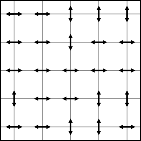
Figure 1. An illustration of Example 1.2 restricted to a small box.

[12] also shows the quenched invariance principle for ergodic elliptic environments under the moment condition

$$E[\big{(}\prod_{i=1}^{d}\omega(x,e_{i})\big{)}^{-p/d}]<\infty\quad\text{for some }\quad p>d.$$

Unlike the uniform elliptic case, one can find examples of ergodic elliptic balanced environment, where the invariance principle fails, as in the following two-dimensional example.

Example 1.3

For every point $z\in\mathbb{Z}^{2}$ we have Bernoulli variables $X^{z,ver}_{n},n=1,2,\ldots$ and $X^{z,hor}_{n},n=1,2,\ldots$. Those variables are all independent, and $P(X^{z,ver}_{n}=1)=P(X^{z,hor}_{n}=1)=3^{-n}$. Then, for every $z\in\mathbb{Z}^{2}$, if $X^{z,ver}_{n}=1$, then the $2^{n}$ vertices directly above $z$ all get chance $1-e^{-2n}$ to move in the vertical direction and chance $e^{-2n}$ to move in the horizontal direction. If $X^{z,hor}_{n}=1$, then the $2^{n}$ vertices directly to the right of $z$ all get chance $1-e^{-2n-1}$ to move in the horizontal direction and chance $e^{-2n-1}$ to move in the vertical direction. If a point hasn’t been spoken for, it gets probability $\frac{1}{4}$ to go in each direction. If a point has been spoken for more than once, it gets the highest value assigned to it.

It is not hard to prove that in Example 1.3, there exist $\alpha$ and $\beta$ positive such that for every large enough $T$, with probability at least $\alpha$, all movements in the time interval $[(1-\beta)T,T]$ are in vertical directions, and with probability at least $\alpha$, all movements in the time interval $[(1-\beta)T,T]$ are in horizontal directions. Furthermore, a.s. one can find infinitely many values of $T$ such that all movements in the time interval $[(1-\beta)T,T]$ are in vertical directions and infinitely many values of $T$ such that all movements in the time interval $[(1-\beta)T,T]$ are in horizontal directions. Obviously, such process cannot converge to a Brownian Motion, not even a degenerate one. It is also easy to show that the random walk in Example 1.3 is transient, even though it is two-dimensional.

The balanced assumption is essential for our proof and simplifies the argument greatly. In particular it implies that the walk is a martingale, which enables us to use the vast theory of martingales.

In particular, unlike the case of random conductances, we do not have to define and control a corrector. On the other hand, the existence and properties of an invariant measure for the process w.r.t. the point of view of the particle is a serious difficulty in our case, while it is simple in the case of random conductances.

We now define the process of the point of view of the particle, a notion which is standard in the literature of random walk in random environment, and is used in this paper. The environment viewed from the point of view of the particle is the Markov chain $\{\bar{\omega}_{n}\}_{n\in\mathbb{N}}$ given by

$$\bar{\omega}_{n}=\tau_{-X_{n}}\omega,$$

where $\tau$ is the shift on $\Omega$.

We can also view it as the Markov on $\Omega$ whose generator is

$$Lf(\omega)=\sum_{e:\|e\|=1}\omega(0,e)\big{[}f(\tau_{-e}\omega)-f(\omega)\big{]}.$$ (1.1)

The paper is organized as follows: in section 2 we introduce the rescaled process and give some estimate on the corresponding stopping times. Section 3 deals with the maximum principle for the rescaled process, while section 4 presents the stationary measure for the periodized environment. Then in Subsection 4.6 we repeat the arguments from [15] and [12] that lead to the existence of an invariant measure which is absolutely continuous w.r.t. $P$. In section 5 we prove Theorem 1.1. Finally, in Section 6 we we give a proof of the mean value inequality which is stated in Section 3 and used in Section 5.

2. The rescaled walk

In this section we define the rescaled walk, which is a useful notion in the study of non-elliptic balanced RWRE, and prove some basic facts about it.

Let $\{X_{n}\}_{n=0}^{\infty}$ be a nearest neighbor walk in $\mathbb{Z}^{d}$, i.e. a sequence in $\mathbb{Z}^{d}$ such that $\|X_{n+1}-X_{n}\|_{1}=1$ for every $n$. Let $\alpha_{n},n\geq 1$ be the coordinate that changes between $X_{n-1}$ and $X_{n}$, i.e. $\alpha(n)=i$ whenever $X_{n}-X_{n-1}=e_{i}$ or $X_{n}-X_{n-1}=-e_{i}$.

Definition 3

The stopping times $T_{k},k\geq 0$ are defined as follows: $T_{0}=0$. Then

$$T_{k+1}=\min\left\{t>T_{k}:\{\alpha(T_{k}+1),\ldots,\alpha(t)\}=\{1,\ldots,d\}\right\}\leq\infty.$$

We then define the rescaled random walk to be the sequence (no longer a nearest neighbor walk) $Y_{n}=X_{T_{n}}$. $\{Y_{n}\}$ is defined as long as $T_{n}$ is finite.

Lemma 2.1

$\mathbb{P}$-almost surely, $T_{k}<\infty$ for every $k$.

Lemma 2.2

There exists a constant $C$ such that for every $n$,

$$\mathbb{P}(T_{1}>n)<e^{-Cn^{\frac{1}{3}}}.$$

Note that due to lack of stationarity, Lemma 2.2 does not directly say anything about $T_{k+1}-T_{k}$ for large values of $k$. In Section 4 we will establish estimates for $T_{k+1}-T_{k}$ for large values of $k$.

proof of Lemma 2.2.

Note that $W_{n}=\sum_{i=1}^{d}X_{n}^{(i)}$ is a simple random walk, and whenever $W_{n}$ reaches a new value, $X_{n}$ visits a new point. Since the environment is i.i.d., whenever the walk is at a new point, its (annealed) probability of going in any direction, conditioned on its past, is bounded away from zero. Therefore,

$$\mathbb{P}\left(T_{1}>n\left|\max_{k\leq n}|W_{k}|\geq n^{\frac{1}{3}}\right.\right)\leq e^{-Cn^{\frac{1}{3}}},$$

and from standard SRW estimates,

$$\mathbb{P}\left(\max_{k\leq n}|W_{k}|<n^{\frac{1}{3}}\right)\leq e^{-Cn^{\frac{1}{3}}}.$$

Combined, we get the desired result. ∎

Proof of Lemma 2.1.

Assume that almost surely $T_{k}$ is finite, and we show that almost surely $T_{k+1}<\infty$. By the same argument as in the proof of Lemma 2.2, almost surely after time $T_{k}$ the walk $\{X_{n}\}$ will visit infinitely many new points. For every coordinate $i$, each time the walk visits a new point, conditioned on the past it has an annealed probability bounded away from zero to make a step in the direction $e_{i}$. Since infinitely many new points are visited, $\mathbb{P}(T_{k+1}<\infty|T_{k}<\infty)=1$. ∎

The annealed estimate in Lemma 2.2 can easily be turned into a quenched one.

Lemma 2.3

$$P\left(\omega:E_{\omega}(T_{1})>k\right)\leq e^{-Ck^{\frac{1}{3}}}.$$

Proof.

Note that if $E_{\omega}(T_{1})>k$, then

$$A(\omega)=\sum_{j=k/2}^{\infty}P_{\omega}(T_{1}>j)>k/2.$$

Now,

$$E(A(\omega))=\sum_{j=k/2}^{\infty}\mathbb{P}(T_{1}>j)\leq\sum_{j=k/2}^{\infty}e^{-Cj^{\frac{1}{3}}}\leq Ck^{3}e^{-Ck^{\frac{1}{3}}}$$

Markov’s inequality completes the proof.

∎

An immediate yet useful corollary of Lemma 2.3 is the following.

Lemma 2.4

For every $0<p<\infty$,

$$E\left[E_{\omega}(T_{1}^{p})\right]<\infty.$$

3. A maximum principle and a mean value inequality

In this section we prove a maximum principle which we will later use. It uses the same basic idea as the maximum principle of Kuo and Trudinger, [14], but the probabilistic and non-elliptic setting requires a new way of estimating the size of the set of the supporting hyperplanes, cf Lemma 3.4. We also state a mean value theorem, very similar to Theorem 12 of Guo and Zeitouni [12]. The proof of the mean value theorem is very similar to that of Theorem 12 of [12]. It appears in Section 6.

For $N\in\mathbb{N}$ and $k=k(N)\in(0,N)\cap\mathbb{Z}$, let $T_{1}^{(N)}=T_{1}^{(N,k)}=\min\big{(}T_{1},k\big{)}$. Let $h:\mathbb{Z}^{d}\to\mathbb{R}$ be a real valued function, and for every $z\in\mathbb{Z}^{d}$, let $L^{(N)}_{\omega}h(z):=h(z)-E_{\omega}^{z}[h(X_{T_{1}^{(N)}})]$.

Let $Q\subseteq\mathbb{Z}^{d}$ be finite and connected, and let $\partial^{(k)}Q=\{z\in\mathbb{Z}^{d}-Q:\exists_{x\in Q}\|z-x\|_{\infty}<k\}$.

We say that a point $z\in Q$ is exposed if there exists $\beta=\beta(z,h)\in\mathbb{R}^{d}$ such that $h(z)-\langle\beta,z\rangle\geq h(x)-\langle\beta,x\rangle$ for every $x\in Q\cup\partial^{(k)}Q$. We let $D_{h}$ be the set of exposed points. Further, we define the angle of vision $I_{h}(z)$ as follows:

$$I_{h}(z)=\left\{\beta\in\mathbb{R}^{d}:\forall_{x\in Q\cup\partial^{(k)}Q}h(x)\leq h(z)+\langle\beta,x-z\rangle\right\}.$$ (3.1)

This is the set of hyperplanes that touch the graph of $h$ at $(z,h(z))$ and are above the graph of $h$ all over $Q\cup\partial^{(k)}Q$. A point $z$ is exposed if and only if $I_{h}(z)$ is not empty.

Theorem 3.1 (Maximum Principle)

There exists $N_{0}$ such that for every $N>N_{0}$ and every $0<k<N$, every balanced environment $\omega$ and every $Q$ of diameter $N$, if for every $z\in Q$

$$P_{\omega}^{z}\big{(}T_{1}>k\big{)}<e^{-(\log N)^{3}}$$ (3.2)

then

$$\max_{z\in Q}h(z)-\max_{z\in\partial^{(k)}Q}h(z)\leq 6N\left(\sum_{z\in Q}{\bf 1}_{z\in D_{h}}|L^{(N)}_{\omega}h(z)|^{d}\right)^{\frac{1}{d}}$$

If $\Delta_{N}$ is a cube of side length $N$, then a more convenient way of writing the same thing is

$$\max_{z\in\Delta_{N}}h(z)-\max_{z\in\partial^{(k)}\Delta_{N}}h(z) \leq 6N^{2}\|{\bf 1}_{D_{h}}L^{(N)}_{\omega}h\|_{\Delta_{N},d}$$ (3.3)

$$\leq 6N^{2}\left\|\big{(}L^{(N)}_{\omega}h\big{)}^{+}\right\|_{\Delta_{N},d}$$

where, as in [12],

$$\|f\|_{\Delta_{N},p}=\left(\frac{1}{|\Delta_{N}|}\sum_{z\in\Delta_{N}}|f(z)|^{p}\right)^{\frac{1}{p}}$$

is the $L^{p}$ norm with respect to the uniform probability measure on $\Delta_{N}$.

Remark 1.

Note that if $\omega$ is sampled according to an i.i.d. environment satisfying Assumption 1, then by Lemma 2.3, (3.2) is almost surely satisfied for all large enough $N$, $k=(\log N)^{100}$ and any connected $Q$ of diameter $N$ that contains the origin. However, in this paper we also apply Theorem 3.1 to environments that are not i.i.d, namely to environments that are the periodized versions of i.i.d. environments.

We now state a mean value theorem, whose proof, which is essentially the same as the proof of Theorem 12 in [12], is postponed to Section 6. Let $B_{N}(x)=\{y\in\mathbb{Z}^{d}:|x-y|\leq N\}$, and $\bar{B}_{N}=B_{N}\cup\partial^{(\log N)^{100}}B_{N}$. For $u:\bar{B}_{N}\to\mathbb{R}$ let $L_{\omega}u(z)=u(z)-E_{\omega}^{z}(u(X_{1})).$

Theorem 3.2

For any $\sigma\in(0,1),0<p\leq d$ and $x_{0}\in\mathbb{Z}^{d}$ we can find $N_{0}=N_{0}(\sigma,p,d,x_{0})$ and $C=C(\sigma,p,d)$ such that $P$ almost surely if $N\geq N_{0}$ and $u$ on $\bar{B}_{N}(x_{0})$ satisfy

$$L_{\omega}u(x)=0,\quad x\in B_{N}(x_{0})$$

then

$$\max_{B_{\sigma N(x_{0})}}u\leq C\|u^{+}\|_{B_{N}(x_{0}),p}.$$

Proof of Theorem 3.1.

As in [14], we are mostly concerned with the angle of vision in any vertex, defined as follows: Let $z\in Q$. Recall The angle of vision $I_{h}(z)$ as defined as in (3.1).

Equivalently to [14], we will now state and use two simple geometrical lemmas. The proofs of these lemmas are postponed to immediately after the end of the current proof.

Lemma 3.3

For every $N$ and $0<k<N$,

$$\lambda\left(\bigcup_{z\in Q}I_{h}(z)\right)\geq\left|\frac{\max_{z\in Q}h(z)-\max_{z\in\partial^{(k)}Q}h(z)}{2N}\right|^{d},$$

where $\lambda$ is Lebesgue’s measure in $d$ dimensions.

Lemma 3.4

Almost surely, for every large enough $N$, every $Q$ of diameter $N$, every $\omega$ satisfying (3.2) and every $z\in Q\cap D_{h}$,

$$\lambda(I_{h}(z))\leq\left[\big{(}3L^{(N)}_{\omega}h(z)\big{)}^{+}\right]^{d}.$$ (3.4)

The theorem now follows once we note that

$$\lambda\left(\bigcup_{z\in\Delta_{N}}I_{h}(z)\right)\leq\sum_{z\in\Delta_{N}}\lambda(I_{h}(z)).$$

∎

Proof of Lemma 3.3.

This is identical to the proof of Lemma 2.2 in [14]. ∎

Proof of Lemma 3.4.

Let $\beta\in I_{h}(z)$. Fix $i\in\{1,\ldots,d\}.$ For a walk $\{X_{n}\}$ and $i=1,\ldots,d$, let $u_{i}=\min\{n:\alpha(n)=i\}\leq\infty$. We define the events

$$A_{i}^{(+)}=\{X_{u_{i}}-X_{u_{i}-1}=e_{i}\ \mbox{and}\ u_{i}\leq T_{1}^{(N)}\}$$

and

$$A_{i}^{(-)}=\{X_{u_{i}}-X_{u_{i}-1}=-e_{i}\ \mbox{and}\ u_{i}\leq T_{1}^{(N)}\}.$$

Let $W$ be a random variable which takes $+1$ with probability $1/2$ and $-1$ with the same probability, and is independent of the walk. Let $A_{i}^{0}$ be the event $A_{i}^{0}=\{u_{i}>k\}.$ We define

$$A_{i,N}^{(+)}=\big{(}A_{i}^{(+)}\cap(A_{i}^{0})^{c}\big{)}\cup\big{(}\{W=+1\}\cap(A_{i}^{0})\big{)}$$

and equivalently

$$A_{i,N}^{(-)}=\big{(}A_{i}^{(-)}\cap(A_{i}^{0})^{c}\big{)}\cup\big{(}\{W=-1\}\cap(A_{i}^{0})\big{)}.$$

Note that $P_{\omega}^{z}\big{(}A_{i,N}^{(+)}\big{)}=P_{\omega}^{z}\big{(}A_{i,N}^{(-)}\big{)}=1/2$ and that $A_{i,N}^{(+)}$ and $A_{i,N}^{(-)}$ are disjoint events. Therefore,

$$E_{\omega}^{z}(X_{T_{1}^{(N)}}|A_{i,N}^{(+)})-z=z-E_{\omega}^{z}(X_{T_{1}^{(N)}}|A_{i,N}^{(-)}).$$ (3.5)

Let $O^{(i)}_{\omega}(z)=E_{\omega}^{z}(X_{T_{1}^{(N)}}|A_{i,N}^{(+)})-z$.

$\beta\in I_{h}(z)$, and therefore $\langle\beta,x\rangle\geq h(z+x)-h(z)$ for every $x\in Q\cup\partial^{(k)}Q$. In particular, using the definition of $O^{(i)}_{\omega}(z)$ and (3.5),

$$\langle\beta,O^{(i)}_{\omega}(z)\rangle=\sum_{x\in Q\cup\partial^{(k)}Q}\langle\beta,x\rangle P_{\omega}^{z}(X_{T^{(N)}_{1}}=x+z|A_{i}^{(+)})$$ (3.6)

$$\geq \sum_{x\in Q\cup\partial^{(k)}Q}(h(x+z)-h(z))P_{\omega}^{z}(X_{T^{(N)}_{1}}=x|A_{i}^{(+)})$$

Equivalently,

$$\langle\beta,-O^{(i)}_{\omega}(z)\rangle=\sum_{x}\langle\beta,x\rangle P_{\omega}^{z}(X_{T^{(N)}_{1}}=x+z|A_{i}^{(-)})$$ (3.7)

$$\geq \sum_{x\in Q\cup\partial^{(k)}Q}(h(x+z)-h(z))P_{\omega}^{z}(X_{T^{(N)}_{1}}=x|A_{i}^{(-)})$$

in other words,

$$\sum_{x\in Q\cup\partial^{(k)}Q}(h(x+z)-h(z))P_{\omega}^{z}(X_{T^{(N)}_{1}}=x|A_{i}^{(-)})$$ (3.8)

$$\leq \langle\beta,O^{(i)}_{\omega}(z)\rangle$$

$$\leq -\sum_{x\in Q\cup\partial^{(k)}Q}(h(x+z)-h(z))P_{\omega}^{z}(X_{T^{(N)}_{1}}=x|A_{i}^{(+)}),$$

so whenever $\beta$ exists, $\langle\beta,O^{(i)}_{\omega}(z)\rangle$ is in an interval of length bounded by

$$- \left[\sum_{x}(h(x+z)-h(z))P_{\omega}^{z}(X_{T^{(N)}_{1}}=x|A_{i}^{(+)})+\sum_{x}(h(x+z)-h(z))P_{\omega}^{z}(X_{T_{1}}=x|A_{i}^{(-)})\right]$$

$$= 2\sum_{x}(h(z)-h(x+z))P_{\omega}^{z}(X_{T_{1}}=x)=2L^{(N)}_{\omega}h(z),$$

where the summation is over $x\in Q\cup\partial^{(k)}Q$. In particular, $L^{(N)}_{\omega}h(z)$ is non-negative if $\beta$ exists.

Therefore, $\lambda(I_{h}(z))$ is bounded by the volume of the parallelogram

$$L=\left\{\gamma\in\mathbb{R}^{d}:\forall_{i}\ 0\leq\big{\langle}\gamma,O^{(i)}_{\omega}(z)\big{\rangle}\leq 2L^{(N)}_{\omega}h(z)\right\}.$$

We thus need to estimate the volume of the parallelogram $L$. By standard linear algebra,

$$\lambda(L)=(2L^{(N)}_{\omega}h(z))^{d}\det(M^{-1})$$

where $M$ is the matrix whose columns are the vectors $O^{(i)}_{\omega}(z),\ 0\leq i\leq d$. Therefore, we need to estimate the value of the vectors $O^{(i)}_{\omega}(z)$.

Claim 3.5

for every $i$,

$$\|e_{i}-O^{(i)}_{\omega}(z)\|<e^{-(\log N)^{2}}.$$

Noting that the determinant is a continuous function, we get that (3.4) holds for all large enough $N$.

∎

Proof of Claim 3.5.

We calculate separately $O_{i}=\langle O^{(i)}_{\omega}(z),e_{i}\rangle$ and $O_{\not i}=O^{(i)}_{\omega}(z)-O_{i}$.

By the optional sampling theorem,

$$O_{i} = P_{\omega}^{z}(A_{i}^{(+)}|A_{i,N}^{(+)})\left[E_{\omega}^{z}(X_{T_{1}^{(N)}}|A_{i}^{(+)})-z\right]$$

$$+ P_{\omega}^{z}(A_{i}^{0}|A_{i,N}^{(+)})\left[E_{\omega}^{z}(X_{T_{1}^{(N)}}|A_{i,N}^{0})-z\right]$$

$$= P_{\omega}^{z}(A_{i}^{(+)}|A_{i,N}^{(+)}),$$

and therefore

$$|O_{i}-1|<e^{-(\log N)^{3}}$$ (3.9)

Using the optional sampling theorem one more time,

$$O_{\not i}=0.$$ (3.10)

The claim follows from (3.9) and (3.10).

∎

Remark 2.

Note that the rescaled walk is balanced in the following sense: For every $x$, $\omega$, $N$ and $k$,

$$\sum_{y}(y-x)P_{\omega}^{x}\left(X_{T_{1}^{(N)}}=y\right)=0.$$

4. Stationary measure for the periodized environment

As in [12] and [15], in this section we analyze the stationary measure of the walk on a periodized environment. Unlike those papers, here we consider a slight variation of the periodized environment, namely the reflected periodized environment, see Figure 2. The advantage of the choice of the reflected periodized environment over the one appearing in [12] and [15] is that every walk in the reflected periodized environment is (up to, possibly, some holding times) a legal walk in the original environment, which is not the case for the periodized environment appearing in [12] and [15]. This property of the reflected periodized environment will turn out to be very useful in Section 5.

Figure 2. The configuration under the letter A is the original configuration. The configuration under the letter B is the (reflected) periodized configuration with period 4, and the configuration under the letter C is the effective environment for the reflected random walk in the $4\times 4$ box. In places where there is only an arrow pointing in one direction, the walker stays put with probability $\frac{1}{2}.$ The origin in this picture is at the upper left corner.

The conclusion of this section is that for some $p>1$, the $L^{p}$ norm of the Radon-Nikodym derivative of a stationary measure with respect to the uniform measure on the period-cube is bounded as a function of the size of the period. As in [12] and [15] this will turn out to be the crucial step in the way of proving a CLT.

Differently from [12] and [15], we do it here with the stationary measure w.r.t. the rescaled walk and not w.r.t. the original walk, because the original walk does not necessarily obey the maximum principle (Theorem 3.1). The main idea is an idea that we learned from Theorem 5 of [12], but as we work with the rescaled walk, which is less regular than the original walk, the whole argument becomes significantly more complex. In Subsection 4.5 we transfer the result from stationary measures w.r.t. the rescaled walk to stationary measures w.r.t. the original walk.

4.1. Definition of the periodized environment

For every environment $\omega\in\Omega$ and $N\in\mathbb{N}$, we define the periodized environment $\omega^{(N)}$ as follows:

First we define $\omega^{(N)}(z)$ for $z$ in the cube $[0,2N-1]^{d}$: for $z=(z_{1},z_{2},\ldots,z_{d})$ we define $\omega^{(N)}(z)=\omega(z^{\prime})$ where

$$z^{\prime}=\big{(}\min(z_{1},2N-1-z_{1}),\min(z_{2},2N-1-z_{2}),\ldots,\min(z_{d},2N-1-z_{d})\big{)}.$$

Then for general $z$ we define $\omega^{(N)}(z)=\omega^{(N)}(z\mod 2N)$ where for every coordinate $i$ we define $(z\mod 2N)_{i}:=z_{i}-2N\cdot\lfloor\frac{z_{i}}{2N}\rfloor$. For a given environment $\omega$ and $N\in\mathbb{N}$, let $P_{\omega,N}$ be the uniform distribution over all $(2N)^{d}$ shifts of $\omega^{(N)}$. By $E_{\omega,N}$ we denote the expectation with respect to the distribution $P_{\omega,N}$. As in [12], due to the ergodic theorem and to the fact that the planes of reflection are a negligible set, $P$-almost surely $P_{\omega,N}$ converges weakly to $P$.

Note that the random walk in $\mathbb{Z}^{d}$ under $\omega^{(N)}$ corresponds to the reflected random walk on $\Delta_{N}=[0,N)^{d}$ under $\omega$, with some holding times. Indeed, if we define the function $f:\mathbb{Z}^{d}\to\Delta_{N}$ to be

$$f(z) = (g(z_{1}),\ldots,g(z_{d})),\mbox{ where}$$

$$g(x): = \min\big{(}x\mod 2N,2N-1-(x\mod 2N)\big{)},$$ (4.1)

then $\{f(X_{n})\}_{n=1}^{\infty}$ follows the law of a random walk on $\Delta_{N}$ under $\omega$ which is reflected at the boundaries of the cube, with a holding time when the random walker wants to leave the cube (again, see Figure 2).

Therefore, we can state and prove lemmas similar to Lemmas 2.2 and 2.3.

Lemma 4.1

There exists a constant $C$ such that for every $z$, every $N$ and every $k<2N$,

$$\int_{\Omega}P^{z}_{\omega^{(N)}}(T_{1}>k)dP(\omega)<e^{-Ck^{\frac{1}{3}}}.$$

Lemma 4.2

There exists a constant $C$ such that for every $z$, every $N$ and every $k<2N$,

$$P\left(\omega:E^{z}_{\omega^{(N)}}\left[(T_{1}\wedge\frac{N}{2})^{2}\right]>k\right)\leq e^{-Ck^{\frac{1}{6}}}.$$

Proof of Lemma 4.1.

The proof of Lemma 4.1 is basically the same as that of Lemma 2.2, except that we need to handle the fact that the environment is not i.i.d. and not even locally i.i.d. (consider, for example, any neighborhood of the point 0). As in the proof of Lemma 2.2, let $W_{n}=\sum_{i=1}^{d}X_{n}^{(i)}$. It is enough to show that, for two appropriate constants $C_{1}$ and $C_{2}$, the probability that the reflected walk $f(X_{k})$ (see display (4.1) for the definition) visits less than $C_{1}k^{1/3}$ points up to time $k$ is bounded by $e^{-C_{2}k^{1/3}}$.

To this end we consider separately the coordinates for which the point $z$ is closer than $\frac{k^{1/3}}{d}$ to the boundary of $\Delta_{N}$ and those for which the point $z$ is further than $\frac{k^{1/3}}{d}$ from the boundary. Without loss of generality, assume that $0\leq z^{(i)}<\frac{k^{1/3}}{d}$ for $1\leq i\leq\ell$, and that $\frac{k^{1/3}}{d}\leq z^{(i)}\leq N-\frac{k^{1/3}}{d}$ for $\ell<i\leq d$.

let $Z_{n}=W_{n}-W_{0}$ be the change in $(W_{\cdot})$. With probability greater than $1-\exp(-C_{2}k^{1/3})$, we get that

$$\max_{n\leq k}|Z_{n}|>3k^{1/3}.$$

Therefore, there exists a coordinate $i$ such that

$$\max_{n\leq k}|X_{n}^{(i)}-z^{(i)}|>\frac{3k^{1/3}}{d}.$$

Now, if $\ell<i\leq d$, then the first $\frac{k^{1/3}}{d}$ times that $|X_{n}^{(i)}-z^{(i)}|$ reaches a new maximum, $f(X_{n})$ visits a new point. If $1\leq i\leq\ell$, then whenever $|X_{n}^{(i)}-z^{(i)}|$ reaches $\frac{2k^{1/3}}{d}+1,\frac{2k^{1/3}}{d}+2,\ldots,\frac{3k^{1/3}}{d}$, the process $f(X_{n})$ visits a new point.

∎

Lemma 4.2 follows from Lemma 4.1 using the exact same calculation that yields Lemma 2.3 from Lemma 2.2. The different power ($1/6$ instead of $1/3$) stems from the power $2$ inside the expectation.

4.2. Empirical distribution of $E_{\omega}^{z}(T_{1}\wedge\frac{N}{2})$

For a number $N$ and an environment $\omega$, we denote $T=T(\omega,N):=\sqrt{E^{0}_{\omega}\big{(}\min(T_{1},\frac{N}{2})^{2}\big{)}}$ and for $z\in\mathbb{Z}^{d}$ we denote $T^{z}=T^{z}(\omega,N):=\sqrt{E^{z}_{\omega}\big{(}\min(T_{1},\frac{N}{2})^{2}\big{)}}$.

Lemma 4.3

Fix $1\leq p<\infty$. $P$-almost surely, for all $N$ large enough, for all $k\leq(\log\log N)^{100}$,

$$E_{\omega,N}(T^{p}\ ;\ T>k)\leq e^{-Ck^{1/3}}$$ (4.2)

where $E(X\ ;\ A)$ is defined to be $E(X\cdot{\bf 1}_{A})$.

Proof.

First, we show that there exists $c$ such that $P$-almost surely for all $N$ large enough,

$$E_{\omega,N}(T^{2p})<c.$$ (4.3)

Indeed, the LHS of (4.3) equals

$$\frac{1}{|\Delta_{2N}|}\sum_{z\in\Delta_{2N}}\left[T^{z}(\omega^{(N)},N)\right]^{2p}=\frac{1}{|\Delta_{2N}|}\sum_{z\in\Delta_{2N}}\left[E_{\omega^{(N)}}^{z}\big{(}\min(T_{1},\frac{N}{2})^{2}\big{)}\right]^{p}$$ (4.4)

Let $D_{N}=\{z\in\Delta_{2N}:\operatorname{dist}(z,\partial\Delta_{2N}>N^{0.7})\}$. Then for all $z\in D_{N}$, the probability that the random walk starting at $z$ reaches the boundary of $\Delta_{2N}$ before time $\frac{N}{2}$ decays like $e^{-cN^{0.4}}$. Therefore, for every $z\in D_{N}$, we get that

$$E_{\omega^{(N)}}^{z}\left[\min(T_{1},N/2)^{2}\right]\leq E_{\omega}^{z}\left[\min(T_{1},N/2)^{2}\right]+N^{2}e^{-N^{0.4}}\leq E_{\omega}^{z}T_{1}^{2}+N^{2}e^{-N^{0.4}}$$

and by applying Lemma 2.4 and the ergodic Theorem to the i.i.d. environment $\omega$ we get that a.s.

$$\sup\left\{\frac{1}{|\Delta_{2N}|}\sum_{z\in D_{N}}\left[E_{\omega^{(N)}}^{z}\big{(}\min(T_{1},\frac{N}{2})^{2}\big{)}\right]^{p}\ :\ N\in\mathbb{N}\right\}<\infty.$$ (4.5)

We thus need to bound

$$\frac{1}{|\Delta_{2N}|}\sum_{z\in\Delta_{2N}\setminus D_{N}}\left[E_{\omega^{(N)}}^{z}\big{(}\min(T_{1},\frac{N}{2})^{2}\big{)}\right]^{p}.$$

To this end, we use the fact that $|\Delta_{2N}\setminus D_{N}|/|\Delta_{2N}|<CN^{-0.3},$ Lemma 4.2 with choice of parameter $k=(\log N)^{20}$ and Borel-Cantelli.

Now that (4.3) has been established, by Cauchy-Schwarz, all we need to show is that $P$-almost surely, for all $N$ large enough, for all $k\leq(\log\log N)^{100}$,

$$P_{\omega,N}(T>k)\leq e^{-Ck^{1/3}}.$$ (4.6)

Note that

$$P_{\omega,N}(T>k)=\frac{1}{|\Delta_{2N}|}\sum_{z\in\Delta_{2N}}{\bf 1}_{\{T^{z}({\omega^{(N)}})>k\}}.$$

To prove (4.6), we need a second moment estimate. Let $\ell$ be an integer number, whose value will be determined later. Then

$$T^{z}(\omega)=\sum_{h=1}^{N/2}hP_{\omega}^{z}(T_{1}=h)=\sum_{h=1}^{\ell-1}hP_{\omega}^{z}(T_{1}=h)+\sum_{h=\ell}^{N/2}hP_{\omega}^{z}(T_{1}=h)$$ (4.7)

Write

$$B^{\ell,N/2}_{\omega}(z)=\sum_{h=\ell}^{N/2}hP_{\omega}^{z}(T_{1}=h)$$

and

$$B^{1,\ell}_{\omega}(z)=\sum_{h=1}^{\ell-1}hP_{\omega}^{z}(T_{1}=h).$$

By Lemma 4.1,

$$E\big{(}B^{\ell,N/2}_{\omega}(z)\big{)} = E\left(\sum_{h=\ell}^{N/2}hP_{\omega}^{z}(T_{1}=h)\right)$$ (4.8)

$$= \sum_{h=\ell}^{N/2}h\mathbb{P}^{z}(T_{1}=h)\leq C\ell^{3}e^{-\ell^{1/3}}.$$

Now set $\ell=\big{[}(\log N)^{60}\big{]}$. Using Markov’s inequality and a union bound, from (4.8) we see that

$$P\left(\exists_{z\in\Delta_{2N}}B^{\ell,{N/2}}_{\omega}(z)>1\right)C\leq|\Delta_{2N}|\ell^{3}e^{-\ell^{1/3}}\leq Ce^{-(\log N)^{18}}$$

and by Borel-Cantelli, with probability 1, $B^{\ell,N/2}_{\omega}(z)\leq 1$ for all $N$ large enough and every $z\in\Delta_{2N}$.

Therefore, it is sufficient to show that almost surely for all large enough $N$ and all $k\leq(\log\log N)^{100}$,

$$T_{N,k}:=\frac{1}{|\Delta_{2N}|}\left[\sum_{z\in\Delta_{2N}}{\bf 1}_{\{B^{1,\ell}_{\omega^{(N)}}(z)>k-1\}}\right]\leq e^{-Ck^{1/3}}.$$ (4.9)

From Lemma 4.2, for every $z\in\Delta_{2N}$,

$$P(B_{\omega^{(N)}}^{1,\ell}(z)>k-1)\leq P(T^{z}(\omega^{(N)})>k-1)\leq e^{-Ck^{1/3}}:=f(k).$$ (4.10)

Clearly, for every $z$ and $w$,

$$P\left(B_{\omega^{(N)}}^{1,\ell}(z)>k-1\ ;\ P(B_{\omega^{(N)}}^{1,\ell}(w)>k-1\right)$$ (4.11)

$$\leq P\big{(}B_{\omega^{(N)}}^{1,\ell}(z)>k-1\big{)}\leq f(k).$$

If, in addition, $||z-w||>\ell$, then by the i.i.d. nature of $P$ we get that

$$P\left(B_{\omega^{(N)}}^{1,\ell}(z)>k-1\ ;\ B_{\omega^{(N)}}^{1,\ell}(w)>k-1\right)$$ (4.12)

$$= P\big{(}B_{\omega^{(N)}}^{1,\ell}(z)>k-1\big{)}\cdot P\big{(}B_{\omega^{(N)}}^{1,\ell}(w)>k-1\big{)}.$$

Therefore, for $N$ large enough,

$${\texttt{var}}(T_{N,k})\leq\frac{1}{(2N)^{2d}}\left[\ell^{d}f(k)(2N)^{d}\right]\leq N^{-3d/4}f(k).$$

Thus by Chebichev’s inequality,

$$P(T_{N,k}>2f(k))\leq N^{-3d/4}/f(k),$$

and a union bound says that

$$P\left(\exists_{k\leq(\log\log N)^{100}}\ :\ T_{N,k}>2f(k)\right)$$

$$\leq N^{-3d/4}\cdot(\log\log N)^{100}\cdot e^{C(\log\log N)^{100/3}}$$

$$\leq N^{-3d/5}.$$

Remembering that $d\geq 2$, Borel-Cantelli now finishes the proof.

∎

4.3. Stationary measure

Let $P_{N}$ be the uniform distribution on $\Delta_{N}$. Let $H_{N}=H_{N}(\omega)$ be a stationary measure for the Markov process $\{f(Y_{n})\}_{n=1}^{\infty}$ on $\Delta_{N}$ where $\{Y_{n}\}_{n=1}^{\infty}$ is the rescaled walk on $\mathbb{Z}^{d}$ under the environment $\omega^{(N)}$ and $f$ is as in (4.1) (note that due to the non irreducibility of the Markov chain, there may be more than one stationary measure. In this case, $H_{N}$ is arbitrarily chosen among the stationary measures. Also note that by Lemma 4.2, $P$-almost surely for all large enough $N$, the process $\{Y_{n}\}_{n=0}^{\infty}$ is well defined), and let $\Phi_{N}=\Phi_{N}(\omega)=\frac{dH_{N}}{dP_{N}}$ be the Radon-Nikodym derivative of $H_{N}$. The main purpose of this section is the following lemma, whose proof will be completed in the next subsection.

Lemma 4.4

Fix $p=\frac{d}{d-1}$. There exists a constant $C_{\ref{eq:lpbound}}$ such that for almost every $\omega$, we have that

$$\limsup\left\{\|\Phi_{N}\|_{\Delta_{N},p}\ :\ N=1,2,\ldots\right\}\leq C_{\ref{eq:lpbound}}.$$ (4.13)

We begin with three definitions and a basic lemma, which will serve as the input for the main step.

Definition 4

The average step size at scale $N$, denoted by $O_{N}=O_{N}(\omega)$ is defined to be

$$O_{N}:=\sqrt{E_{H_{N}}\big{[}(T_{1}\wedge N/2)^{2}\big{]}}=\left(\frac{1}{|\Delta_{N}|}\sum_{z\in\Delta_{N}}\Phi_{N}(z)E_{\omega^{(N)}}^{z}\big{[}(T_{1}\wedge N/2)^{2}\big{]}\right)^{1/2}.$$ (4.14)

At this point we remind the reader that $\{X_{n}\}$ denotes the original walk, while $\{Y_{n}\}$ denotes the rescaled walk. As in [12] we define the following stopping times.

Definition 5

We define $S_{1}=S_{1}(N):=\inf\{n:\|Y_{n}-Y_{0}\|_{\infty}\geq 2N\}$ and recursively $S_{k+1}=S_{k+1}(N):=\inf\{n>S_{k}:\|Y_{n}-Y_{S_{k}}\|_{\infty}\geq 2N\}$. If $S_{k}$ is not well defined (either because the rescaled walk is not well defined or because the walk never leaves the neighborhood of $S_{k-1}$), we set $S_{k}$ to infinity, as well as $S_{j},j>k$.

We also define corresponding stopping times for the original walk $\{X_{n}\}$.

Definition 6

We define $\Gamma_{k}=\Gamma_{k}(N)=T_{S_{k}}$, i.e. the time when $S_{k}$ occurs in the clock of the original walk.

From the fact that $\{X_{n}\}$ is a martingale whose step size is one, we get the following simple estimate.

Lemma 4.5

There exists a constant $C$ such that for every $N$ and almost every $\omega$,

$$\sum_{k=1}^{\infty}P_{\omega^{(N)}}(\Gamma_{k}<CkN^{2})<\infty.$$ (4.15)

Furthermore,

$$\operatorname{esssup}\left\{\sum_{k=1}^{\infty}P_{\omega^{(N)}}(\Gamma_{k}<CkN^{2})\right\}<\infty,$$ (4.16)

where the essential supremum is taken w.r.t. the measure $P$ on $\omega$.

Proof.

Note that $\Gamma_{k}$ is a stopping time for every $k$, and that $\|X_{\Gamma_{k+1}}-X_{\Gamma_{k}}\|\geq 2N$. Now remember that $\{X_{n}\}$ is a martingale, and that the variance of its increments is 1. By Doob’s inequality, there exists $C_{\ref{eq:doob}}$ such that for every balanced $\omega$ and all $k$,

$$P_{\omega}\left(\left.\Gamma_{k+1}-\Gamma_{k}>C_{\ref{eq:doob}}N^{2}\ \right|X_{1},\ldots,X_{\Gamma_{k}}\right)>1/2.$$ (4.17)

If we now take $C=C_{\ref{eq:doob}}/4$, then by (4.17) and Cramèr’s Theorem we get that for every balanced $\omega$,

$$P_{\omega}(\Gamma_{k}<CkN^{2})$$ (4.18)

$$\leq P_{\omega}\left(\mbox{There exist more than $\frac{3k}{4}$ values of $n$ up to $k$ s.t. }\Gamma_{n+1}-\Gamma_{n}\leq C_{\ref{eq:doob}}N^{2}\right)$$

$$\leq e^{-C_{\ref{eq:cramer}}k}.$$

(4.16) follows.

∎

4.4. A bootstrap argument

In this subsection we perform a bootstrap argument that will simultaneously control $O_{N}$ and prove Lemma 4.4. The argument is composed of two lemmas. The first, Lemma 4.7, an adaptation of Theorem 5 of [12], bounds $\|\Phi_{N}\|_{\Delta_{N},p}$ in terms of $O_{N}$ and the second, Lemma 4.8, bounds $O_{N}$ in terms of $\|\Phi_{N}\|_{\Delta_{N},p}$.

We start with an a priori bound.

Claim 4.6

$P$-almost surely, $O_{N}\leq(\log N)^{4}$ for all $N$ large enough.

Proof.

This follows from the fact that $|\Delta_{N}|=N^{d}$ and from Lemma 4.1, the same way Lemma 2.3 is proven. ∎

Lemma 4.7

$P$-almost surely, there exists a constant $C_{1}$ such that for every $N$ large enough,

$$\|\Phi_{N}\|_{\Delta_{N},p}<C_{1}\cdot O_{N},$$

where, as before, $p=\frac{d}{d-1}$.

Lemma 4.8

$P$-almost surely, there exists a constant $C_{2}$ such that for every $N$ large enough and every $k<(\log N)^{5}$, if

$$\|\Phi_{N}\|_{\Delta_{N},p}<k$$

then

$$O_{N}<C_{2}(\log k)^{4}.$$

Proof of Lemma 4.4.

The combination of Claim 4.6 and Lemmas 4.7 and 4.8 yields that for all $N$ large enough, $O_{N}\leq C_{1}C_{2}(\log O_{N})^{4}$, and therefore $\sup\{O_{N}:N=1,2,\ldots\}<\infty$. Another application of Lemma 4.7 yields (4.13). ∎

Proof of Lemma 4.8.

Let $j=(\log k)^{4}$, and let $f(z)=E_{\omega^{(N)}}^{z}\big{[}(T_{1}\wedge N/2)^{2}\big{]}$. Then

$$O_{N}^{2}=\frac{1}{N^{d}}\sum_{z\in\Delta_{N}}\Phi_{N}(z)f(z) =$$

$$\frac{1}{N^{d}}\sum_{z\in\Delta_{N}}\Phi_{N}(z)f(z){\bf 1}_{f(z)\leq j} + \frac{1}{N^{d}}\sum_{z\in\Delta_{N}}\Phi_{N}(z)f(z){\bf 1}_{f(z)>j}$$

$$\leq j + \|\Phi_{N}\|_{\Delta_{N},p}\|f(z){\bf 1}_{f(z)>j}\|_{\Delta_{N},d}$$

$$\leq j+ke^{-Cj^{1/3}} \leq 2j$$

where the one before last inequality follows from Hölder’s inequality, Lemma 4.3 and the assumption that $\|\Phi_{N}\|_{\Delta_{N},p}<k$, and the last inequality follows from the fact that $j^{1/3}>\log k$.

∎

Proof of Lemma 4.7.

The argument is based on the proof of Theorem 5 in [12]. Let $h:\Delta_{2N}\to\mathbb{R}^{+}$ be a test function. We extend $h$ to the entire $Z^{d}$ by $h(x):=h(x\mod 2N)$.

We remember that $\{Y_{\cdot}\}$ is the rescaled walk, and extend $\Phi_{N}$ to $\Delta_{2N}$ by $\Phi_{N}(x):=\Phi_{N}(f(x))$ for $f$ as in (4.1). The extended $\Phi_{N}$ is the Radon-Nikodym derivative of the measure $\tilde{H}$ defined as $\tilde{H}(x)=\frac{1}{2^{d}}H_{N}(f(x))$. Note that $\tilde{H}$ is stationary with respect to the (periodized) random walk on $\Delta_{2N}$. Then

$$\frac{1}{(2N)^{d}}\sum_{z\in\Delta_{2N}}\Phi_{N}(z)h(z)$$

$$= \frac{O_{N}}{N^{2}}\sum_{z\in\Delta_{2N}}\frac{\Phi_{N}(z)}{(2N)^{d}}\sum_{j=0}^{\infty}E_{\omega^{(N)}}^{z}\left(1-\frac{O_{N}}{N^{2}}\right)^{j}h(Y_{j})$$

$$= \frac{O_{N}}{N^{2}}\sum_{z\in\Delta_{2N}}\frac{\Phi_{N}(z)}{(2N)^{d}}\sum_{m=0}^{\infty}\sum_{j=S_{m}}^{S_{m+1}-1}E_{\omega^{(N)}}^{z}\left(1-\frac{O_{N}}{N^{2}}\right)^{j}h(Y_{j})$$

$$\leq \frac{O_{N}}{N^{2}}\sum_{z\in\Delta_{2N}}\frac{\Phi_{N}(z)}{(2N)^{d}}\sum_{m=0}^{\infty}E_{\omega^{(N)}}^{z}\left(1-\frac{O_{N}}{N^{2}}\right)^{S_{m}}E_{\omega^{(N)}}^{Y_{S_{m}}}\sum_{j=0}^{S_{m+1}-S_{m}-1}h(Y_{j})$$

$$\leq \frac{O_{N}}{N^{2}}\left(\max_{z\in\Delta_{2N}}E_{\omega^{(N)}}^{z}\sum_{j=0}^{S_{1}-1}h(Y_{j})\right)\left(\sum_{z\in\Delta_{2N}}\frac{\Phi_{N}(z)}{(2N)^{d}}\sum_{m=0}^{\infty}E_{\omega^{(N)}}^{z}\left(1-\frac{O_{N}}{N^{2}}\right)^{S_{m}}\right)$$

We use the following claim, whose proof will be given at the end of the proof of the lemma.

Claim 4.9

$$\max_{z\in\Delta_{2N}}E_{\omega^{(N)}}^{z}\sum_{j=0}^{S_{1}-1}h(Y_{j})\leq CN^{2}\|h\|_{\Delta_{2N},d}.$$ (4.20)

We now estimate the remaining term, namely

$$\sum_{z\in\Delta_{2N}}\frac{\Phi_{N}(z)}{(2N)^{d}}\sum_{m=0}^{\infty}E_{\omega^{(N)}}^{z}\left(1-\frac{O_{N}}{N^{2}}\right)^{S_{m}}.$$

Note that this is

$$\sum_{m=0}^{\infty}E_{\tilde{H}_{N}}\left(1-\frac{O_{N}}{N^{2}}\right)^{S_{m}}=\sum_{m=0}^{\infty}E_{H_{N}}\left(1-\frac{O_{N}}{N^{2}}\right)^{S_{m}},$$

and that $H_{N}$ is a stationary distribution for $\{f(Y_{\cdot})\}$. In particular, the sequence $\{T_{k}-T_{k-1}\}$ is stationary under $H_{N}$, and $E_{H_{N}}\big{[}(T_{k}-T_{k-1})^{2}\big{]}=O_{N}^{2}$ for every $k$.

Now, for a given $m>0$,

$$E_{H_{N}}\left(1-\frac{O_{N}}{N^{2}}\right)^{S_{m}}$$ (4.21)

$$\leq \left(1-\frac{O_{N}}{N^{2}}\right)^{\frac{N^{2}}{O_{N}}(\log m)^{4}}+P_{H_{N}}\left(S_{m}<\frac{N^{2}}{O_{N}}(\log m)^{4}\right)$$

$$\leq 2e^{-(\log m)^{4}}+P_{H_{N}}\left(S_{m}<\frac{N^{2}}{O_{N}}(\log m)^{4}\right).$$

Let $C_{\ref{lem:gamma_big}}$ be the constant from Lemma 4.5. Then

$$P_{H_{N}}\left(S_{m}<\frac{N^{2}}{O_{N}}(\log m)^{4}\right)$$

$$\leq P_{H_{N}}\left(\Gamma_{m}<C_{\ref{lem:gamma_big}}mN^{2}\right)+P_{H_{N}}\left(S_{m}<\frac{N^{2}}{O_{N}}(\log m)^{4}\ ;\ \Gamma_{m}\geq C_{\ref{lem:gamma_big}}mN^{2}\right)$$

Lemma 4.5 takes care of the first summand, so all we have left to do is to control the second summand. By Markov’s inequality,

$$P_{H_{N}}\left(S_{m}<\frac{N^{2}}{O_{N}}(\log m)^{4}\ ;\ \Gamma_{m}\geq C_{\ref{lem:gamma_big}}mN^{2}\right)$$ (4.23)

$$\leq P_{H_{N}}\left(T_{\left[\frac{N^{2}}{O_{N}}(\log m)^{4}\right]}\geq C_{\ref{lem:gamma_big}}mN^{2}\right)$$

$$\leq \frac{E_{H_{N}}\left[\left(T_{\left[\frac{N^{2}}{O_{N}}(\log m)^{4}\right]}\right)^{2}\right]}{C_{\ref{lem:gamma_big}}^{2}m^{2}N^{4}}$$

and

$$E_{H_{N}}\left[\left(T_{\left[\frac{N^{2}}{O_{N}}(\log m)^{4}\right]}\right)^{2}\right]=E_{H_{N}}\left[\left(\sum_{i=1}^{\left[\frac{N^{2}}{O_{N}}(\log m)^{4}\right]}T_{i}-T_{i-1}\right)^{2}\right]$$

$$= \sum_{i=1}^{\left[\frac{N^{2}}{O_{N}}(\log m)^{4}\right]}\sum_{j=1}^{\left[\frac{N^{2}}{O_{N}}(\log m)^{4}\right]}E_{H_{N}}[(T_{i}-T_{i-1})(T_{j}-T_{j-1})]$$

$$\leq \frac{N^{4}}{O_{N}^{2}}(\log m)^{8}\cdot O_{N}^{2}=N^{4}(\log m)^{8}$$

Substituting in (4.23), we get that

$$P_{H_{N}}\left(S_{m}<\frac{N^{2}}{O_{N}}(\log m)^{4}\ ;\ \Gamma_{m}\geq C_{\ref{lem:gamma_big}}mN^{2}\right)\leq\frac{(\log m)^{8}}{m^{2}C_{\ref{lem:gamma_big}}^{2}}$$

and combined with (4.21), (4.4) and Lemma 4.5, we get that for every test function $h$,

$$\frac{1}{(2N)^{d}}\sum_{z\in\Delta_{2N}}\Phi_{N}(z)h(z)\leq C_{1}\|h\|_{\Delta_{2N},d}O_{N}.$$

The duality of $L^{d}$ and $L^{p}$ now gives that $\|\Phi_{N}\|_{\Delta_{N},p}=\|\Phi_{N}\|_{\Delta_{2N},p}\leq C_{1}O_{N}.$ ∎

Proof of Claim 4.9.

We need to show (4.20). We first estimate

$$\max_{z\in\Delta_{2N}}E_{\omega^{(N)}}^{z}\sum_{j=0}^{S_{1}-1}h(Y^{(N)}_{j})$$

Where the walk $Y^{(N)}_{j}$ is defined by $Y^{(N)}_{j}=X_{T^{(N)}_{j}}$, with $T_{1}^{(N)}:=\min(T_{1},N/2)$ and

$$T_{k+1}^{(N)}:=\min\big{\{}\{t>T_{k}^{(N)}\ :\ \{\alpha(T_{k}^{(N)}+1),\ldots,\alpha(t)\}=\{1,\ldots,d\}\}\cup\{T_{k}^{(N)}+N/2\}\big{\}}.$$

We fix $z\in\Delta_{2N}$, and define the stopping time $T^{z}=\min\{j\ :\ Y^{(N)}_{j}\notin z+\Delta_{2N}\}$ and the function

$$f^{z}(x)=E_{\omega^{(N)}}^{x}\sum_{j=0}^{T^{z}-1}h(Y^{(N)}_{j}).$$

Then $L^{(N)}f^{z}=h$. Almost surely, for all $N$ large enough, Condition (3.2) with $k=N/2$ is satisfied by Lemma 4.2, and therefore by Theorem 3.1,

$$E_{\omega^{(N)}}^{z}\sum_{j=0}^{S_{1}-1}h(Y^{(N)}_{j})=f^{z}(z)\leq CN^{2}\|h\|_{\Delta_{2N},d}.$$

Therefore, all we need is to control

$$E_{\omega^{(N)}}^{z}\left[\left|\sum_{j=0}^{S_{1}-1}h(Y^{(N)}_{j})-\sum_{j=0}^{S_{1}-1}h(Y_{j})\right|\right].$$

Now,

$$E_{\omega^{(N)}}^{z}\left[\left|\sum_{j=0}^{S_{1}-1}h(Y^{(N)}_{j})-\sum_{j=0}^{S_{1}-1}h(Y_{j})\right|^{2}\right]\leq CN^{4}\max_{z\in\Delta_{2N}}h^{2}(z)$$

and

$$P_{\omega^{(N)}}^{z}\left[\left|\sum_{j=0}^{S_{1}-1}h(Y^{(N)}_{j})-\sum_{j=0}^{S_{1}-1}h(Y_{j})\right|\neq 0\right]\leq N^{2}e^{-cN^{1/3}}.$$

¿From Cauchy-Schwarz, we see that

$$E_{\omega^{(N)}}^{z}\left[\left|\sum_{j=0}^{S_{1}-1}h(Y^{(N)}_{j})-\sum_{j=0}^{S_{1}-1}h(Y_{j})\right|\right]\leq CN^{4}e^{-cN^{1/3}}\max_{z\in\Delta_{2N}}h(z).$$ (4.24)

Noting that the size of the space $\Delta_{2N}$ is $(2N)^{d}$, we get that

$$\max_{z\in\Delta_{2N}}h(z)=\|h\|_{\Delta_{2N},\infty}\leq(2N)^{d}\|h\|_{\Delta_{N},d}.$$

With (4.24) we are now done.

∎

4.5. A stationary measure for the original random walk on $\Delta_{N}$

Fix $p^{\prime}$ to be strictly between $1$ and $p$. In Lemma 4.4 we controlled the $L^{p}$ norm of a stationary measure w.r.t. the rescaled random walk. We now use Lemma 4.4 to control the $L^{p^{\prime}}$ norm of a stationary measure w.r.t. the original random walk.

Lemma 4.10

There exists $C$ such that $P$-almost surely for all $N$ large enough, every probability measure $Q_{N}$ which is stationary with respect to the original reflected random walk on $\Delta_{N}$ satisfies

$$\left\|\frac{dQ_{N}}{dP_{N}}\right\|_{\Delta_{N},p^{\prime}}<C.$$

Proof.

First note that due to the convexity of the norm $\|\cdot\|_{\Delta_{N},p^{\prime}}$, we may assume without loss of generality that the measure $Q_{N}$ is ergodic. Then the random walk is irreducible on $\operatorname{supp}Q_{N}$. It is also clear that if the random walk starts at a point in $\operatorname{supp}Q_{N}$, it will stay in $\operatorname{supp}Q_{N}$ forever. Therefore, there exists a measure $H_{N}$ which is supported on (a subset of) $\operatorname{supp}Q_{N}$ and is stationary with respect to the rescaled random walk.

Now consider the following random walk $\{X_{n}\}_{n=0}^{\infty}$ on $\Delta_{N}$: the initial point $X_{0}$ is determined according to the distribution $H_{N}$, and the walk continues according to the quenched kernel $\omega$ on $\Delta_{N}$, reflected at the boundary.

For $i=0,\ldots,$ we define the measure (not a probability measure) $F_{i}$ on $\Delta_{N}$ by

$$F_{i}(x)=\sum_{z\in\Delta_{N}}H_{N}(z)P_{\omega}^{z}(X_{i}=x\ ;\ T_{1}>i).$$

Claim 4.11

For $P$-almost every $\omega$ and all $N$ large enough, the sum

$$\sum_{i=0}^{\infty}F_{i}$$

converges to a finite measure $F$. Furthermore, $\|F\|_{1}=E_{H_{N}}(T_{1})$ and $F$ is stationary w.r.t. the (original) random walk.

Since the random walk is irreducible on $\operatorname{supp}Q_{N}$, there is a unique stationary measure for the original random walk, and therefore $Q_{N}=F/E_{H_{N}}(T_{1})$. As $E_{H_{N}}(T_{1})>1$, we get that

$$\left\|\frac{dQ_{N}}{dP_{N}}\right\|_{\Delta_{N},p^{\prime}}\leq\sum_{i=0}^{\infty}\left\|\frac{dF_{i}}{dP_{N}}\right\|_{\Delta_{N},p^{\prime}}.$$

Therefore, we want to estimate $\left\|\frac{dF_{i}}{dP_{N}}\right\|_{\Delta_{N},p^{\prime}}$ for given $i$.

We first estimate $\left\|\frac{dF_{i}}{dP_{N}}\right\|_{\Delta_{N},p}.$ Note that

$$F_{i}(x)\leq G_{i}(x):=\sum_{z\in\Delta_{N}}H_{N}(z)P_{\omega}^{z}(X_{i}=x),$$

$$G_{i}(x) = \sum_{z\in\Delta_{N}\ :\ |z-x|\leq i}H_{N}(z)P_{\omega}^{z}(X_{i}=x)$$

$$\leq \sum_{z\in\Delta_{N}\ :\ |z-x|\leq i}H_{N}(z).$$

Therefore

$$\left(G_{i}(x)\right)^{p}\leq(2i+1)^{d(p-1)}\sum_{z\in\Delta_{N}\ :\ |z-x|\leq i}(H_{N}(z))^{p},$$

so

$$\left\|\frac{dF_{i}}{dP_{N}}\right\|_{\Delta_{N},p}\leq\left\|\frac{dG_{i}}{dP_{N}}\right\|_{\Delta_{N},p}\leq(2i+1)^{d}\left\|\frac{dH_{N}}{dP_{N}}\right\|_{\Delta_{N},p}.$$ (4.25)

Let $p^{\prime\prime}$ be such that $\frac{1}{p^{\prime\prime}}+\frac{p^{\prime}}{p}=1$.

We also want to estimate $\left\|\frac{dF_{i}}{dP_{N}}\right\|_{\Delta_{N},1}.$

$$\left\|\frac{dF_{i}}{dP_{N}}\right\|_{\Delta_{N},1}=\sum_{x\in\Delta_{N}}F_{i}(x) = \sum_{x\in\Delta_{N}}\sum_{z\in\Delta_{N}}H_{N}(z)P_{\omega}^{z}(X_{i}=x\ ;\ T_{1}>i)$$

$$= \sum_{z\in\Delta_{N}}H_{N}(z)P_{\omega}^{z}(T_{1}>i)\leq e^{-Ci^{1/3}},$$

where the last inequality follows from Lemma 4.1.

Now let

$$Y(x)={\bf 1}_{\left\{\frac{F_{i}(x)}{P_{N}(x)}>1\right\}}$$

and let $X_{1}(x)=Y(x)\cdot\frac{F_{i}(x)}{P_{N}(x)}$ and $X_{2}(x)=(1-Y(x))\cdot\frac{F_{i}(x)}{P_{N}(x)}$. Since $\frac{dF_{i}}{dP_{N}}=X_{1}+X_{2}$, we need to estimate $\|X_{1}\|_{\Delta_{N},p^{\prime}}$ and $\|X_{2}\|_{\Delta_{N},p^{\prime}}$.

Note that $X_{2}(x)\leq 1$ for every $x$, and therefore, $X_{2}^{p^{\prime}}(x)\leq X_{2}(x)$. Therefore, $\|X_{2}\|_{\Delta_{N},p^{\prime}}\leq\|X_{2}\|_{\Delta_{N},1}^{1/p^{\prime}}\leq\exp\big{(}-(C/p^{\prime})i^{1/3}\big{)}.$

Note also that $Y(x)\in\{0,1\}$ and thus $Y^{p^{\prime\prime}}=Y$, so, using Markov’s inequality,

$$\|Y\|_{\Delta_{N},p^{\prime\prime}}^{p^{\prime\prime}}=\|Y\|_{\Delta_{N},1}\leq\left\|\frac{dF_{i}}{dP_{N}}\right\|_{\Delta_{N},1}\leq\exp\big{(}-Ci^{1/3}\big{)},$$

so $\|Y\|_{\Delta_{N},p^{\prime\prime}}\leq\exp\big{(}-(C/p^{\prime\prime})i^{1/3}\big{)}.$ Then by Hölder’s inequality,

$$\|X_{1}\|_{p^{\prime}}^{p^{\prime}}\leq\left\|\frac{dF_{i}}{dP_{N}}\right\|_{\Delta_{N},p}^{p^{\prime}}\cdot\|Y\|_{p^{\prime\prime}}\leq\|H_{N}\|_{p}^{p^{\prime}}\cdot(2i+1)^{dp^{\prime}}\exp\big{(}-(C/p^{\prime\prime})i^{1/3}\big{)}.$$

We get that for appropriate constants $C_{1}$ and $C_{2}$,

$$\left\|\frac{dF_{i}}{dP_{N}}\right\|_{p^{\prime}}\leq C_{1}(2i+1)^{d}\exp\big{(}-C_{2}i^{1/3}\big{)}\cdot\|H_{N}\|_{p}.$$

The lemma now follows from Lemma 4.4 and the fact that

$$\sum_{i=0}^{\infty}C_{1}(2i+1)^{d}\exp\big{(}-C_{2}i^{1/3}\big{)}<\infty.$$

∎

Proof of Claim 4.11.

First of all,

$$\|F_{i}\|_{1}=\sum_{x\in\Delta_{N}}F_{i}(x) = \sum_{x\in\Delta_{N}}\sum_{z\in\Delta_{N}}H_{N}(z)P_{\omega}^{z}(X_{i}=x\ ;\ T_{1}>i)$$

$$= \sum_{z\in\Delta_{N}}\sum_{x\in\Delta_{N}}H_{N}(z)P_{\omega}^{z}(X_{i}=x\ ;\ T_{1}>i)$$

$$= \sum_{z\in\Delta_{N}}H_{N}(z)P_{\omega}^{z}(T_{1}>i)=P_{H_{N}}(T_{1}>i).$$

Therefore $\sum_{i=1}^{\infty}F_{i}$ converges and $\|F\|_{1}=E_{H_{N}}(T_{1})$.

To show stationarity, we do the following calculation. Fix $x\in\Delta_{N}$.

$$\sum_{y\in\Delta_{N}}F(y)P_{\omega}^{y}(X_{1}=x) = \sum_{i=0}^{\infty}\sum_{y\in\Delta_{N}}F_{i}(y)P_{\omega}^{y}(X_{1}=x)$$

$$=\sum_{i=0}^{\infty}\sum_{z\in\Delta_{N}}H_{N}(z)P_{\omega}^{z}(X_{i+1}=x\ ;\ T_{1}>i) = \sum_{j=1}^{\infty}\sum_{z\in\Delta_{N}}H_{N}(z)P_{\omega}^{z}(X_{j}=x\ ;\ T_{1}\geq j)$$

$$=\sum_{j=1}^{\infty}\sum_{z\in\Delta_{N}}H_{N}(z)P_{\omega}^{z}(X_{j}=x\ ;\ T_{1}>j) + \sum_{j=1}^{\infty}\sum_{z\in\Delta_{N}}H_{N}(z)P_{\omega}^{z}(X_{j}=x\ ;\ T_{1}=j)$$

$$=\sum_{j=1}^{\infty}F_{j}(x)+\sum_{z\in\Delta_{N}}H_{N}(z)P_{\omega}^{z}(X_{T_{1}}=x) = \sum_{j=1}^{\infty}F_{j}(x)+H_{N}(x)=F(x),$$

where in the one before last step we used the stationarity of $H_{N}$ with respect to the rescaled random walk. ∎

We get a useful corollary.

Corollary 4.12

There exists $\Phi>0$ which depends only on $P$ such that $P$-almost surely for all large enough $N$, every stationary measure $Q_{N}$ with respect to the reflected random walk in $\Delta_{N}$ under the environment $\omega$ satisfies $|\operatorname{supp}Q_{N}|\geq\Phi|\Delta_{N}|$.

Proof.

By Lemma 4.10,

$$\left\|\frac{dQ_{N}}{dP_{N}}\right\|_{\Delta_{N},p^{\prime}}<C^{\prime}.$$

Now, by Hölder’s inequality, for $p^{\prime\prime}$ such that $1/p^{\prime}+1/p^{\prime\prime}=1$,

$$1=\left\|\frac{dQ_{N}}{dP_{N}}\right\|_{\Delta_{N},1}\leq\left\|\frac{dQ_{N}}{dP_{N}}\right\|_{\Delta_{N},p^{\prime}}\cdot\left\|{\bf 1}_{\operatorname{supp}Q_{N}}\right\|_{\Delta_{N},p^{\prime\prime}}\leq C^{\prime}\left(\frac{|\operatorname{supp}Q_{N}|}{|\Delta_{N}|}\right)^{1/p^{\prime\prime}}.$$

Therefore,

$$\frac{|\operatorname{supp}Q_{N}|}{|\Delta_{N}|}\leq\frac{1}{{C^{\prime}}^{p^{\prime\prime}}}=:\Phi.$$

∎

4.6. Existence of an invariant measure.

Identically to [12] and [15], from Lemma 4.10 we can prove that there exists a measure $Q$ on $\Omega$ such that $Q\ll P$ and $Q$ is stationary with respect to the random walk viewed from the point of view of the particle. In order to keep this paper self-contained, we state and prove it as Proposition 4.14 below.

Once we established $Q$, using Feller-Lindeberg’s central limit theorem, see e.g. [11], we get the following fact.

Fact 4.13

If in addition $Q$ is ergodic, then $Q$ almost surely the quenched law $P_{\omega}^{0}$ satisfies an invariance principle with a non-random diagonal, non-degenerate diffusion matrix.

Proof that the matrix is diagonal and non-degenerate.

The proof that the matrix is diagonal is easy: For every balanced $\omega\in\Omega$, every $1\leq i\neq j\leq d$ and every two times $n,m$,

$$E_{\omega}\big{[}\langle X_{n}-X_{n-1},e_{i}\rangle\cdot\langle X_{m}-X_{m-1},e_{j}\rangle\big{]}=0$$

and therefore the covariance matrix of $X_{n}$ is diagonal for every $n$, and therefore the diffusion matrix is diagonal. Let $M$ be the diffusion matrix. Since it is diagonal, in order to see that it is non-degenerate, all we need is to show that $M_{i,i}\neq 0$ for every $i$. Now, by the stationarity and ergodicity of $Q$,

$$M_{i,i} = \lim_{n\to\infty}\frac{1}{n}\sum_{j=1}^{n}{\bf 1}_{\langle X_{j}-X_{j-1},e_{i}\rangle\neq 0}$$

$$\geq \lim_{n\to\infty}\frac{1}{n}\sum_{j=1}^{n}{\bf 1}_{\exists_{k}\mbox{ s.t }j=T_{k}}=\frac{1}{E_{Q}(T_{1})}>0.$$

∎

Note that even though $Q\ll P$, in the non-elliptic case it is not necessarily the case that $P\ll Q$, as is illustrated in Figure 3.

Figure 3. A configuration that has a positive $P$-measure, but zero $Q$-measure. The $Q$-measure is zero because the configuration presented here cannot occur at the second step, and $Q$ is stationary (i.e. the second step has the same distribution as the first step).

In Section 5 we show how the two remaining problems (i.e. the question of ergodicity and the fact that the measures are not equivalent) are dealt with.

Proposition 4.14

There exists a probability measure $Q$ on $\Omega$ such that

1. $Q\ll P$.

2. $Q$ is invariant w.r.t. the point of view of the particle.

Proof.

Fix $\omega\in\Omega$, and define $Q_{N}$ to be an (arbitrarily chosen) invariant measure for the reflected random under the environment $\omega$ in $\Delta_{N}$, and let $P_{N}$ be the uniform measure on $\Delta_{N}$. For every $N$ we define the measure $Q^{(N)}$ on $\Omega$ to be

$$Q^{(N)}=\sum_{z\in\Delta_{N}}Q_{N}(z)\delta_{\tau_{-z}(\omega)}$$

and the measure $P^{(N)}$ to be

$$P^{(N)}=\sum_{z\in\Delta_{N}}P_{N}(z)\delta_{\tau_{-z}(\omega)}.$$

By compactness, there exists a subsequence $(Q^{(N_{k})})$ which converges weakly to a probability measure $Q$ on $\Omega$. It is easy to show that $Q$ is invariant w.r.t. the point of view of the particle for $P$-almost every $\omega$, so we now show that $Q\ll P$ for $P$-almost every $\omega$, using the fact that for $P$-a.e. $\omega$, for every $j$,

$$\lim_{N\to\infty}Q_{N}(\{z:\exists_{x\in\partial\Delta_{N}}\mbox{ s.t. }\|z-x\|\leq j\})=0.$$

Note that for almost every $\omega$, the sequence $P^{(N)}$ converges to $P$, and there exists $C$ such that $\big{\|}\frac{dQ_{N}}{dP_{N}}\big{\|}_{p^{\prime}}<C$ for every $N$. From this we get immediately that for every $N$,

$$\big{\|}\frac{dQ^{(N)}}{dP^{(N)}}\big{\|}_{p^{\prime}}<C.$$ (4.26)

Assume for contradiction that $Q\not\ll P$. Then there exists $A\subseteq\Omega$ such that $\alpha:=Q(A)>0$ and $P(A)=0$. For every $\epsilon$ we can find an $A_{\epsilon}\subseteq\Omega$ which is determined by finitely many coordinates, and such that $Q(A_{\epsilon})>\alpha/2$ and $P(A_{\epsilon})\leq\epsilon$. Then for all $k$ large enough, $Q^{(N_{k})}(A_{\epsilon})>\alpha/4$ and $P^{(N_{k})}(A_{\epsilon})\leq 2\epsilon$, and therefore

$$\left\|\frac{dQ^{(N)}}{dP^{(N)}}\right\|^{p^{\prime}}_{p^{\prime}}\geq P^{(N_{k})}(A_{\epsilon})\left(\frac{Q^{(N_{k})}(A_{\epsilon})}{P^{(N_{k})}(A_{\epsilon})}\right)^{p^{\prime}}\geq\left(\frac{\alpha}{4}\right)^{p^{\prime}}(2\epsilon)^{1-p^{\prime}}$$

For $\epsilon$ small enough this is in contradiction with (4.26).

∎

5. Proof of Theorem 1.1

In this section we prove Theorem 1.1. This follows from two statements: the first is that there exists a unique measure $Q$ which is invariant w.r.t. the point of view of the particle and is absolutely continuous w.r.t. $P$, and the second is that for every $z\in\mathbb{Z}^{d}$ the random walk starting from $z$ a.s. reaches the support (which we define below) of this measure $Q$ within finite time.

5.1. The support of a stationary measure

For a measure $Q$ which is invariant w.r.t. the point of view of the particle and is absolutely continuous w.r.t. $P$, we define

$$\operatorname{supp}Q=\{\omega:\frac{dQ}{dP}(\omega)>0\},$$

where the derivative is the Radon-Nykodim derivative. This is well define up to a set of $P$-measure zero.

For an $\omega\in\Omega$ and a measurable set $A\subseteq\Omega$ we define $A_{\omega}=\{z\in\mathbb{Z}^{d}:\tau_{-z}(\omega)\in A\}$. For improvement of notation we write $\operatorname{supp}_{\omega}Q$ for $(\operatorname{supp}Q)_{\omega}$.

Claim 5.1

For $P$-almost every $\omega$, every $z\in\mathbb{Z}^{d}$ and every neighbor $e$ of the origin, if $z\in\operatorname{supp}_{\omega}Q$ and $\omega(z,e)>0$ then $z+e\in\operatorname{supp}_{\omega}Q$.

Proof.

Due to shift invariance, it is sufficient to show this claim for $z=0$ and $e=e_{1}$. Let $D=\{\omega\in\operatorname{supp}Q:\omega(0,e_{1})>0\mbox{ and }\tau_{-e_{1}}(\omega)\notin\operatorname{supp}Q\}$. Then, for the generator $L$ of the process viewed from the point of view of the particle and the function $f={\bf 1}_{\operatorname{supp}Q}$,

$$0=-\int LfdQ\geq\int_{D}\omega(0,e_{1})dQ(\omega)$$

The first equality follows from the stationarity of $Q$. This implies that $D$ is of measure zero, as desired. ∎

5.2. Ergodicity

In this subsection we prove that there exists a unique measure $Q$ which is invariant w.r.t. the point of view of the particle and is absolutely continuous w.r.t. $P$.

Lemma 5.2

For every probability measure $Q$ which is stationary w.r.t. the point of view of the particle and is absolutely continuous w.r.t. $P$,

$$P(\operatorname{supp}Q)>\Phi,$$

where $\Phi$ is as in Corollary 4.12.

Proof.

By Claim 5.1, $\operatorname{supp}_{\omega}(Q)$ is closed under the random walk (i.e. if $z\in\operatorname{supp}_{\omega}(Q)$ then $P_{\omega}^{z}(\forall_{n}X_{n}\in\operatorname{supp}_{\omega}(Q))=1$) and therefore $\operatorname{supp}_{\omega}(Q)\cap\Delta_{N}$ is closed under the reflected random walk in $\Delta_{N}$. Therefore, for every $N$, there exists a stationary measure $Q_{N}$ which is supported on $\operatorname{supp}_{\omega}(Q)\cap\Delta_{N}$ and by Corollary 4.12, $P$-a.s. for all $N$ large enough $|\operatorname{supp}Q_{N}|\geq\Phi|\Delta_{N}|.$ Therefore by the Ergodic Theorem $P(\operatorname{supp}(Q))\geq\Phi$.

∎

Corollary 5.3

There are finitely many probability measures that are stationary and ergodic w.r.t. the point of view of the particle and are absolutely continuous w.r.t. $P$. Further more, every $Q$ which is stationary w.r.t. the point of view of the particle and is absolutely continuous w.r.t. $P$, is a convex combination of these ergodic measures.

We now study the connectivity structure of $\operatorname{supp}_{\omega}Q$ for $Q$ ergodic. We start with a definition and then state and prove a few lemmas.

Definition 7

For $\omega\in\Omega$ and $x,y\in\mathbb{Z}^{d}$, we denote by $x\includegraphics[width=7.22743pt]{connom}y$ the occurrence

$$P_{\omega}^{x}(\exists_{n}X_{n}=y)>0.$$

We say that a set $A\subseteq\mathbb{Z}^{d}$ is strongly connected w.r.t. $\omega$ if for every $x$ and $y$ in $A$, $x\includegraphics[width=7.22743pt]{connom}y.$ A set $A\subseteq\mathbb{Z}^{d}$ is called a sink w.r.t. $\omega$ if it is strongly connected and $x\not\includegraphics[width=7.22743pt]{connom}y$ for every $x\in A$ and $y\notin A$.

Proposition 5.4

There exists $\kappa>0$ such that for every probability measure $Q$ which is stationary and ergodic w.r.t. the point of view of the particle and is absolutely continuous w.r.t. $P$, for $P$-a.e. $\omega$, $\operatorname{supp}_{\omega}Q$ contains a subset $A$ which is a sink w.r.t. $\omega$ and has upper density at least $\kappa$, i.e.

$$\limsup_{N\to\infty}\frac{\big{|}A\cap[-N,N]^{d}\big{|}}{\big{|}[-N,N]^{d}\big{|}}\geq\kappa.$$

Proof.

For $P$-a.s. $\omega$ for all $N$ large enough the set $\Delta_{N}\cap\operatorname{supp}_{\omega}Q$ is non-empty and closed for the reflected random walk. Therefore there exists an ergodic measure $Q_{N}$ for the reflected random walk on $\Delta_{N}\cap\operatorname{supp}_{\omega}Q$. Note that $\operatorname{supp}Q_{N}$ satisfies three nice properties:

1. $|\operatorname{supp}Q_{N}|\geq\Phi|\Delta_{N}|$,

2. $\operatorname{supp}Q_{N}\subseteq\operatorname{supp}_{\omega}Q$, and

3. $\operatorname{supp}Q_{N}$ is a sink with respect to the reflected random walk under the environment $\omega$ on $\Delta_{N}$ (obviously, it cannot be a sink w.r.t. $\omega$ on the entire $\mathbb{Z}^{d}$).

Fix $K\in\mathbb{N}$ and $\kappa>0$. We now define an event $B_{K,\kappa}$ as follows: $B_{K,\kappa}$ is the event that the following things occur:

1. $0\in\operatorname{supp}_{\omega}Q$ (note that this is the same as $\omega\in\operatorname{supp}Q$).

2. There exists a set $A\subseteq[-K,K]^{d}\cap\operatorname{supp}_{\omega}Q$ such that

   1. $|A|\geq\kappa|[-K,K]^{d}|$.

   2. $0\in A$. In addition, $0\includegraphics[width=7.22743pt]{connom}x$ and $x\includegraphics[width=7.22743pt]{connom}0$ for every $x\in A$.

   3. $x\not\includegraphics[width=7.22743pt]{connom}y$ for every $x\in A$ and $y\in[-K,K]^{d}\setminus A$.

Claim 5.5

There exists $\alpha>0$ and $\kappa>0$ such that $P(B_{K,\kappa})>\alpha$ for all $K\geq 1$.

We postpone the proof of Claim 5.5

Let $B_{\kappa}:=\{B_{K,\kappa}\mbox{ occurs for infinitely many values of $K$}\}$. Using Claim 5.5, $P(B_{\kappa})\geq\alpha$.

On the event $B_{\kappa}$, for every $K$ such that $B_{K,\kappa}$ occurs, let $A_{K}$ be the appropriate set. Then

$$\bigcup_{K:B_{K,\kappa}\mbox{ occurs}}A_{K}$$

is a sink as required.

∎

Proof of Claim 5.5.

By Corollary 4.12, for every $N$ large enough there is a stationary measure $Q_{N}$ for the reflected random walk on $\Delta_{N}\cap\operatorname{supp}_{\omega}Q$ which is ergodic and such that $|\operatorname{supp}Q_{N}|>\Phi|\Delta_{N}|$. Fix some $\gamma$ and $\beta$ strictly between $0$ and $\Phi/2$. Take $N$ large which is divisible by $K$, and divide $\Delta_{N}$ into disjoint cubes $D_{1},\ldots,D_{(N/K)^{d}}$.

For a cube $D_{k}$, we say that $D_{k}$ is good if at least $\beta|D_{k}|$ of the points in $D_{k}$ belong to $\operatorname{supp}Q_{N}$. We claim that at least proportion $\gamma$ of the cubes are good. Indeed, otherwise we get $|\operatorname{supp}Q_{N}|\leq\gamma K^{d}(N^{d}/K^{d})+\beta K^{d}(N^{d}/K^{d})\leq(\gamma+\beta)N^{d}<\Phi|\Delta_{N}|$ which is a contradiction.

Now, by the ergodic theorem,

$$P(B_{K,\kappa})=\lim_{N\to\infty}\frac{1}{|\Delta_{N}|}\sum_{z\in\Delta_{N}}{\bf 1}_{B_{K,\kappa}}(\tau_{-z}(\omega))$$

Now note that if we choose $\kappa=\beta\cdot 2^{-d}$, then $\tau_{-z}(\omega)\in B_{K,\kappa}$ for every $z$ which is in the intersection of $\operatorname{supp}H_{N}$ and a good cube. In this case, the set $A$ is simply the intersection of $H_{N}$ and $z+[-K,K]^{d}$. Now take $\alpha=\gamma\beta$. Then for all $N$ large enough which is divisible by $K$,

$$\lim_{N\to\infty}\frac{1}{|\Delta_{N}|}\sum_{z\in\Delta_{N}}{\bf 1}_{B_{K,\kappa}}(\tau_{-z}(\omega))\geq\alpha$$

and therefore $P(B_{K,\kappa})\geq\alpha$.

∎

Lemma 5.6

1. For $P$-almost every $\omega$, every sink has lower density at least $\Phi/2^{d}$.

2. For every ergodic $Q$ which is invariant w.r.t. the point of view of the particle and is absolutely continuous w.r.t. $P$, $P$-a.s. there are only finitely many sinks contained in $\operatorname{supp}_{\omega}Q$.

3. $P$-a.s., every point in $\operatorname{supp}_{\omega}Q$ is contained in a sink.

In other words, the lemma says that a.s. $\operatorname{supp}_{\omega}Q$ is a finite union of sinks, each of which has lower density at least $\Phi/2^{d}$.

Proof.

Part 1: Let $S$ be a sink. Then for all $N$ large enough, $\Delta_{N}\cap S\neq\emptyset$. Therefore there is a stationary measure $H_{N}$ w.r.t. the reflected walk on $\Delta_{N}$ which is supported on $S$, and therefore, by Corollary 4.12, $|S\cap[-N,N]^{d}|\geq|S\cap\Delta_{N}|\geq|\operatorname{supp}H_{N}|\geq\Phi|\Delta_{N}|=(\Phi/2^{d})|[-N,N]^{d}|$. Part 2 follows immediately from part 1 and the fact that distinct sinks are disjoint. To see Part 3, note that if $0$ is in a sink then any point reachable from $0$ is in a sink. Thus, if $A$ is the event that $0$ is in a sink, then $A$ is closed under the walk from the point of view of the particle. Therefore, $A\cap\operatorname{supp}Q$ is invariant under the walk from the point of view of the particle, and thus by ergodicity of $Q$, we get $Q(A)\in\{0,1\}$. Since we already proved $Q(A)>0$ we get $Q(A)=1$. ∎

Remark 3.

In fact, we can also prove that $\operatorname{supp}_{\omega}Q$ is a sink (i.e. the finite number of sinks is one), but we do not do this now since we do not need it for our purposes.

Proposition 5.7

There exists a unique ergodic measure $Q$.

In what follows we use the following notation: For a set $A\subseteq\mathbb{Z}^{d}$, we denote its lower density by $\underline{\operatorname{dens}}(A)$, and its density, if such exists, by $\operatorname{dens}(A)$.

Proof.

We use an adaptation of the easy part of the percolation argument of Burton and Keane [8]. Even though the finite energy condition is not satisfied, a very similar yet slightly weaker condition holds. In combination with the positive density of sinks (Lemma 5.6 Part 1) we can produce the percolation argument. Let $Q_{1}$ and $Q_{2}$ be two distinct ergodic measures. Define $\operatorname{dist}(Q_{1},Q_{2}):=\min(|z-w|:z\in\operatorname{supp}_{\omega}Q_{1},w\in\operatorname{supp}_{\omega}Q_{2})$. Note that due to shift invariance it is a $P$-almost sure constant, and therefore $\omega$ is rightfully omitted from the notation. Let $z$ and $w$ be two points such that $|z-w|=\operatorname{dist}(Q_{1},Q_{2})$, and such that the event $U=U(z,w)=\{z\in\operatorname{supp}_{\omega}Q_{1},w\in\operatorname{supp}_{\omega}Q_{2}\}$ has a positive $P$ probability. Let $i$ be a direction s.t. $\langle e_{i},z-w\rangle\neq 0$. Let $R$ be the following measure on $\Omega\times\Omega$: we sample $\omega$ and $\omega^{\prime}$. for all $x\neq z$, we take $\omega(x)=\omega^{\prime}(x)$ to be sampled i.i.d. according to $\nu$. We then take $\omega(z)\sim(\nu|\omega(e_{i})=0)$ and $\omega^{\prime}(z)\sim(\nu|\omega(e_{i})\neq 0)$. Again, everything is independent. Let $P_{1}$ be the distribution of $\omega$ and $P_{2}$ be the distribution of $\omega^{\prime}$. Note that $P_{1}$ and $P_{2}$ are both absolutely continuous w.r.t. $P$, and that $P_{1}(U)>0$ and $P_{2}(U)=0$. Now let $\epsilon<\Phi/2^{d+5}$, and let $A\subseteq\Omega$ be an approximation of $\operatorname{supp}Q_{1}$, i.e. $P(A\bigtriangleup\operatorname{supp}Q_{1})<\epsilon$ and $A\in\sigma(\omega(x):|x|<K)$ for some finite $K$. Now, for all $x$ s.t. $|x-z|>K$, we have that $x\in A_{\omega}$ if and only if $x\in A_{\omega^{\prime}}$. Since both $P_{1}$ and $P_{2}$ are absolutely continuous w.r.t. $P$, we get that $R$ almost surely, by the ergodic theorem, $\operatorname{dens}(A_{\omega}-\operatorname{supp}_{\omega}Q_{1})=\operatorname{dens}(A_{\omega^{\prime}}-\operatorname{supp}_{\omega^{\prime}}Q_{1})<\epsilon$ and equivalently $\operatorname{dens}(\operatorname{supp}_{\omega}Q_{1}-A_{\omega})=\operatorname{dens}(\operatorname{supp}_{\omega^{\prime}}Q_{1}-A_{\omega^{\prime}})<\epsilon$. Therefore, a.s. conditioned on the event $\omega\in U$, we get $\operatorname{dens}(\operatorname{supp}_{\omega}Q_{1}-\operatorname{supp}_{\omega^{\prime}}Q_{1})<2\epsilon<\underline{\operatorname{dens}}(S_{\omega})$ where $S_{\omega}$ is the sink containing $z$ in $\omega$. Therefore, $R$-a.s. on $\omega\in U$ there exist a point $x$ in $\operatorname{supp}_{\omega^{\prime}}Q_{1}$ such that $x\includegraphics[width=7.22743pt]{connom}z$. But then we also get $x\includegraphics[width=7.22743pt]{connomp}z$, and thus $z\in\operatorname{supp}_{\omega^{\prime}}Q_{1}$. Equivalently we get that $w\in\operatorname{supp}_{\omega^{\prime}}Q_{2}$, and therefore $P_{2}(U)>0$ which is a contradiction. Therefore there exists a unique ergodic measure. ∎

5.3. The probability of hitting $\operatorname{supp}_{\omega}Q$

In this subsection we show that with probability $1$ the walk has to hit $\operatorname{supp}_{\omega}Q$.

Lemma 5.8

Let $Q$ be the probability measure which is stationary w.r.t. the point of view of the particle and is absolutely continuous w.r.t. $P$. Then for $P$-a.e. $\omega$ and every $z\in\mathbb{Z}^{d}$,

$$P_{\omega}^{z}\left(\exists_{N}\mbox{ s.t. }\forall_{n>N}X_{n}\in\operatorname{supp}_{\omega}(Q)\right)>0.$$

Proof.

Assume for contradiction that there exists $B\subseteq\Omega$ such that $P(B)>0$ and for $\omega\in B$, there exists $z\in\mathbb{Z}^{d}$ such that

$$P_{\omega}^{z}\left(\exists_{N}\mbox{ s.t. }X_{N}\in\operatorname{supp}_{\omega}(Q)\right)=0.$$

Then there exists $S\subseteq\Omega$ with $P(S)>0$ such that for every $\omega\in S$,

$$P_{\omega}^{0}\left(\exists_{N}\mbox{ s.t. }X_{N}\in\operatorname{supp}_{\omega}(Q)\right)=0.$$

For every $\epsilon>0$ there exist $K\in\mathbb{N}$ and $A\subseteq\Omega$ such that $A$ is measurable w.r.t. $\sigma(\omega(z):\|z\|<K)$ and $P(A\bigtriangleup S)<\epsilon$.

$S$ is closed under the random walk and therefore $S\cap\Delta_{N}$ is closed under the reflected random walk in $\Delta_{N}$. Therefore, for every $N$, there exists a stationary measure $H_{N}$ which is supported on $S\cap\Delta_{N}$ and $P$-a.s. for all $N$ large enough satisfies $\left\|\frac{dH_{N}}{d{P_{N}}}\right\|_{\Delta_{N},p}<C^{\prime}$ for some $C^{\prime}$. Also, for $N$ large enough, $H_{N}(\tau_{-z}(\omega^{(N)}\notin A)<2C^{\prime}\epsilon$. As in Subsection 4.6, let $H$ be a subsequential limit of $H_{N}$. Then $H$ is stationary w.r.t. the point of view of the particle. By Proposition 5.7, $H=Q$. In addition, $P(\operatorname{supp}(H))>C$ and $P(\operatorname{supp}(H)\setminus A)<2C^{\prime}\epsilon$. However, $P(A\cap\operatorname{supp}(Q))\leq P(A\setminus S)\leq\epsilon$, which is clearly a contradiction.

∎

Proposition 5.9

Let $Q$ be the probability measure which is stationary w.r.t. the point of view of the particle and is absolutely continuous w.r.t. $P$. Then for $P$-a.e. $\omega$ and every $z\in\mathbb{Z}^{d}$,

$$P_{\omega}^{z}\left(\exists_{N}\mbox{ s.t. }\forall_{n>N}X_{n}\in\operatorname{supp}_{\omega}(Q)\right)=1.$$

Proof.

Let

$$h(z)=h_{\omega}(z)=1-P_{\omega}^{z}\left(\exists_{N}\mbox{ s.t. }X_{N}\in\operatorname{supp}_{\omega}(Q)\right).$$

It suffices to show that $h\equiv 0$. Assume for contradiction that with positive $P$-probability there exists $z$ such that $h(z)>0$. Then by the ergodicity of $P$ w.r.t. the shifts, $P(\exists_{z}h(z)>0)=1$. We now show that $P$-almost surely, $\sup_{z}h(z)=1$.

Indeed, $h$ is a harmonic function w.r.t. the transition kernel, and therefore $h(X_{n})$ is a martingale. Let $z$ be such that $h(z)>0$ and let $A$ be the (positive probability) event that the random walk starting at $z$ never hits $\operatorname{supp}_{\omega}Q$. By standard Martingale Theory, under the event $A$, the sequence $X_{n}$ has to converge to 1.

Thus $\sup h=1$, but by Lemma 5.8 the supremum is never attained. Now for $\eta>0$, let $h_{\eta}(z)=\eta+h(z)-1.$ Then, $P$-almost surely,

$$\sup h_{\eta}=\eta.$$ (5.1)

However, for every large enough ball $B_{r}$ around the origin, by Theorem 3.2 with power $p=1$,

$$\max_{B_{r}}h_{\eta}\leq C\cdot\max_{B_{2r}}h_{\eta}\cdot\frac{\#\{z\in B_{2r}:h_{\eta}(z)>0\}}{|B_{2r}|}.$$

By taking a limit and using the ergodic theorem, we get

$$\sup_{\mathbb{Z}^{d}}h_{\eta}\leq C\cdot\sup_{\mathbb{Z}^{d}}h_{\eta}\cdot P(h_{\eta}(0)>0).$$

As $\lim_{\eta\to 0}P(h_{\eta}(0)>0)=0$, we get a contradiction for all $\eta$ small enough. Therefore, $h\equiv 0$.

∎

Proof of Theorem 1.1.

The theorem follows from Fact 4.13 and Propositions 5.7 and 5.9. ∎

6. Proof of Theorem 3.2

In this section we prove Theorem 3.2. The proof is a minor modification of the proof of Theorem 12 of [12]. We do not include all details, but rather explain how to modify the proof in [12] to our needs. The essential new ingredient is the use of Theorem 3.1 and Lemma 2.4 to control the stopping time $T_{1}$. A difference between our notations and the notations in [12] is that our generators $L_{\omega}$ and $L_{\omega}^{(N)}$ are the negatives of the corresponding generators in [12]. We chose to do it this way for notational ease.

As in [12], we may choose $x_{0}=0$ and write $B_{N}=B_{N}(0)$. Next take $k=k(N)=(\log N)^{100}$ as in the Remark 1, and set $T_{1}^{(N)}=\min(T_{1},k)$ and

$$-L^{(N)}_{\omega}u(x)=\sum_{y}a^{(N)}_{\omega}(x,y)(u(y)-u(x))$$

where $a_{\omega}^{N}(x,y):=P_{\omega}^{x}\big{(}T_{1}^{(N)}=y\big{)}.$ Note that in view or Remark 2 this is balanced, i.e.

$$\sum_{y}(y-x)a_{\omega}^{N}(x,y)=0.$$

First note that if $L_{\omega}u(x)=0$ then using the optional stopping theorem,

$$L_{\omega}^{(N)}u(x)=0.$$

The next step is to adapt Lemma 14 of [12]. Fix $r>1$ and take $\beta=2dr/p>2$ and set

$$\eta(x)=(1-|x|^{2}/N^{2})^{\beta}1_{|x|<N}$$

and $v=\eta u^{+}$. Then the proof of Lemma 14 in [12] shows that for every $x\in B_{N}$ with $I_{v}(x)\neq\emptyset$

$$L^{(N)}_{\omega}v(x)\leq C(\beta)\eta^{1-2/\beta}N^{-2}h^{2}_{x}u^{+}(x)$$ (6.1)

where

$$h_{x}=\max_{y:a^{(N)}_{\omega}(x,y)>0}|x-y|\leq(\log N)^{100}.$$

Our main problem is that $h_{x}$ is in our case unbounded in $N$. We differentiate between points close to the boundary of $B_{N}$:

$$B_{2,N}=\{x\in B_{N}:N^{2}-|x|^{2}<4(\log N)^{100}\}$$

and points in the interior

$$B_{1,N}=\{x\in B_{N}:N^{2}-|x|^{2}\geq 4(\log N)^{100}\}$$

For $x\in B_{1,N}\cap\{x:I_{v}(x)\neq\emptyset\}$, following [12] (27) and (28) we see that

$$\sum_{y}a^{(N)}_{\omega}(x,y)\frac{\eta(x)}{\eta(y)}(v(x)-v(y))\leq\beta^{2}2^{3\beta+1}N^{-2}\eta^{1-2/\beta}(x)\sum_{y}a^{(N)}_{\omega}(x,y)(x-y)^{2}u^{+}(x)$$

and from (29) of [12]

$$\sum_{y}a^{(N)}_{\omega}(x,y)\frac{\eta(x)}{\eta(y)}\big{<}s,y-x\big{>}\leq\beta 2^{2\beta+2}N^{-2}\eta^{1-2/\beta}(x)\sum_{y}a^{(N)}_{\omega}(x,y)(x-y)^{2}u^{+}(x).$$

That is, in (6.1) we can to replace $h^{2}_{x}$ with

$$\sum_{y}a^{(N)}_{\omega}(x,y)(x-y)^{2}=E^{x}_{\omega}[T_{1}^{(N)}]=:T_{\omega}(x),$$

where the equality follows from Wald’s lemma, and get

$$L^{(N)}_{\omega}v(x)\leq\beta 2^{4\beta+2}R^{-2}\eta^{1-2/\beta}(x)T_{\omega}(x)u^{+}(x).$$

Next, for $x\in B_{2,N}$ using the fact that the range of the walk is bounded by $(\log N)^{100}$ by (6.1) we simply have

$$L^{(N)}_{\omega}v(x)\leq 2v(x)\leq 32\eta^{1-2/\beta}N^{-2}(\log N)^{200}u^{+}(x).$$

In view of Remark 1 we can now apply the maximal inequality for $L^{(N)}_{\omega}$ so that for $N$ large enough, $P$ a.s.

$$\max_{B_{N}}v(x) \leq 6N^{2}\|1_{I_{D^{\omega}_{v}}\neq\emptyset}L^{N}_{\omega}v\|_{B_{N},d}$$

$$\leq C\Big{\|}\eta^{1-2/\beta}u^{+}1_{B_{1,N}}T\Big{\|}_{B_{N},d}+(\log N)^{200}C\Big{\|}\eta^{1-2/\beta}u^{+}1_{B_{2,N}}\Big{\|}_{B_{N},d}.$$

Next we use Hölder’s inequality: let $r^{\prime}$ be such that $\frac{1}{r}+\frac{1}{r^{\prime}}=1$. Then

$$\Big{\|}\eta^{1-2/\beta}u^{+}1_{B_{1,N}}T\Big{\|}_{B_{N},d}\leq\|T\|_{B_{N},dr^{\prime}}\Big{\|}\eta^{1-2/\beta}u^{+}\Big{\|}_{B_{N},dr}$$

and

$$(\log N)^{200}\Big{\|}\eta^{1-2/\beta}u^{+}1_{B_{2,N}}\Big{\|}_{B_{N},d}\leq(\log N)^{200}\|1_{B_{2,N}}\|_{B_{N},dr^{\prime}}\Big{\|}\eta^{1-2/\beta}u^{+}\Big{\|}_{B_{N},dr}.$$

Take $N\geq N_{1}=N_{1}(r)$ such that

$$(\log N_{1})^{200}\|1_{B_{2,N_{1}}}\|_{B_{N_{1},dr^{\prime}}}\leq C(\log N_{1})^{200}N_{1}^{-1/(2dr^{\prime})}\leq 1,$$

and using the ergodic theorem and Lemma 2.4 we now that $P$ a.s. for $N\geq N_{2}=N_{2}(dr^{\prime})$,

$$\|T_{\omega}\|_{B_{N,dr^{\prime}}}\leq C=C(dr^{\prime})<\infty.$$

Thus for each $r>1$, if $N\geq N_{0}(r)=\max(N_{1},N_{2})$ there exist $C=C(r)$ such that

$$\max_{B_{N}}v(x)\leq C\Big{\|}\eta^{1-2/\beta}u^{+}\Big{\|}_{B_{N,dr}},$$

and can then proceed as in the proof of Theorem 12 of [12].

∎

7. Concluding remarks

We end this paper with a number of remarks and open questions.

Remark 1

Our result is also true for time continuous balanced RWRE generated by $L_{\omega}$. One way of seeing it is that by the Ergodic theorem the time scales of both processes are comparable.

Remark 2

Although not done here, we believe that our result extends easily to i.i.d. genuinely d-dimensional (appropriately defined) finite range balanced environments, that is for which

$$\sum_{z\in\mathbb{Z}^{d}}\omega(x,z)(z)=0$$

with

$$\omega(x,z)=0,\qquad\text{if}\quad|z|\geq R$$

for some $R\geq 1$, since the essential analytical tools work for such generators. Note that this is less restrictive than strongly balanced

$$\omega(x,z)=\omega(x,-z),\quad\forall z.$$

Of course both definitions agree in the nearest neighbor case.

Remark 3

A much more challenging problem is to add a deterministic drift. For example take for $\epsilon\in(0,1)$

$$\omega(x,e)=(1-\epsilon)\omega_{0}(x,e)+\epsilon 1_{e=e_{i}}$$

where $\omega_{0}$ is i.i.d. balanced, genuinely d-dimensional.

Remark 4

Replacing the i.i.d. hypothesis with a strongly mixing condition on the environment is also a natural question. Example 1.3 shows that general ergodic (and even mixing) media do not satisfy the quenched invariance principle, but things could be manageable if the environment has strong enough mixing conditions.

Remark 5

The percolation problem in higher dimensions on its own is a source of open questions. One interesting questions is: are all infinite strongly connected components sinks or are there also other components? This is essentially the question of uniqueness of the infinite strongly connected component.

And finally,

Remark 6

Can we get heat kernel bounds of the Aronson type at large scale or Harnack inequalities? See e.g. [1] where this is done in a non-elliptic reversible setting.

References

- [1] M. T. Barlow. Random walks on supercritical percolation clusters. Ann. Probab., 32(4):3024–3084, 2004.
- [2] M. T. Barlow and J.-D. Deuschel. Invariance principle for the random conductance model with unbounded conductances. Ann. Probab., 38(1):234–276, 2010.
- [3] N. Berger and M. Biskup. Quenched invariance principle for simple random walk on percolation clusters. Probab. Theory Related Fields, 137(1-2):83–120, 2007.
- [4] N. Berger and O. Zeitouni. A quenched invariance principle for certain ballistic random walks in i.i.d. environments. In In and out of equilibrium. 2, volume 60 of Progr. Probab., pages 137–160. Birkhäuser, Basel, 2008.
- [5] E. Bolthausen and A.-S. Sznitman. On the static and dynamic points of view for certain random walks in random environment. Methods Appl. Anal., 9(3):345–375, 2002. Special issue dedicated to Daniel W. Stroock and Srinivasa S. R. Varadhan on the occasion of their 60th birthday.
- [6] E. Bolthausen and O. Zeitouni. Multiscale analysis of exit distributions for random walks in random environments. Probab. Theory Related Fields, 138(3-4):581–645, 2007.
- [7] J. Bricmont and A. Kupiainen. Random walks in asymmetric random environments. Comm. Math. Phys., 142(2):345–420, 1991.
- [8] R. M. Burton and M. Keane. Density and uniqueness in percolation. Comm. Math. Phys., 121(3):501–505, 1989.
- [9] A. De Masi, P. A. Ferrari, S. Goldstein, and W. D. Wick. An invariance principle for reversible Markov processes. Applications to random motions in random environments. J. Statist. Phys., 55(3-4):787–855, 1989.
- [10] M. D. Donsker. An invariance principle for certain probability limit theorems. Mem. Amer. Math. Soc.,, 1951(6):12, 1951.
- [11] R. Durrett. Probability: theory and examples. Cambridge Series in Statistical and Probabilistic Mathematics. Cambridge University Press, Cambridge, fourth edition, 2010.
- [12] X. Guo and O. Zeitouni. Quenched invariance principle for random walks in balanced random environment. To appear, PTRF, 2010.
- [13] C. Kipnis and S. R. S. Varadhan. Central limit theorem for additive functionals of reversible Markov processes and applications to simple exclusions. Comm. Math. Phys., 104(1):1–19, 1986.
- [14] H. J. Kuo and N. S. Trudinger. Linear elliptic difference inequalities with random coefficients. Math. Comp., 55(191):37–53, 1990.
- [15] G. F. Lawler. Weak convergence of a random walk in a random environment. Comm. Math. Phys., 87(1):81–87, 1982/83.
- [16] P. Mathieu and A. Piatnitski. Quenched invariance principles for random walks on percolation clusters. Proc. R. Soc. Lond. Ser. A Math. Phys. Eng. Sci., 463(2085):2287–2307, 2007.
- [17] F. Rassoul-Agha and T. Seppäläinen. Almost sure functional central limit theorem for ballistic random walk in random environment. Ann. Inst. Henri Poincaré Probab. Stat., 45(2):373–420, 2009.
- [18] C. Sabot and L. Tournier. Reversed Dirichlet environment and directional transience of random walks in Dirichlet environment. Ann. Inst. Henri Poincaré Probab. Stat., 47(1):1–8, 2011.
- [19] V. Sidoravicius and A.-S. Sznitman. Quenched invariance principles for walks on clusters of percolation or among random conductances. Probab. Theory Related Fields, 129(2):219–244, 2004.
- [20] A.-S. Sznitman. Slowdown estimates and central limit theorem for random walks in random environment. J. Eur. Math. Soc. (JEMS), 2(2):93–143, 2000.
- [21] A.-S. Sznitman and O. Zeitouni. An invariance principle for isotropic diffusions in random environment. Invent. Math., 164(3):455–567, 2006.
- [22] O. Zeitouni. Random walks in random environment. In Lectures on probability theory and statistics, volume 1837 of Lecture Notes in Math., pages 189–312. Springer, Berlin, 2004.