Polynomial Bundles and GFT for Integrable Equations on A.III-type Symmetric Spaces

Polynomial Bundles and Generalised Fourier
Transforms for Integrable Equations
on A.III-type Symmetric Spaces

Vladimir S. GERDJIKOV ^†, Georgi G. GRAHOVSKI ^†,‡, Alexander V. MIKHAILOV ^§
and Tihomir I. VALCHEV ^†

V.S. Gerdjikov, G.G. Grahovski, A.V. Mikhailov and T.I. Valchev

^† Institute for Nuclear Research and Nuclear Energy, Bulgarian Academy of Sciences,
^† 72 Tsarigradsko chausee, Sofia 1784, Bulgaria gerjikov@inrne.bas.bg, grah@inrne.bas.bg, valtchev@inrne.bas.bg

^‡ School of Mathematical Sciences, Dublin Institute of Technology,
^‡ Kevin Street, Dublin 8, Ireland

^§ Applied Math. Department, University of Leeds, Woodhouse Lane, Leeds, LS2 9JT, UK a.v.mikhailov@leeds.ac.uk

Received May 26, 2011, in final form October 04, 2011; Published online October 20, 2011

A special class of integrable nonlinear differential equations related to A.III-type symmetric spaces and having additional reductions are analyzed via the inverse scattering method (ISM). Using the dressing method we construct two classes of soliton solutions associated with the Lax operator. Next, by using the Wronskian relations, the mapping between the potential and the minimal sets of scattering data is constructed. Furthermore, completeness relations for the ‘squared solutions’ (generalized exponentials) are derived. Next, expansions of the potential and its variation are obtained. This demonstrates that the interpretation of the inverse scattering method as a generalized Fourier transform holds true. Finally, the Hamiltonian structures of these generalized multi-component Heisenberg ferromagnetic (MHF) type integrable models on A.III-type symmetric spaces are briefly analyzed.

reduction group; Riemann–Hilbert problem; spectral decompositions; integrals of motion

37K20; 35Q51; 74J30; 78A60

1 Introduction

It is well known [10], that two important classes of integrable nonlinear evolution equations (NLEE) are related to symmetric spaces: the multi-component nonlinear Schrödinger equations and their gauge equivalent Heisenberg ferromagnet (HF) equations:

$$iS_{t}=\frac{1}{2}[S,S_{xx}],\qquad S^{2}(x,t)=\leavevmode\hbox{\small 1\kern-3.3pt\normalsize 1}.$$

Here $S$ takes values in some simple Lie algebra. In the simplest case of the algebra $\mathfrak{su}(2)$ the function $S$ describes the spin of one-dimensional ferromagnet [5].

The HF’s equation is integrable in the sense of inverse scattering transform [10, 46]. Its Lax representation has the form:

$$L(\lambda)\equiv i\partial_{x}-\lambda S,\qquad A(\lambda)\equiv i\partial_{t}+\frac{i\lambda}{2}[S,S_{x}]+2\lambda^{2}S.$$

Since the time the complete integrability of HF equations was discovered, many attempts for constructing its generalization have been made [23]. The main goal of this paper is to derive and analyze a special class of NLEE which is obtained from the HF type equations by applying additional algebraic symmetries.

A well known method for constructing new integrable NLEE is based on the so-called reduction group, introduced in [33, 34, 35, 36] and further developed in [14, 31, 29, 30]. It led to the discovery of the 2-dimensional Toda field theories [35, 37]. Its latest developments of the method led to the discovery of new automorphic Lie algebras and their classification [31, 29, 30].

The hierarchies of integrable NLEE are generated by the so-called recursion (generating) operator. Such operators have been constructed and analyzed for a wide class of Lax operators $L$ and appeared to generate not only the Lax representations, but also the hierarchy of NLEE’s related to a given Lax operator $L$, their conservation laws and their hierarchy of Hamiltonian structures, see [8, 41, 46, 21, 22] and the numerous references therein. Such operators can be viewed also as Lax $L$ operators, taken in the adjoint representation of the underlying Lie algebra $\mathfrak{g}$.

The (generating) recursion operator appeared first in the AKNS-approach [2] as a tool to generate the class of all $A$-operators as well as the NLEE related to the given Lax operator $L(\lambda)$. Next, I.M. Gel’fand and L.A. Dickey [11] discovered that the class of these $A$-operators is contained in the diagonal of the resolvent of $L$. The kernel of the resolvent of $L$ can be explicitly constructed in terms of the so-called fundamental analytic solutions (FAS), see [12, 18, 13].

The construction of the recursion operator for Lax operators, whose explicit dependence on the spectral parameter $\lambda$ is comparatively simple (say, linear, or quadratic) was done a long time ago [2, 28, 16, 17]. Furthermore, the completeness property for the set of eigenfunctions of the recursion operator (the ‘squared solutions’ of $L$) is of paramount importance. The completeness of the ‘squared solutions’ plays a fundamental role in proving that the inverse scattering method is, in fact, a nonlinear analogue of the Fourier transform, which allows one to linearize the NLEE. Using these relations one is able to derive all fundamental properties of the NLEE on a common basis.

In the symmetry approach to integrable equations the so-called ‘formal recursion operator’ plays a crucial role. It has the general property to map a symmetry into a symmetry of the given integrable NLEE [42]. If the considered NLEE possesses an infinite hierarchy of symmetries [27], or conservation laws [44] of arbitrary (high) order, or can be linearized by a differential substitution [45], then it has a formal recursion operator [40, 39, 43]. For an extensive and up-to-date surveys on symmetry approach to integrability we refer to [3, 38] and the references therein. We just note that in the Symmetry approach the formal recursion operator does not depend on the boundary conditions, imposed on the potential of the associated Lax operator. An alternative approach for construction of recursion operator from a given Lax operator is presented by M. Gürses, A. Karasu and V. Sokolov in [25]. This method is pure algebraic, it is not related yet with the spectral theory of the Lax operator $L$ and it is not sensitive to the choice of the class of admissible potentials of $L$.

The problem of deriving recursion operators becomes more difficult when we impose additional reductions on $L$. If this additional reduction is compatible with $L$, being linear or quadratic in $\lambda$, the construction of the recursion operators is not a difficult task (see [21]; an alternative construction of $\Lambda$ is given in [25, 24]). The effect of the ${\mathbb{Z}}_{n}$-reduction is as follows: i) the relevant ‘squared solutions’ have analyticity properties in sectors of the complex $\lambda$-plane closing angles $\pi/n$; ii) the grading of the Lie algebra $\mathfrak{g}\equiv\oplus_{k=0}^{n-1}\mathfrak{g}^{(k)}$ is more involved and as a consequence the recursion operator is factorized into a product of $n$ factors $\Lambda=\prod\limits_{k=0}^{n-1}\Lambda_{k}$, and each of the factors $\Lambda_{k}$ maps $\Lambda_{k}\colon\mathfrak{g}^{(k-1)}\to\mathfrak{g}^{(k)}$.

The applications of the differential geometric and Lie algebraic methods to soliton type equations led to the discovery of a close relationship between the multi-component (matrix) integrable equations (of nonlinear Schrödinger type) and the symmetric and homogeneous spaces [10]. Later on, this approach was extended to other types of multi-component integrable models, like the derivative NLS, Korteweg–de Vries and modified Korteweg–de Vries, $N$-wave, Davey–Stewartson, Kadomtsev–Petviashvili equations [4, 9].

The purpose of the present paper is to derive nonlinear evolution equations to generalize Heisenberg’s model and study some of the properties of their Lax operators. We are going to focus our attention on equations whose Lax representation is related to $\mathfrak{su}(3)$.

This paper is a natural continuation of our previous papers [19, 20, 15]. In Section 2 below we give some of the necessary preliminaries. We also study the ${\mathbb{Z}}_{2}$-reductions of the generalized Heisenberg ferromagnets (${\mathbb{Z}}_{2}$-HF) related to symmetric spaces and outline the spectral properties of the relevant Lax operator and the construction of its fundamental analytic solutions. Section 3 is dedicated to the soliton solutions of the (${\mathbb{Z}}_{2}$-HF) models. In their derivation we make use of the dressing method [41, 50, 51, 52]. Due to the additional reductions the Lax operator $L$ may possess two types of discrete eigenvalues: generic ones, coming in quadruplets $\pm\lambda_{k}$, $\pm\lambda_{k}^{*}$ and purely imaginary ones coming as doublets $\pm i\kappa_{j}$. Therefore we will have two types of soliton solutions which we will call quadruplet and doublet solitons respectively. We outline the purely algebraic construction for deriving the $N$-soliton solutions for both types of solitons and provide the explicit expressions for the one-soliton solutions. Section 4 is devoted to the derivation of the recursion operators $\Lambda$. Here we first derive $\Lambda$ using the Gürses–Karasu–Sokolov (GKS) method [25]. Next we analyze the Wronskian relations as a basic tool in the inverse scattering method [6, 7]. From them, there naturally arise the ‘squared solutions’, which play a fundamental role also in the analysis of the mapping between the set of admissible potentials and the minimal sets of scattering data. The ‘squared solutions’ can also be viewed as eigenfunctions of the recursion operators $\Lambda_{\pm}$, which can be used as an alternative definition of the recursion operators. One can check that both approaches lead to equivalent expressions for $\Lambda_{\pm}$. Section 5 is dedicated to the spectral properties of the recursion operators. There we start by proving the completeness relation for the ‘squared solutions’. Next we use this relation to derive the expansions of $\mathop{\rm ad}\nolimits_{L_{1}}^{-1}L_{1,x}$, $\mathop{\rm ad}\nolimits_{L_{1}}^{-1}L_{2,x}$ and $\mathop{\rm ad}\nolimits_{L_{1}}^{-1}\delta L_{1}$ over the ‘squared solutions’. In the last Section 6 these expansions are treated as generalized Fourier transforms, allowing one to linearize the NLEE. We also demonstrate that all fundamental properties of the class of NLEE can be formulated through the recursion operators. These include not only the description of the class of NLEE related to $L$, but also their integrals of motion and hierarchy of Hamiltonian structures. We end by discussion and conclusions. In Appendix A we have collected some useful formulae for the Gauss factors of the scattering matrix and explicitly derive the operator $\mathop{\rm ad}\nolimits_{L_{1}}^{-1}$.

2 Preliminaries

2.1 Basic notations and general form of equations

The main object in our paper is the following 2-component system of NLEEs:

$$iu_{t}+u_{xx}+(uu^{*}_{x}+vv^{*}_{x})u_{x}+(uu^{*}_{x}+vv^{*}_{x})_{x}u=0,$$

$$iv_{t}+v_{xx}+(uu^{*}_{x}+vv^{*}_{x})v_{x}+(uu^{*}_{x}+vv^{*}_{x})_{x}v=0,$$ (2.1)

where the functions $u:{\mathbb{R}}\times{\mathbb{R}}\to{\mathbb{C}}$ and $v:{\mathbb{R}}\times{\mathbb{R}}\to{\mathbb{C}}$ are assumed to be infinitely smooth and satisfy the following boundary conditions

$$\lim_{x\to\pm\infty}u(x,t)=0,\qquad\lim_{x\to\pm\infty}v(x,t)=e^{i\phi_{\pm}},\qquad\phi_{\pm}\in{\mathbb{R}}.$$ (2.2)

Moreover, $u$ and $v$ are not functionally independent, but obey the constraint $|u|^{2}+|v|^{2}=1$.

The system (2.1) represents a reduction of generalized Heisenberg ferromagnet equations related to the symmetric space $SU(3)/S(U(1)\times U(2))$, see [19, 20]. It possesses a zero curvature representation with Lax operators in the form

$$L(\lambda)\equiv i\partial_{x}+\lambda L_{1}(x,t),$$ (2.3)

$$A(\lambda)\equiv i\partial_{t}+\lambda A_{1}(x,t)+\lambda^{2}A_{2}(x,t),$$ (2.4)

where $\lambda$ is a spectral parameter and the matrix coefficients (potentials) read

$$L_{1}=\left(\begin{array}[]{ccc}0&u&v\\ u^{*}&0&0\\ v^{*}&0&0\end{array}\right),\qquad A_{2}=\frac{2}{3}\leavevmode\hbox{\small 1\kern-3.3pt\normalsize 1}-L^{2}_{1}=-\left(\begin{array}[]{ccc}1/3&0&0\\ 0&|u|^{2}-2/3&u^{*}v\\ 0&v^{*}u&|v|^{2}-2/3\end{array}\right),$$ (2.11)

$$A_{1}=\left(\begin{array}[]{ccc}0&a&b\\ a^{*}&0&0\\ b^{*}&0&0\end{array}\right),\qquad a=iu_{x}+i(uu^{*}_{x}+vv^{*}_{x})u,\qquad b=iv_{x}+i(uu^{*}_{x}+vv^{*}_{x})v.$$ (2.15)

The specific structure of the matrices above is a result of the simultaneous action of two ${\mathbb{Z}}_{2}$ reductions on generic Lax operators $L$ and $A$, namely

$$L^{{\dagger}}(\lambda^{*})=-\breve{L}(\lambda),\qquad A^{{\dagger}}(\lambda^{*})=-\breve{A}(\lambda),$$ (2.16)

$$\mathbf{C}L(-\lambda)\mathbf{C}=L(\lambda),\qquad\mathbf{C}A(-\lambda)\mathbf{C}=A(\lambda),\qquad\mathbf{C}=\mathop{\rm diag}\nolimits(1,-1,-1),$$ (2.17)

where the operation $\breve{}$  is defined as follows

$$\breve{L}(\lambda)\psi(x,t,\lambda)\equiv i\partial_{x}\psi(x,t,\lambda)-\lambda\psi(x,t,\lambda)L_{1}(x,t,\lambda).$$

The latter reduction represents Cartan’s involutive automorphism [26, 32] involved in the definition of the symmetric space $SU(3)/S(U(1)\times U(2))$, that is, it induces a ${\mathbb{Z}}_{2}$-grading in the Lie algebra $\mathfrak{sl}(3,{\mathbb{C}})$

$$\mathfrak{sl}(3)=\mathfrak{sl}^{0}(3)\oplus\mathfrak{sl}^{1}(3),\qquad\mathfrak{sl}^{\sigma}(3)=\{X\in\mathfrak{g}\,|\,\mathbf{C}X\mathbf{C}=(-1)^{\sigma}X\}.$$

It is evident that the grading condition

$$\left[\mathfrak{sl}^{\sigma}(3),\mathfrak{sl}^{\varsigma}(3)\right]\subset\mathfrak{sl}^{\sigma+\varsigma(\mathrm{mod}\,2)}(3)$$ (2.18)

is fulfilled. This grading will be used widely in our further considerations. Due to the existence of the grading (2.18), any function $X(x,t,\lambda)$ with values in $\mathfrak{sl}(3)$ can be represented in the form:

$$X(x,t,\lambda)=X^{0}(x,t,\lambda)+X^{1}(x,t,\lambda),\qquad X^{0,1}(x,t,\lambda)\in\mathfrak{sl}^{0,1}(3).$$ (2.19)

Each component $X^{0,1}$, in its turn, splits into a term commuting with $L_{1}$ and its orthogonal complement, namely

$$X^{0}=X^{0,\bot}+\kappa_{0}L_{2},\qquad L_{2}=-A_{2}=L^{2}_{1}-\frac{2}{3}\leavevmode\hbox{\small 1\kern-3.3pt\normalsize 1},\qquad\langle X^{0,\bot},L_{2}\rangle=0,$$ (2.20)

$$X^{1}=X^{1,\bot}+\kappa_{1}L_{1},\qquad\langle X^{1,\bot},L_{1}\rangle=0.$$ (2.21)

The brackets above stand for Killing form, defined as:

$$\langle X,Y\rangle=\mathop{\rm tr}\nolimits(XY).$$

It is evident that the functions $\kappa_{0}$ and $\kappa_{1}$ can be expressed as follows

$$\kappa_{0}=\frac{\langle X^{0},L_{2}\rangle}{\langle L_{2},L_{2}\rangle},\qquad\kappa_{1}=\frac{\langle X^{1},L_{1}\rangle}{\langle L_{1},L_{1}\rangle}.$$

One can easily check that the norms of $L_{1}$ and $L_{2}$ are

$$\langle L_{1},L_{1}\rangle=2,\qquad\langle L_{2},L_{2}\rangle=\frac{2}{3}$$

and hence $\kappa_{0}$ and $\kappa_{1}$ are given by

$$\kappa_{0}=\frac{3}{2}\langle X^{0},L_{2}\rangle,\qquad\kappa_{1}=\frac{1}{2}\langle X^{1},L_{1}\rangle.$$

As we shall convince ourselves in some cases it proves to be more convenient to deal with Lax operators

$$\tilde{L}(\lambda)=i\partial_{x}+U_{0}(x,t)+\lambda J,\qquad J=\mathop{\rm diag}\nolimits(1,0,-1),$$ (2.22)

$$\tilde{A}(\lambda)=i\partial_{t}+\tilde{A}_{0}(x,t)+\lambda\tilde{A}_{1}(x,t)-\lambda^{2}I,\qquad I=\mathop{\rm diag}\nolimits(1/3,-2/3,1/3)$$ (2.23)

gauge equivalent to (2.3), (2.4). The gauge transformation, which puts $L_{1}$ and $A_{2}$ into their diagonal form, is given by the unitary matrix

$$g=\frac{\sqrt{2}}{2}\left(\begin{array}[]{ccc}1&0&-1\\ u^{*}&\sqrt{2}v&u^{*}\\ v^{*}&-\sqrt{2}u&v^{*}\end{array}\right).$$

Further on we are also going to use the explicit form of $U_{0}$ given by next formula

$$U_{0}=ig^{-1}g_{x}=\frac{i}{2}\left(\begin{array}[]{ccc}uu^{*}_{x}+vv^{*}_{x}&\sqrt{2}(uv_{x}-vu_{x})&uu^{*}_{x}+vv^{*}_{x}\\ -\sqrt{2}(u^{*}v^{*}_{x}-v^{*}u^{*}_{x})&2(u^{*}u_{x}+v^{*}v_{x})&-\sqrt{2}(u^{*}v^{*}_{x}-v^{*}u^{*}_{x})\\ uu^{*}_{x}+vv^{*}_{x}&\sqrt{2}(uv_{x}-vu_{x})&uu^{*}_{x}+vv^{*}_{x}\end{array}\right).$$ (2.27)

2.2 Direct scattering problem for the Lax operator (2.3)

Here we shall provide a short summary of some basic results and notions concerning the spectral theory of the Lax operator $L$, the direct scattering problem and introduce the so-called fundamental analytic solutions. The spectral properties of $L$ depend on the choice of the class of admissible potentials, i.e. the potentials are a subject to certain boundary condition. In the case of boundary conditions of type (2.2), the continuous spectrum of $L$ coincides with the real axis in the complex $\lambda$-plane, see [20].

In order to formulate the direct scattering problem for $L$, one needs to introduce fundamental sets of solutions $\psi$ to the auxiliary (spectral) linear system

$$L(\lambda)\psi(x,t,\lambda)=i\partial_{x}\psi(x,t,\lambda)+\lambda L_{1}(x,t)\psi(x,t,\lambda)=0.$$ (2.28)

Since $L(\lambda)$ and $A(\lambda)$ commute, fundamental solutions $\psi$ also satisfy the equation

$$A(\lambda)\psi(x,t,\lambda)=i\partial_{t}\psi(x,t,\lambda)+(\lambda A_{1}(x,t)+\lambda^{2}A_{2}(x,t))\psi(x,t,\lambda)=\psi(x,t,\lambda)f(\lambda).$$ (2.29)

The matrix-valued function

$$f(\lambda)=\lim_{x\to\pm\infty}g_{\pm}^{-1}(\lambda A_{1}(x,t)+\lambda^{2}A_{2}(x,t))g_{\pm}=-\lambda^{2}I$$ (2.30)

is called dispersion law of the nonlinear equation.

A special type of fundamental solutions are the so-called Jost solutions $\psi_{\pm}$ which are normalized as follows

$$\lim_{x\to\pm\infty}\psi_{\pm}(x,t,\lambda)e^{-i\lambda Jx}g_{\pm}^{-1}=\leavevmode\hbox{\small 1\kern-3.3pt\normalsize 1},$$

where

$$g_{\pm}=\lim_{x\to\pm\infty}g(x,t)=\frac{1}{\sqrt{2}}\left(\begin{array}[]{ccc}1&0&-1\\ 0&\sqrt{2}\,e^{i\phi_{\pm}}&0\\ e^{-i\phi_{\pm}}&0&e^{-i\phi_{\pm}}\end{array}\right)$$

diagonalizes the asymptotics $L_{1,\pm}=\lim\limits_{x\to\pm\infty}L_{1}(x,t)$. Due to (2.30) one can show that the asymptotic behavior of $\psi_{\pm}$ do not depend on $t$, i.e. the definition is correct. The transition matrix

$$T(t,\lambda)=[\psi_{+}(x,t,\lambda)]^{-1}\psi_{-}(x,t,\lambda).$$ (2.31)

is called scattering matrix. It can be easily deduced from relation (2.29) that the scattering matrix evolves with time according to the linear differential equation

$$i\partial_{t}T+[f(\lambda),T]=0,$$

which is integrated straight away to give

$$T(t,\lambda)=e^{if(\lambda)t}T(0,\lambda)e^{-if(\lambda)t}.$$

Since the time parameter $t$ does not play a significant role in our further considerations, we shall omit it (it will be fixed).

The action of ${\mathbb{Z}}_{2}$-reductions (2.16), (2.17) imposes the following restrictions

$$\big{[}\psi^{\dagger}_{\pm}(x,\lambda^{*})\big{]}^{-1}=\psi_{\pm}(x,\lambda),\qquad\big{[}T^{\dagger}(\lambda^{*})\big{]}^{-1}=T(\lambda),$$ (2.32)

$$\mathbf{C}\psi_{\pm}(x,-\lambda)\mathbf{C}=\psi_{\pm}(x,\lambda),\qquad\mathbf{C}T(-\lambda)\mathbf{C}=T(\lambda)$$ (2.33)

on the Jost solutions and the scattering matrix.

From now on we will assume that $\phi_{+}=\phi_{-}=0$. Hence the asymptotic values of $L_{1}$ and $g$ become equal to each other:

$$L_{1,\pm}=L_{1,\rm{as}},\qquad g_{+}=g_{-}=g_{\rm{as}}.$$

The complex $\lambda$-plane is separated by the continuous spectrum of $L$ (real axis) into two regions of analyticity: the upper half plane ${\mathbb{C}}_{+}$ and the lower one ${\mathbb{C}}_{-}$. We are going to sketch two ways of constructing fundamental solutions (FAS) $\chi^{+}(x,\lambda)$ and $\chi^{-}(x,\lambda)$ which are analytic functions in ${\mathbb{C}}_{+}$ and ${\mathbb{C}}_{-}$ respectively, see [20] for more detailed explanations. The first way is based on introducing some auxiliary functions

$$\eta_{\pm}(x,\lambda)=g_{\rm{as}}^{-1}\psi_{\pm}(x,\lambda)e^{-i\lambda Jx},$$

which satisfy the auxiliary system:

$$i\partial_{x}\eta_{\pm}+U(x,\lambda)\eta_{\pm}(x,\lambda)-\lambda\eta_{\pm}(x,\lambda)J=0,\qquad U(x,\lambda)=\lambda g_{\rm{as}}^{-1}L_{1}(x)g_{\rm{as}}$$

with the boundary conditions $\lim\limits_{x\to\pm\infty}\eta_{\pm}(x,\lambda)=\leavevmode\hbox{\small 1\kern-3.3pt\normalsize 1}$. Equivalently, $\eta_{\pm}(x,\lambda)$ can be regarded as solutions to the following Volterra-type integral equations:

$$\eta_{\pm}(x,\lambda)=\leavevmode\hbox{\small 1\kern-3.3pt\normalsize 1}+i\int^{x}_{\pm\infty}dye^{i\lambda J(x-y)}[U(y,\lambda)-\lambda J]\eta_{\pm}(y,\lambda)e^{-i\lambda J(x-y)}.$$

Then we define $\xi^{+}(x,\lambda)$ as a solution to the following set of integral equations:

$$\xi_{kl}^{+}(x,\lambda)=\delta_{kl}+i\int^{x}_{-\infty}dye^{i\lambda(J_{kk}-J_{ll})(x-y)}\left[(U(y,\lambda)-\lambda J)\xi^{+}(y,\lambda)\right]_{kl},\qquad k\leq l,$$

$$\xi_{kl}^{+}(x,\lambda)=i\int^{x}_{\infty}dye^{i\lambda(J_{kk}(\lambda)-J_{ll})(x-y)}\left[(U(y,\lambda)-\lambda J)\xi^{+}(y,\lambda)\right]_{kl},\qquad k>l,$$

and $\xi^{-}(x,\lambda)$ being a solution to

$$\xi_{kl}^{-}(x,\lambda)=\delta_{kl}+i\int^{x}_{\infty}dye^{i\lambda(J_{kk}-J_{ll})(x-y)}\left((U(y,\lambda)-\lambda J)\xi^{-}(y,\lambda)\right)_{kl},\qquad k\leq l,$$

$$\xi_{kl}^{-}(x,\lambda)=i\int^{x}_{-\infty}dye^{i\lambda(J_{kk}-J_{ll})(x-y)}\left((U(y,\lambda)-\lambda J)\xi^{-}(y,\lambda)\right)_{kl},\qquad k>l.$$

It is easy to check that $\xi^{+}$ and $\xi^{-}$ have the analytic properties in ${\mathbb{C}}_{+}$ and ${\mathbb{C}}_{-}$ respectively due to the appropriate choice of the lower integration limits. The initial fundamental analytic solutions $\chi^{\pm}(x,\lambda)$ are obtained from $\xi^{\pm}(x,\lambda)$ by applying the transformation:

$$\chi^{\pm}(x,\lambda)=g_{\rm{as}}\xi^{\pm}(x,\lambda)e^{i\lambda Jx}.$$ (2.34)

Another way of how one can construct FAS is by multiplying the Jost solutions by appropriately chosen matrices. It turns out that these matrix factors are involved in the Gauss decomposition

$$T(\lambda)=T^{\mp}(\lambda)D^{\pm}(\lambda)(S^{\pm}(\lambda))^{-1}$$ (2.35)

of the scattering matrix $T(\lambda)$. Here is a list of all Gauss factors in a parametrization we are going to use further in our exposition:

$$S^{\pm}(\lambda)=\exp s^{\pm}(\lambda),\qquad T^{\pm}(\lambda)=\exp r^{\pm}(\lambda),$$

$$s^{+}(\lambda)=\left(\begin{array}[]{ccc}0&s^{+}_{\alpha_{1}}&s^{+}_{\alpha_{3}}\\ 0&0&s^{+}_{\alpha_{2}}\\ 0&0&0\end{array}\right),\qquad r^{+}(\lambda)=\left(\begin{array}[]{ccc}0&r^{+}_{\alpha_{1}}&r^{+}_{\alpha_{3}}\\ 0&0&r^{+}_{\alpha_{2}}\\ 0&0&0\end{array}\right),$$ (2.42)

$$s^{-}(\lambda)=\left(\begin{array}[]{ccc}0&0&0\\ s^{-}_{\alpha_{1}}&0&0\\ s^{-}_{\alpha_{3}}&s^{-}_{\alpha_{2}}&0\end{array}\right),\qquad r^{-}(\lambda)=\left(\begin{array}[]{ccc}0&0&0\\ r^{-}_{\alpha_{1}}&0&\\ r^{-}_{\alpha_{3}}&r^{-}_{\alpha_{2}}&0\end{array}\right),$$ (2.49)

$$D^{+}(\lambda)=\mathop{\rm diag}\nolimits(m_{1}^{+},m_{2}^{+}/m_{1}^{+},1/m_{2}^{+}),\qquad D^{-}(\lambda)=\mathop{\rm diag}\nolimits(1/m_{2}^{-},m_{2}^{-}/m_{1}^{-},m_{1}^{-}),$$ (2.50)

where $m_{k}^{+}(\lambda)$ (resp. $m_{k}^{-}(\lambda)$) are the principal minors of $T(\lambda)$ of order $k=1,2$. Then $\chi^{+}$ and $\chi^{-}$ are expressed as follows

$$\chi^{\pm}(x,\lambda)=\psi_{-}(x,\lambda)S^{\pm}=\psi_{+}(x,\lambda)T^{\mp}(\lambda)D^{\pm}(\lambda).$$

The relation above can be rewritten in the following manner, using (2.34):

$$\xi^{+}(x,\lambda)=\xi^{-}(x,\lambda)G(x,\lambda),\qquad G(x,\lambda)=e^{i\lambda Jx}(S^{-})^{-1}S^{+}(\lambda)e^{-i\lambda Jx}.$$ (2.51)

Thus FAS can be regarded as solutions to a local Riemann–Hilbert problem. The established interrelation between the inverse scattering method and local Riemann–Hilbert problem proves to be useful in constructing solutions to NLEEs.

It can be shown that the reduction conditions (2.32), (2.33) and equation (2.35) lead to the following demands on the Gauss factors

$$(S^{+}(\lambda^{*}))^{\dagger}=(S^{-}(\lambda))^{-1},\qquad \tilde{\mathbf{C}}S^{\pm}(-\lambda)\tilde{\mathbf{C}}=S^{\mp}(\lambda),$$

$$(T^{+}(\lambda^{*}))^{\dagger}=(T^{-}(\lambda))^{-1},\qquad \tilde{\mathbf{C}}T^{\pm}(-\lambda)\tilde{\mathbf{C}}=T^{\mp}(\lambda),\qquad \tilde{\mathbf{C}}=g_{\rm as}\mathbf{C}g_{\rm as}^{-1}=\left(\begin{array}[]{ccc}0&0&1\\ 0&1&0\\ 1&0&0\end{array}\right),$$

$$(D^{+}(\lambda^{*}))^{\dagger}=(D^{-}(\lambda))^{-1},\qquad \tilde{\mathbf{C}}D^{\pm}(-\lambda)\tilde{\mathbf{C}}=D^{\pm}(\lambda).$$

According to (2.50) these relations can be also written as:

$$(s^{+}(\lambda^{*}))^{\dagger}=-s^{-}(\lambda),\qquad (r^{+}(\lambda^{*}))^{\dagger}=-r^{-}(\lambda),$$

$$\tilde{\mathbf{C}}s^{+}(-\lambda)\tilde{\mathbf{C}}=s^{-}(\lambda),\qquad \tilde{\mathbf{C}}r^{+}(-\lambda)\tilde{\mathbf{C}}=r^{-}(\lambda).$$

Finally, combining all this information we see that the FAS obey the symmetry conditions

$$(\chi^{+})^{\dagger}(x,\lambda^{*})=[\chi^{-}(x,\lambda)]^{-1},\qquad\mathbf{C}\chi^{+}(x,-\lambda)\mathbf{C}=\chi^{-}(x,\lambda).$$

Remark 2.1.

The Riemann–Hilbert problem allows singular solutions as well. The simplest types of singularities are simple poles and zeroes of the FAS and generically correspond to discrete eigenvalues of the Lax operator $L$. Due to the reduction symmetries the discrete eigenvalues must form orbits of the reduction group. Generic orbits contain quadruplets, so if $\mu$ is an eigenvalue, then $-\mu$ and $\pm\mu^{*}$, are eigenvalues too. However, we can have degenerate orbits too. If the eigenvalue lies on the imaginary axis we will have doublets of eigenvalues.

3 Dressing method and soliton solutions

In the present section we are going to derive and analyze the 1-soliton solution to the 2-component system (2.1). For this to be done, we are going to apply the dressing method proposed in [50] and developed in [51, 52, 35, 36]. In the previous section (see Remark 2.1) we established that the operator $L$ may possess two types of discrete eigenvalues: one, coming in quadruplets as well as purely imaginary ones coming as doublets $\pm i\kappa_{j}$. Therefore we will have two types of soliton solutions: generic (or quadruplet) ones and doublet ones (kinks).

3.1 Rational dressing

The idea of the dressing method is the following. Firstly, one starts from known solutions $u_{0}(x,t)$, $v_{0}(x,t)$ of (2.1) and a solution $\psi_{0}(x,t,\lambda)$ of the auxiliary linear problems

$$L^{(0)}(\lambda)\psi_{0}=i\partial_{x}\psi_{0}+\lambda L^{(0)}_{1}\psi_{0}=0,$$

$$A^{(0)}(\lambda)\psi_{0}=i\partial_{t}\psi_{0}+\big{(}\lambda A^{(0)}_{1}+\lambda^{2}A^{(0)}_{2}\big{)}\psi_{0}=0,$$ (3.1)

where $L^{(0)}_{1}$, $A^{(0)}_{1}$ and $A^{(0)}_{2}$ have the same form as given in (2.11), (2.15) but $u$ and $v$ are replaced by $u_{0}$ and $v_{0}$ respectively. Then one constructs another function $\psi_{1}(x,t,\lambda)=\Phi(x,t,\lambda)\psi_{0}(x,t,\lambda)$ which is assumed to be a fundamental solution to a similar system of equations

$$L^{(1)}(\lambda)\psi_{1}=i\partial_{x}\psi_{1}+\lambda L^{(1)}_{1}\psi_{1}=0,$$

$$A^{(1)}(\lambda)\psi_{1}=i\partial_{t}\psi_{1}+\big{(}\lambda A^{(1)}_{1}+\lambda^{2}A^{(1)}_{2}\big{)}\psi_{1}=0.$$ (3.2)

The matrices $L^{(1)}_{1}$, $A^{(1)}_{1}$ and $A^{(1)}_{2}$ have the same structure as $L^{(0)}_{1}$, $A^{(0)}_{1}$ and $A^{(0)}_{2}$ but instead of $u_{0}(x,t)$ and $v_{0}(x,t)$ one plugs some new solutions $u_{1}(x,t)$ and $v_{1}(x,t)$ to (2.1) which are to be found.

The dressing factor $\Phi(x,t,\lambda)$ is assumed to be regular at $|\lambda|\to 0,\infty$. Due to the reduction conditions (2.16), (2.17) the dressing factor has the symmetries:

$${\bf C}\Phi(x,t,-\lambda){\bf C}=\Phi(x,t,\lambda),$$ (3.3)

$$\Phi(x,t,\lambda)\Phi^{\dagger}(x,t,\lambda^{*})=\leavevmode\hbox{\small 1\kern-3.3pt\normalsize 1}.$$ (3.4)

From (3.1) and (3.2) it follows that $\Phi(x,t,\lambda)$ is a solution to the following equations:

$$i\partial_{x}\Phi+\lambda L_{1}^{(1)}\Phi-\lambda\Phi L_{1}^{(0)}=0,$$ (3.5)

$$i\partial_{t}\Phi+\big{(}\lambda A_{1}^{(1)}+\lambda^{2}A_{2}^{(1)}\big{)}\Phi-\Phi\big{(}\lambda A_{1}^{(0)}-\lambda^{2}A_{2}^{(0)}\big{)}=0.$$ (3.6)

Since $\Phi(x,t,\lambda)$ is regular at $|\lambda|\to\infty$ from (3.5) one can derive the following relation between $L_{1}^{(1)}$ and $L_{1}^{(0)}$:

$$L_{1}^{(1)}(x,t)=\Phi(x,t,\infty)L_{1}^{(0)}(x,t)\Phi^{\dagger}(x,t,\infty).$$ (3.7)

This equation will play a fundamental role in our further considerations since it allows one to generate a new solution to (2.1) from a given one.

If we consider a $\lambda$-independent dressing factor then from (3.5) and (3.6) we can deduce that $\Phi$ do not depend on $x$ and $t$ either. Thus we have a simple rotation, related to the $U(2)$ symmetry of the model. In order to get something more nontrivial we shall assume that $\Phi(x,t,\lambda)$ is a rational function of $\lambda$ with a minimal number of simple poles. From the reduction condition (3.3) it follows that if $\mu$ is a pole of $\Phi$ then $-\mu$ is a pole too. It is natural to assume that these poles do not overlap with the continuous spectrum of $L$, i.e. $\mathop{\rm Im}\nolimits\mu\neq 0$. On the other hand (3.4) leads to the conclusion that $\Phi^{-1}$ has poles at $\mu^{*}$ and $-\mu^{*}$.

We first consider the generic case when $\mu\neq-\mu^{*}$, so the poles of $\Phi$ do not coincide with the poles of $\Phi^{-1}$ and choose the following anzatz for the dressing factor and its inverse:

$$\Phi(x,t,\lambda)=\leavevmode\hbox{\small 1\kern-3.3pt\normalsize 1}+\frac{\lambda M(x,t)}{\lambda-\mu}+\frac{\lambda{\bf C}M(x,t){\bf C}}{\lambda+\mu},$$ (3.8)

$$\Phi^{-1}(x,t,\lambda)=\leavevmode\hbox{\small 1\kern-3.3pt\normalsize 1}+\frac{\lambda M^{\dagger}(x,t)}{\lambda-\mu^{*}}+\frac{\lambda{\bf C}M^{\dagger}(x,t){\bf C}}{\lambda+\mu^{*}}.$$

From (3.8) it follows that the matrix $M$ satisfies the following equation:

$$\left(\leavevmode\hbox{\small 1\kern-3.3pt\normalsize 1}+\frac{\mu^{*}M(x,t)}{\mu^{*}-\mu}+\frac{\mu^{*}{\bf C}M(x,t){\bf C}}{\mu^{*}+\mu}\right)M^{\dagger}(x,t)=0.$$ (3.9)

If we assume that the residue $M$ is an invertible matrix (${\rm rank}\,M=3$), then it is proportional to 11 and the dressing is trivial. In order to obtain a non-trivial dressing $M$ ought to be singular. For our purposes it suffices to consider the case ${\rm rank}\,M=1$. Then the residue can be represented as a product $M=|{\bf n}\rangle\langle{\bf m}|$ of a vector $|{\bf n}\rangle=\left(n_{1},n_{2},n_{3}\right)^{T}$ and a co-vector $\langle{\bf m}|=(m^{*}_{1},m^{*}_{2},m^{*}_{3})$. Substitution of this representation into (3.9) leads to a linear equation for the vector $|{\bf n}\rangle$:

$$|{\bf m}\rangle+\frac{\mu^{*}|{\bf n}\rangle\langle{\bf m|m}\rangle}{\mu^{*}-\mu}+\frac{\mu^{*}|{\bf C}{\bf n}\rangle\langle{\bf m}|{\bf Cm}\rangle}{\mu^{*}+\mu}=0.$$ (3.10)

Introduce the functions

$$f_{0}(x,t)={1\over\omega}\langle{\bf m(x,t)}|{\bf m(x,t)}\rangle,\qquad f_{1}(x,t)={1\over\kappa}\langle{\bf m(x,t)}|C|{\bf m(x,t)}\rangle,\qquad\mu=\omega+i\kappa.$$

Then, the solution of (3.10) reads:

$$|{\bf n}(x,t)\rangle={2(if_{1}(x,t)|{\bf m(x,t)}\rangle-f_{0}(x,t)|C|{\bf m(x,t)}\rangle)\over\mu^{*}(f_{0}^{2}+f_{1}^{2})}.$$ (3.11)

The vector $|{\bf m}\rangle$ is an element of the projective space ${\mathbb{C}P}^{2}$. Indeed, it is easily seen from above that a rescaling $|{\bf m}\rangle\to f|{\bf m}\rangle$ with any nonzero complex $f$ does not affect the matrix $M$.

Taking into account the anzatz (3.8) one can rewrite (3.7) as:

$$L_{1}^{(1)}=(\leavevmode\hbox{\small 1\kern-3.3pt\normalsize 1}+M+{\bf C}M{\bf C})L_{1}^{(0)}(\leavevmode\hbox{\small 1\kern-3.3pt\normalsize 1}+M+{\bf C}M{\bf C})^{\dagger}.$$ (3.12)

Notice that the dressing preserves the matrix structure of the Lax operator $L$, since the dressing factor $\leavevmode\hbox{\small 1\kern-3.3pt\normalsize 1}+M+{\bf C}M{\bf C}$ is a block-diagonal matrix. From this equality and from (3.12) it follows that the potentials $u_{1}$, $v_{1}$ can be expressed by $u_{0}$, $v_{0}$ in the following way:

$$\begin{pmatrix}u_{1}\\ v_{1}\end{pmatrix}={\cal M}\begin{pmatrix}u_{0}\\ v_{0}\end{pmatrix},\qquad{\cal M}=\frac{G}{\mu^{*}(G^{*})^{2}}\begin{pmatrix}H&-F\\ F^{*}&H^{*}\end{pmatrix},$$ (3.13)

where

$$G=\omega\langle{\bf m}|{\bf m}\rangle+i\kappa\langle{\bf m}|C|{\bf m}\rangle,\ \quad H=|\mu|^{2}|m_{1}|^{2}+(\mu^{*})^{2}|m_{2}|^{2}+\mu^{2}|m_{3}|^{2},\ \quad F=4i\omega\kappa m_{3}m^{*}_{2}.$$

It is easy to verify that the matrix ${\cal M}$ is unitary for a generic choice of $\mu$ and the nonzero vector $|{\bf m}\rangle$.

Thus we expressed all quantities needed in terms of $|\mathbf{m}\rangle$. It remains to find $|\mathbf{m}\rangle$ itself. For that purpose we rewrite equations (3.5), (3.6) in the form:

$$\Phi(x,t,\lambda)\big{(}i\partial_{x}+\lambda L_{1}^{(0)}\big{)}\Phi^{-1}(x,t,\lambda)=\lambda L_{1}^{(1)},$$

$$\Phi(x,t,\lambda)\big{(}i\partial_{t}+\lambda A_{1}^{(0)}+\lambda^{2}A^{(0)}_{2}\big{)}\Phi^{-1}(x,t,\lambda)=\lambda A_{1}^{(1)}+\lambda^{2}A^{(1)}_{2}.$$ (3.14)

It is obviously satisfied at $\lambda=0$. From (3.14), it follows that the residues at $\lambda=\pm\mu^{*}$, $\lambda=\pm{\mu}$ should vanish. It is sufficient to vanish the residue at $\lambda=\mu^{*}$ (vanishing of the other residues follows from the symmetry conditions (3.3)). Computing the residue at $\lambda=\mu^{*}$ and taking into account equation (3.9), we get

$$\left(\leavevmode\hbox{\small 1\kern-3.3pt\normalsize 1}+\frac{\mu^{*}M}{\mu^{*}-\mu}+\frac{\mu^{*}{\bf C}M{\bf C}}{\mu^{*}+\mu}\right)\big{(}i\partial_{x}+\mu^{*}L_{1}^{(0)}\big{)}|{\bf m}\rangle=0,$$ (3.15)

$$\left(\leavevmode\hbox{\small 1\kern-3.3pt\normalsize 1}+\frac{\mu^{*}M}{\mu^{*}-\mu}+\frac{\mu^{*}{\bf C}M{\bf C}}{\mu^{*}+\mu}\right)\big{(}i\partial_{t}+\mu^{*}A_{1}^{(0)}+(\mu^{*})^{2}A_{2}^{(0)}\big{)}|{\bf m}\rangle=0,$$ (3.16)

i.e. $|{\bf m}(x,t)\rangle$ is an eigenfunction of the dressed Lax operator. A general solution of equations (3.15), (3.16) is

$$|{\bf m}(x,t)\rangle=f(x,t)\psi_{0}(x,t;\mu^{*})|{\bf m}_{0}\rangle,$$

where $f(x,t)$ is an arbitrary non-vanishing complex function and $|{\bf m}_{0}\rangle\in{\mathbb{C}}^{3}$ is a non-zero, but otherwise arbitrary complex vector. Without any loss of generality we can set $f(x,t)=1$ (see the discussion above about the projective nature of the vector $|{\bf m}\rangle$.

Thus we proved the following proposition:

Proposition 3.1.

Let $u_{0}(x,t)$, $v_{0}(x,t)$ form a solution of the system (2.1) and $\psi_{0}(x,t,\lambda)$ be a simultaneous fundamental solution of (3.1). Let also $\mathop{\rm Re}\nolimits\mu\neq 0$, $\mathop{\rm Im}\nolimits\mu\neq 0$ and $|{\bf m}_{0}\rangle\in{\mathbb{C}}^{3}$ be a complex vector. Then $u_{1}(x,t),v_{1}(x,t)$ given by (3.13) for $m_{k}$ being components of the vector $|{\bf m}\rangle=\psi_{0}(x,t,\mu^{*})|{\bf m}_{0}\rangle$ satisfy (2.1) as well. The corresponding solution $\psi_{1}(x,t,\lambda)$ of the associated linear system (3.2) is given by $\psi_{1}=\Phi(x,t,\lambda)\psi_{0}(x,t,\lambda)$ where $\Phi(x,t,\lambda)$ is defined by (3.8), (3.11), (3.15) and (3.16).

The new solution $u_{1}(x,t)$, $v_{1}(x,t)$ of equations (2.1) and the fundamental solution $\psi_{1}(x,t;\lambda)$ of the corresponding linear system are parameterized by a complex number $\mu$ and a complex vector $|{\bf m}_{0}\rangle\in{\mathbb{C}}^{3}$.

Let us now consider the special case when $\mu=i\kappa$. Then the sequence of steps necessary to determine $\Phi$ slightly changes. Indeed, suppose we have a dressing factor in the form:

$$\Phi(x,t,\lambda)=\leavevmode\hbox{\small 1\kern-3.3pt\normalsize 1}+\lambda\left(\frac{P(x,t)}{\lambda-i\kappa}+\frac{\mathbf{C}P(x,t)\mathbf{C}}{\lambda+i\kappa}\right).$$ (3.17)

Due to the reduction (3.4) its inverse has the same poles as $\Phi$ itself and therefore the equation $\Phi\Phi^{-1}=\leavevmode\hbox{\small 1\kern-3.3pt\normalsize 1}$ already contains second order poles. Vanishing of the poles of second and first order respectively leads to the following algebraic conditions:

$$P\mathbf{C}P^{{\dagger}}=0,$$

$$\left(\leavevmode\hbox{\small 1\kern-3.3pt\normalsize 1}+P+\frac{\mathbf{C}P\mathbf{C}}{2}\right)\mathbf{C}P^{{\dagger}}\mathbf{C}+P\left(\leavevmode\hbox{\small 1\kern-3.3pt\normalsize 1}+\mathbf{C}P^{{\dagger}}\mathbf{C}+\frac{P^{{\dagger}}}{2}\right)=0.$$ (3.18)

$P$ is a degenerate matrix which means that it can be presented as $P=|\mathbf{q}\rangle\langle\mathbf{p}|$. Then the former algebraic constraint transforms into a quadratic relation for the vector $|\mathbf{p}\rangle$

$$\langle\mathbf{p}|\mathbf{C}|\mathbf{p}\rangle=0.$$ (3.19)

Equation (3.18) is reduced to a linear system for $|\mathbf{q}\rangle$

$$\left(\leavevmode\hbox{\small 1\kern-3.3pt\normalsize 1}+\frac{\mathbf{C}|\mathbf{q}\rangle\langle\mathbf{p}|\mathbf{C}}{2}\right)\mathbf{C}|\mathbf{p}\rangle=i\sigma|\mathbf{q}\rangle,$$

where $\sigma$ is some auxiliary real function to be found. The above linear system allows one to express $|\mathbf{q}\rangle$ through $|\mathbf{p}\rangle$ and $\sigma$

$$|\mathbf{q}\rangle=\left(i\sigma-\frac{\langle\mathbf{p}|\mathbf{p}\rangle}{2}\mathbf{C}\right)^{-1}\mathbf{C}|\mathbf{p}\rangle.$$ (3.20)

In order to find $|\mathbf{p}\rangle$ and $\sigma$ we consider again the partial differential equations (3.14). The requirement that the poles of second and first order in (3.14) vanish identically yields to differential relations for $|\mathbf{p}\rangle$ and $\sigma$:

$$i\partial_{x}\langle\mathbf{p}|-i\nu\langle\mathbf{p}|L_{1}^{(0)}=0,\qquad i\partial_{t}\langle\mathbf{p}|-\langle\mathbf{p}|\big{(}i\nu A^{(0)}_{1}+(i\nu)^{2}A^{(0)}_{2}\big{)}=0,$$

$$i\partial_{x}\sigma=\kappa\langle\mathbf{p}|L^{(0)}_{1}\mathbf{C}|\mathbf{p}\rangle,\qquad i\partial_{t}\sigma=\kappa\langle\mathbf{p}|\big{(}A^{(0)}_{1}+2i\nu A^{(0)}_{2}\big{)}\mathbf{C}|\mathbf{p}\rangle.$$

It is not hard to verify that $|\mathbf{p}(x,t)\rangle$ and $\sigma(x,t)$ are expressed through the initial solution $\psi_{0}(x,t,\lambda)$ as follows:

$$|\mathbf{p}(x,t)\rangle=\psi_{0}(x,t,-i\kappa)|\mathbf{p}_{0}\rangle,$$ (3.21)

$$\sigma(x,t)=-\kappa\langle\mathbf{p}_{0}|\psi^{-1}_{0}(x,t,i\kappa)\dot{\psi}_{0}(x,t,i\kappa)\mathbf{C}|\mathbf{p}_{0}\rangle+\sigma_{0},$$ (3.22)

where $|\mathbf{p}_{0}\rangle$ and $\sigma_{0}$ are constants of integration and $\dot{\psi}_{0}:=\partial_{\lambda}\psi_{0}$.

After substituting (3.21) into (3.19) and taking into account the first ${\mathbb{Z}}_{2}$ reduction we see that the components of the polarization vector $|\mathbf{p}_{0}\rangle$ are no longer independent but satisfy the constraint:

$$\langle\mathbf{p}_{0}|\mathbf{C}|\mathbf{p}_{0}\rangle=0\quad\Leftrightarrow\quad|p_{0,1}|^{2}=|p_{0,2}|^{2}+|p_{0,3}|^{2}.$$ (3.23)

Thus to calculate the soliton solution itself one just substitutes the result for $|\mathbf{p}\rangle$ and $\langle\mathbf{p}|$ into $M$ and uses formula (3.12). Now we are able to formulate a result quite similar to Proposition 3.1:

Proposition 3.2.

Let it be given functions $u_{0}(x,t)$, $v_{0}(x,t)$ to satisfy (2.1) and $\psi_{0}(x,t,\lambda)$ to be a fundamental solution of (3.1). Let also $\kappa\in{\mathbb{R}}\backslash\{0\}$, $\sigma_{0}\in{\mathbb{R}}$ and $|{\bf p}_{0}\rangle$ be a non-vanishing complex vector satisfying (3.23). Then $u_{1}(x,t)$, $v_{1}(x,t)$ given by

$$\left(\begin{array}[]{l}u_{1}\\ v_{1}\end{array}\right)=\frac{|p_{1}|^{2}+i\sigma}{(|p_{1}|^{2}-i\sigma)^{2}}\left(\begin{array}[]{cc}i\sigma+|p_{2}|^{2}-|p_{3}|^{2}&2p^{*}_{2}p_{3}\\ 2p_{2}p^{*}_{3}&i\sigma-|p_{2}|^{2}+|p_{3}|^{2}\end{array}\right)\left(\begin{array}[]{l}u_{0}\\ v_{0}\end{array}\right),$$

where $p_{k}$ are the components of the vector $|{\bf p}\rangle=\psi_{0}(x,t,-i\kappa)|{\bf p}_{0}\rangle$ is a solution of the system (2.1) too. The solution $\psi_{1}(x,t,\lambda)$ of the linear system (3.2) is given by $\psi_{1}=\Phi\psi_{0}$ where $\Phi$ is defined by (3.17), (3.20), (3.21) and (3.22).

As it is seen the new solution is parametrized by the polarization vector $|\mathbf{m}_{0}\rangle$, the real number $\sigma_{0}$ and the pole $i\kappa$.

One can apply the dressing procedure repeatedly to build a sequence of exact solutions to the system which is parametrized by a set of complex constants $\mu_{k}$ and constant vectors $|{\bf m}_{k}\rangle\in{\mathbb{C}P}^{2}$ (resp. a set of real constants $\kappa_{j}$, $\sigma_{0,j}$ and complex three-vectors $|{\bf p}_{k}\rangle$ in the case of purely imaginary poles).

3.2 One-soliton solutions

Let us apply the dressing procedure to a trivial solution $u_{0}=0$, $v_{0}=1$ of equation (2.1). In this case

$$\psi_{0}(x,t,\lambda)=\left(\begin{array}[]{ccc}\cos(\lambda x)\exp\left(-\frac{i\lambda^{2}t}{3}\right)&0&i\sin(\lambda x)\exp\left(-\frac{i\lambda^{2}t}{3}\right)\\ 0&\exp\left(\frac{2i\lambda^{2}t}{3}\right)&0\\ i\sin(\lambda x)\exp\left(-\frac{i\lambda^{2}t}{3}\right)&0&\cos(\lambda x)\exp\left(-\frac{i\lambda^{2}t}{3}\right)\end{array}\right).$$ (3.27)

We are going to consider the generic case first, i.e. we have 4 distinct poles of $\Phi$ and $\Phi^{-1}$ to form a ‘quadruplet’ $\{\mu,-\mu,\mu^{*},-\mu^{*}\}$. It is convenient to decompose a constant complex vector $|{\bf m}_{0}\rangle$ according to the eigen-spaces of the endomorphism $\psi_{0}$ (3.27):

$$|{\bf m}_{0}\rangle=\alpha\begin{pmatrix}1\\ 0\\ 1\end{pmatrix}+\beta\begin{pmatrix}1\\ 0\\ -1\end{pmatrix}+\gamma\begin{pmatrix}0\\ 1\\ 0\end{pmatrix},$$ (3.28)

where $\alpha$, $\beta$, $\gamma$ are arbitrary complex constants.

If the vector $|{\bf m}_{0}\rangle$ is proportional to one of the eigenvectors of the endomorphism $\psi_{0}$, then the corresponding matrix $M$ does not depend on the variables $x$ and $t$ (due to the projective nature of the vector $|{\bf m}\rangle$) and the corresponding solution (3.13) is a simple unitary rotation of the constant solution $u_{0}=0$, $v_{0}=1$.

Elementary solitons correspond to vectors $|{\bf m}_{0}\rangle$, belonging to an essentially two-dimensional invariant subspaces of the endomorphism $\psi_{0}$. In other words, elementary soliton solutions correspond to the choices of vector $|{\bf m}_{0}\rangle$ with only one zero coefficient in the expansion (3.28). Let us consider each of these three cases in more detail.

Case (i): $\alpha\neq 0$, $\beta\neq 0$, $\gamma=0$

In this case, the solution does not depend on the variable $t$. It follows from (3.13) that the solution can be written in the following form

$$u_{1}=0,$$ (3.29)

$$v_{1}=\left(\frac{\omega(|\alpha|^{2}e^{2\kappa x}+|\beta|^{2}e^{-2\kappa x})+\kappa(\alpha^{*}\beta-\beta^{*}\alpha)\sin(2\omega x)+i\kappa(\alpha^{*}\beta+\beta^{*}\alpha)\cos(2\omega x)}{\omega(|\alpha|^{2}e^{2\kappa x}+|\beta|^{2}e^{-2\kappa x})-\kappa(\alpha^{*}\beta-\beta^{*}\alpha)\sin(2\omega x)-i\kappa(\alpha^{*}\beta+\beta^{*}\alpha)\cos(2\omega x)}\right)^{2}.$$

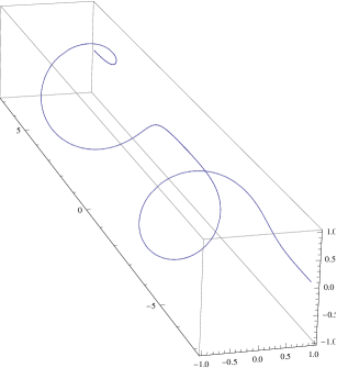
Figure 1: Real and imaginary parts of $v_{1}$ (cf. formula (3.29)) as a function of $x$. Here $\kappa=1$, $\omega=10^{-3}$, $\alpha=1$, $\beta=1+i$, $\gamma=0$.

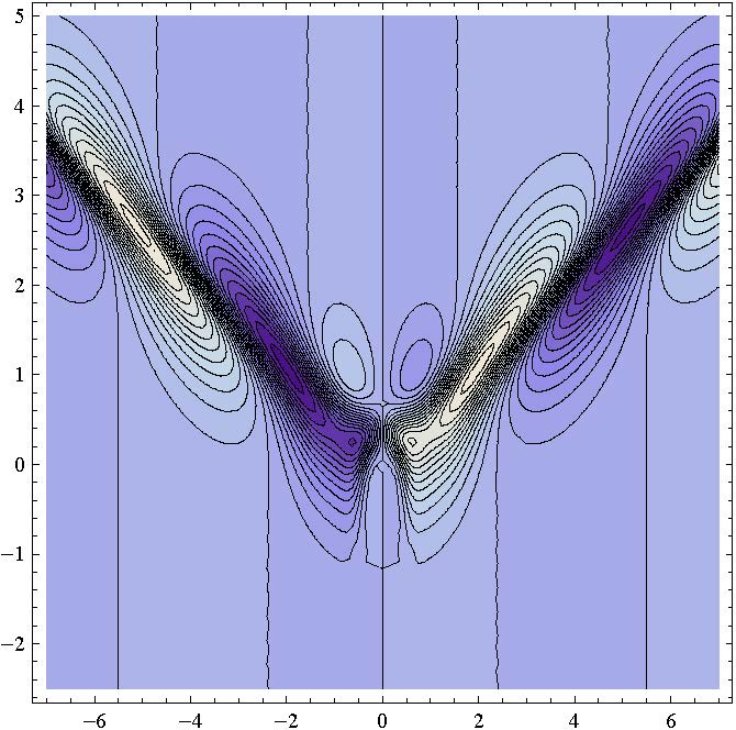
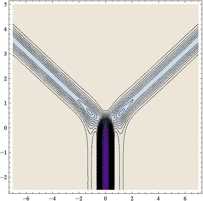
Figure 2: Contour plot of ${\rm Re}\,v_{1}(x,t)$ (left panel) and ${\rm Re}\,u_{1}(x,t)$ (right panel)for a generic soliton solution (see formula 3.30) as a function of $x$ and $t$ where $\alpha=\beta=\gamma=\kappa=\omega=1$.

The function $v_{1}$ can be written in the form $v_{1}=\exp(4i\theta(x))$ where

$$\theta(x)={\rm Arctan}\left(\frac{\kappa\cos(2\omega x+\phi_{\alpha}-\phi_{\beta})}{\omega\cosh(2\kappa x+\ln|\alpha/\beta|)}\right),\qquad\phi_{\alpha}={\rm arg}\,\alpha,\qquad\phi_{\beta}={\rm arg}\,\beta.$$

It is easy to check that $u=0$, $v=\exp(if(x))$ is an exact solution of (2.1) for any differentiable function $f(x)$. It resembles the case of the three-wave equation [49] where one wave of an arbitrary shape is an exact solution of the system and the two other waves are identically zero. A plot of the solution (3.29) is shown on Fig. 1. The solution (3.29) has a simple spectral characterization and an explicitly given analytic fundamental solution of the corresponding linear problem.

Case (ii): $\alpha\neq 0$, $\beta=0$, $\gamma\neq 0$

In this case, from (3.13) it follows that the solution can be written in the form

$$u_{1}=\frac{4i\omega\kappa Q^{*}\exp\{i\omega x+it(\kappa^{2}-\omega^{2})+i(\phi_{\alpha}-\phi_{\gamma})\}}{(\omega-i\kappa)Q^{2}},\qquad v_{1}=1-\frac{8\omega\kappa^{2}}{(\omega-i\kappa)Q^{2}},$$ (3.30)

where

$$Q=2\omega e^{\kappa(x-2\omega t)+\ln|\alpha/\gamma|}+(\omega+i\kappa)e^{-\kappa(x-2\omega t)-\ln|\alpha/\gamma|}.$$

Case (iii): $\alpha=0,\beta\neq 0,\gamma\neq 0$

The solution now can be obtained from the solution in the case (ii), by changing $\alpha\to\beta$ and $x\to-x$.

In the cases (ii) the solution (3.30) is a soliton of width $1/\kappa$ moving with velocity $2\omega$. The corresponding soliton in the case (iii) moves with a velocity $-2\omega$.

In the generic case, when all three constants are non-zero, the solution (3.13) represents a nonlinear interaction of the above described solitons. For $\kappa>0$ it is a decay of unstable time independent soliton from the case (i) into two solitons, corresponding to the cases (ii) and (iii) (see Fig. 2). For $\kappa<0$, the solution is a fusion of two colliding solitons into a stationary one.

Let us now consider the case of imaginary poles, i.e. $\mu=i\kappa$. There exist two essentially different cases.

1. Suppose $p_{0,2}=\gamma=0$. Then from (3.23) it follows that $|p_{0,1}|=|p_{0,3}|$. It suffices to pick up $p_{0,1}=1$ and for the third component we have $p_{0,3}=\exp(i\varphi)$, $\varphi\in{\mathbb{R}}$. In this case the 1-soliton solution is stationary:

$$u(x)=0,\qquad v(x)=\left(\frac{\cosh 2\kappa x+\sinh 2\kappa x\cos\varphi+i(\sigma_{0}-2\kappa x\sin\varphi)}{\cosh 2\kappa x+\sinh 2\kappa x\cos\varphi-i(\sigma_{0}-2\kappa x\sin\varphi)}\right)^{2}.$$

The function $v$ can be presented as

$$v(x)=\exp(4i\,\Xi(x)),\qquad\Xi(x)=\arctan\left(\frac{\sigma_{0}-2\kappa x\sin\varphi}{\cosh 2\kappa x+\sinh 2\kappa x\cos\varphi}\right).$$ (3.31)

A plot of the solution (3.31) is shown on Fig. 3. In particular, when $\varphi=0;\pi$, i.e. $p_{0,1}=\pm p_{0,3}$ we have for the doublet solution:

$$u(x)=0,\qquad v(x)=\left(\frac{e^{\pm 2\kappa x}+i\sigma_{0}}{e^{\pm 2\kappa x}-i\sigma_{0}}\right)^{2}.$$

It is evident that the presence of the constant $\sigma_{0}$ here is essential since otherwise the solution coincides with the vacuum.

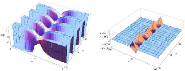
Figure 3: Plots of the phase $\Xi(x)$ (left panel) and ${\rm Im}\,v(x)$ (right panel) for a stationary doublet soliton solution (3.31 ) as a function of $x$ and the phase $\phi$ where $\kappa=\sigma_{0}=1$.

2. Now let us assume $p_{0,2}\neq 0$. For simplicity we fix $p_{0,2}=1$. Then the norms of $p_{0,1}$ and $p_{0,3}$ are interrelated through

$$|p_{0,1}|^{2}-|p_{0,3}|^{2}=1.$$

This is why it proves to be convenient to parametrize them as follows:

$$p_{0,1}=\cosh\theta_{0}e^{i(\varphi_{0}+\tilde{\varphi})},\qquad p_{0,3}=|\sinh\theta_{0}|e^{i(\varphi_{0}-\tilde{\varphi})},\qquad\theta_{0},\varphi_{0},\tilde{\varphi}\in{\mathbb{R}}.$$

The 1-soliton solution reads:

$$u(x,t)=\frac{2\Delta^{*}}{\Delta^{2}}e^{i\left(\kappa^{2}t+\varphi_{0}\right)}\left[\sinh(\kappa x+\theta_{0})\cos\tilde{\varphi}+i\sinh(\kappa x-\theta_{0})\sin\tilde{\varphi}\right],$$

$$v(x,t)=\frac{\Delta^{*}\left(\Delta^{*}-2\right)}{\Delta^{2}}=1+\frac{2(2i\sigma-1)}{\Delta}+\frac{4i\sigma(i\sigma-1)}{\Delta^{2}},$$

where

$$\Delta(x,t)=\cosh^{2}(\kappa x+\theta_{0})\cos^{2}\tilde{\varphi}+\cosh^{2}(\kappa x-\theta_{0})\sin^{2}\tilde{\varphi}-i(\sigma_{0}-2\kappa^{2}t+\kappa x\sinh 2\theta_{0}\sin 2\tilde{\varphi}),$$

$$\sigma(x,t)=\sigma_{0}-2\kappa^{2}t+\kappa x\sinh 2\theta_{0}\sin 2\tilde{\varphi}.$$

The above solution can be significantly simplified if one assumes that $p_{0,3}/p_{0,1}\in{\mathbb{R}}$. In these boundary cases the doublet solution reads:

$$u(x,t)=\frac{2\left(\cosh^{2}(\kappa x+\theta_{0})+i(\sigma_{0}-2\kappa^{2}t)\right)}{\left(\cosh^{2}(\kappa x+\theta_{0})-i(\sigma_{0}-2\kappa^{2}t)\right)^{2}}\,e^{i\left(\kappa^{2}t+\varphi_{0}\right)}\sinh(\kappa x+\theta_{0}),$$

$$v(x,t)=\frac{\left(\cosh^{2}(\kappa x+\theta_{0})+i(\sigma_{0}-2\kappa^{2}t)\right)\left(\cosh^{2}(\kappa x+\theta_{0})+i\sigma_{0}-2-2i\kappa^{2}t\right)}{\left(\cosh^{2}(\kappa x+\theta_{0})-i(\sigma_{0}-2\kappa^{2}t)\right)^{2}}$$ (3.32)

if $p_{0,3}/p_{0,1}>0$ ($\tilde{\varphi}=0$) and

$$u(x,t)=\frac{2\left(\cosh^{2}(\kappa x-\theta_{0})+i(\sigma_{0}-2\kappa^{2}t)\right)}{\left(\cosh^{2}(\kappa x-\theta_{0})-i(\sigma_{0}-2\kappa^{2}t)\right)^{2}}\,e^{i\left(\kappa^{2}t+\varphi_{0}+\pi/2\right)}\sinh(\kappa x-\theta_{0}),$$

$$v(x,t)=\frac{\left(\cosh^{2}(\kappa x-\theta_{0})+i(\sigma_{0}-2\kappa^{2}t)\right)\left(\cosh^{2}(\kappa x-\theta_{0})+i\sigma_{0}-2-2i\kappa^{2}t\right)}{\left(\cosh^{2}(\kappa x-\theta_{0})-i(\sigma_{0}-2\kappa^{2}t)\right)^{2}},$$

when $p_{0,3}/p_{0,1}<0$ ($\tilde{\varphi}=\pi/2$). A plot of the solution (3.32) is depicted on Fig. 4.

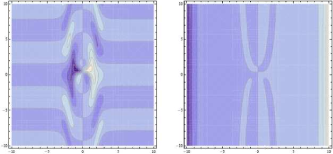
Figure 4: Contour plot of ${\rm Re}\,u(x,t)$ (left panel) and ${\rm Re}\,v(x,t)$ (right panel) for doublet soliton solution of the type (3.32) as a function of $x$ and $t$. Here $\kappa=\sigma_{0}=1$, $\theta_{0}=0$ and $\tilde{\varphi}=0$.

3.3 Multisoliton solutions

As we mentioned above, the dressing procedure can be applied several times consequently. Thus after dressing the $1$-soliton solution one derives a $2$-soliton solution, after dressing the $2$-soliton solution one obtains a $3$-soliton solution and so on. Of course, in doing this one is allowed to apply either of dressing factors (3.8) and (3.17). Therefore the multisoliton solution will be a certain combination of quadruplet and doublet solitons.

Another way of derivation the multisoliton solution consists in using a dressing factor with multiple poles. For example, if one wants to generate $N$ quadruplet solitons one should use a dressing factor in the form:

$$\Phi(x,t,\lambda)=\leavevmode\hbox{\small 1\kern-3.3pt\normalsize 1}+\sum^{N}_{k=1}\lambda\left(\frac{M_{k}(x,t)}{\lambda-\mu_{k}}+\frac{\mathbf{C}M_{k}(x,t)\mathbf{C}}{\lambda+\mu_{k}}\right),$$

which is evidently compatible with the reduction condition (3.3). Due to (3.4) its inverse has the form:

$$\Phi^{-1}(x,t,\lambda)=\leavevmode\hbox{\small 1\kern-3.3pt\normalsize 1}+\sum^{N}_{k=1}\lambda\left(\frac{M^{{\dagger}}_{k}(x,t)}{\lambda-\mu_{k}^{*}}+\frac{\mathbf{C}M^{{\dagger}}_{k}(x,t)\mathbf{C}}{\lambda+\mu_{k}^{*}}\right).$$

In order to determine the residues of $\Phi$ one follows the same steps as in the case of a $2$-poles dressing factor. Firstly, the identity $\Phi\Phi^{-1}=\leavevmode\hbox{\small 1\kern-3.3pt\normalsize 1}$ implies that the residues of $\Phi$ and $\Phi^{-1}$ satisfy certain algebraic relations, namely:

$$M_{k}\left[\leavevmode\hbox{\small 1\kern-3.3pt\normalsize 1}+\sum^{N}_{l=1}\mu_{k}\left(\frac{M^{{\dagger}}_{l}}{\mu_{k}-\mu_{l}^{*}}+\frac{\mathbf{C}M_{l}^{{\dagger}}\mathbf{C}}{\mu_{k}+\mu_{l}^{*}}\right)\right]=0,\qquad k=1,\ldots,N,$$ (3.33)

to ensure vanishing of the residue of $\Phi\Phi^{-1}$ at $\lambda=\mu_{k}$. Of course due to the ${\mathbb{Z}}_{2}$ reductions we will have an additional set of algebraic relations which are obtained from (3.33) by hermitian conjugation.

As discussed before in order to obtain a nontrivial dressing the residues must be degenerate matrices. Thus one introduces the factorization $M_{k}=|\mathbf{n}_{k}\rangle\langle\mathbf{m}_{k}|$ and then reduces (3.33) to a linear system for $|\mathbf{n}_{k}\rangle$

$$|\mathbf{m}_{k}\rangle=\sum^{N}_{l=1}\mathcal{B}_{lk}|\mathbf{n}_{\,l}\rangle,\qquad\mathcal{B}_{lk}:=\mu^{*}_{k}\left(\frac{\langle\mathbf{m}_{\,l}|\mathbf{m}_{k}\rangle}{\mu_{l}-\mu_{k}^{*}}-\frac{\langle\mathbf{m}_{\,l}|\mathbf{C}|\mathbf{m}_{k}\rangle}{\mu_{l}+\mu_{k}^{*}}\mathbf{C}\right).$$

By solving it one can express the vectors $|\mathbf{n}_{l}\rangle$, $l=1,\ldots,N$ through all $|\mathbf{m}_{k}\rangle$ and that way determine the whole dressing factor in terms of $|\mathbf{m}_{k}\rangle$. This step contains the main technical difficulty in the whole scheme.

The vectors $|\mathbf{m}_{k}\rangle$ can be found from the natural requirement of vanishing of the poles in the differential equations (3.14). The result reads

$$|\mathbf{m}_{k}(x,t)\rangle=\psi_{0}(x,t,\mu^{*}_{k})|\mathbf{m}_{k,0}\rangle.$$

Thus we have proved that as in the $2$-poles case the dressing factor is determined if one knows the seed solution $\psi_{0}(x,t,\lambda)$. The quadruplet $N$-soliton solution itself can be derived through the following formula

$$L_{1}^{(1)}=\left(\leavevmode\hbox{\small 1\kern-3.3pt\normalsize 1}+\sum^{N}_{k=1}(M_{k}+\mathbf{C}M_{k}\mathbf{C})\right)L_{1}^{(0)}\left(\leavevmode\hbox{\small 1\kern-3.3pt\normalsize 1}+\sum^{N}_{k=1}(M_{k}+\mathbf{C}M_{k}\mathbf{C})\right)^{{\dagger}}.$$

From all said above it follows that the algorithm for obtaining the $N$-soliton solution can be presented symbolically as follows

$$L_{1}^{(0)}\to(|\mathbf{m}_{1}\rangle,\ldots,|\mathbf{m}_{N}\rangle)\to(|\mathbf{n}_{1}\rangle,\ldots,|\mathbf{n}_{N}\rangle)\to(M_{1},\ldots,M_{N})\to L_{1}^{(1)}.$$

Similarly, one is able to generate a sequence of $N$ doublet solitons by making use of the following factor

$$\Phi(x,t,\lambda)=\leavevmode\hbox{\small 1\kern-3.3pt\normalsize 1}+\sum^{N}_{l=1}\lambda\left(\frac{P_{l}(x,t)}{\lambda-i\kappa_{l}}+\frac{\mathbf{C}P_{l}(x,t)\mathbf{C}}{\lambda+i\kappa_{l}}\right).$$

Following the same steps as in the $1$-soliton case one can convince himself that the vectors $|\mathbf{q}_{\,l}\rangle$ involved in the decomposition $P_{l}=|\mathbf{q}_{l}\rangle\langle\mathbf{p}_{l}|$ satisfy the linear system:

$$\mathbf{C}|\mathbf{p}_{l}\rangle=\sum^{N}_{s=1}\mathcal{D}_{sl}|\mathbf{q}_{s}\rangle,$$

where

$$\mathcal{D}_{ss}:=i\sigma_{s}-\frac{\langle\mathbf{p}_{s}|\mathbf{p}_{s}\rangle}{2}\mathbf{C},\qquad\mathcal{D}_{sl}:=\kappa_{l}\left(\frac{\langle\mathbf{p}_{s}|\mathbf{C}|\mathbf{p}_{l}\rangle}{\kappa_{s}-\kappa_{l}}-\frac{\langle\mathbf{p}_{\,s}|\mathbf{p}_{l}\rangle}{\kappa_{s}+\kappa_{l}}\mathbf{C}\right),\qquad s\neq l.$$

On the other hand the vectors $|\mathbf{p}_{l}\rangle$ and the real functions $\sigma_{l}$ are expressed in terms of the initial solution $\psi_{0}$ and its derivatives with respect to $\lambda$ as follows:

$$|\mathbf{p}_{l}(x,t)\rangle=\psi_{0}(x,t,-i\kappa_{l})|\mathbf{p}_{l,0}\rangle,$$

$$\sigma_{l}(x,t)=-\kappa_{l}\langle\mathbf{p}_{l,0}|\psi^{-1}_{0}(x,t,i\kappa_{l})\dot{\psi}_{0}(x,t,i\kappa_{l})\mathbf{C}|\mathbf{p}_{l,0}\rangle+\sigma_{l,0},$$

where $|\mathbf{p}_{l,0}\rangle$ and $\sigma_{l,0}$ for $l=1,\ldots,N$ are constants of integration to parametrize the solution. The components of $|\mathbf{p}_{l}\rangle$ are not independent but satisfy

$$\langle\mathbf{p}_{l}|\mathbf{C}|\mathbf{p}_{l}\rangle=0\quad\Rightarrow\quad\langle\mathbf{p}_{l,0}|\mathbf{C}|\mathbf{p}_{l,0}\rangle=0.$$

In order to derive doublet $N$-soliton solution one uses:

$$L_{1}^{(1)}=\left(\leavevmode\hbox{\small 1\kern-3.3pt\normalsize 1}+\sum^{N}_{l=1}(P_{l}+\mathbf{C}P_{l}\mathbf{C})\right)L_{1}^{(0)}\left(\leavevmode\hbox{\small 1\kern-3.3pt\normalsize 1}+\sum^{N}_{l=1}(P_{l}+\mathbf{C}P_{l}\mathbf{C})\right)^{{\dagger}}.$$

In this case the diagram which describes the algorithm to obtain the multisoliton solution reads

$$L_{1}^{(0)}\to\{|\mathbf{p}_{\,l}\rangle,\sigma_{l}\}^{N}_{l=1}\to\{|\mathbf{q}_{\,l}\rangle\}^{N}_{l=1}\to\{P_{l}\}^{N}_{l=1}\to L_{1}^{(1)}.$$

It is clear that apart of the ‘pure’ multisolitons discussed above there is a ‘mixed’ type of multisolitons, i.e. multisolitons to contain both species of $1$-soliton solutions. In order to obtain such solution one needs to use a dressing factor possessing both types of poles.

4 Generalized Fourier transform

In this section we aim to develop the generalized Fourier transform interpretation of the inverse scattering method for the Lax operator (2.3). For this to be done we are going to use some basic notions like Wronskian relations, ‘squared solutions’, recursion operators etc. The ‘squared solutions’ also known as adjoint solutions are generalizations of exponential functions in usual Fourier analysis, namely they are a complete system. They occur naturally in Wronskian relations which interrelate the scattering data and the potential $L_{1}(x)$ (as well as their variations) in a form which resembles a scalar product and is called skew-scalar product. The Wronskian relations allows one to express the expansion coefficients of $L_{1}(x)$ and its variation along these generalized exponents in terms of the scattering data and its variations as we shall see later on. Within this framework the role of the operator $id/dx$ whose eigenfunctions are $\exp(ikx)$ is played by the recursion operators. We shall present two substantially different ways of obtaining the recursion operators and compare them.

4.1 Recursion operators and integrable hierarchy

Recursion operators appear in many situations in the theory of integrable systems [2, 21, 42]. Their existence is tightly related to the fact that each integrable NLEE belongs to a whole family of infinite number of integrable NLEEs associated to the same Lax operator $L$. One can also assign to this family a whole infinite set of symmetries and integrals of motion (Hamiltonians). In this subsection we are to derive the recursion operators by analyzing the interrelations between members of the hierarchy of NLEEs. In doing this we are following the ideas in [25, 47].

The hierarchy of integrable NLEEs associated to $L$ is generated through the zero curvature representation which we rewrite in the original Lax form

$$iL_{t}=[L,V].$$

Each choice of $V$ corresponds to an individual member of the hierarchy. Following the ideas in [25] we interrelate two adjacent flows $V$ and $\tilde{V}$ through the equality

$$\tilde{V}(\lambda)=k(\lambda)V(\lambda)+B(\lambda),$$ (4.1)

where $k(\lambda)$ is a scalar function and the remainder $B$ has the structure of the Lax operator $A(\lambda)$

$$B(\lambda)=\lambda B_{1}+\lambda^{2}B_{2}.$$

All quantities above must be invariant with respect to the action of reductions (2.16), (2.17). This is why we pick up $k(\lambda)=\lambda^{2}$ while the operator $B$ obey the condition

$$B^{{\dagger}}(\lambda^{*})=B(\lambda),\qquad\mathbf{C}B(-\lambda)\mathbf{C}=B(\lambda).$$

This means that the coefficients of $B$ are hermitian matrices to fulfill $B_{1}\in\mathfrak{sl}^{1}(3)$, $B_{2}\in\mathfrak{sl}^{0}(3)$.

After substituting (4.1) into the Lax representation one obtains the following relation

$$iL_{\tau}=i\lambda^{2}L_{t}+[L,B],$$ (4.2)

where $\tau$ is the evolution parameter of the flow $\tilde{V}$. Then the recursion operator $\mathcal{R}$ is defined as the mapping

$$L_{1,\tau}=\mathcal{R}L_{1,t}.$$

In order to find it we need to solve (4.2) and thus calculate the remainder $B$.

Since relation (4.2) holds identically with respect to $\lambda$ it splits into the following set of recurrence relations:

$$iL_{1,t}+[L_{1},B_{2}]=0,$$ (4.3)

$$iB_{2,x}+[L_{1},B_{1}]=0,$$ (4.4)

$$L_{1,\tau}-B_{1,x}=0.$$ (4.5)

In accordance with our conventions explained in the Preliminaries (see formulae (2.19)–(2.21)) the coefficients $B_{1}$ and $B_{2}$ have splittings

$$B_{1}=B^{\bot}_{1}+b_{1}L_{1},\qquad\langle B^{\bot}_{1},L_{1}\rangle=0,$$

$$B_{2}=B^{\bot}_{2}+b_{2}L_{2},\qquad\langle B^{\bot}_{2},L_{2}\rangle=0,$$ (4.6)

of terms $B^{\bot}_{1}$ and $B^{\bot}_{2}$ not commuting with $L_{1}$ and their orthogonal complements. After substituting (4.6) into (4.3) it becomes possible to express $B^{\bot}_{2}$ through $L_{1,t}$ as follows:

$$B^{\bot}_{2}=-i\,\mathop{\rm ad}\nolimits^{-1}_{L_{1}}L_{1,t},$$ (4.7)

where $\mathop{\rm ad}\nolimits^{-1}_{L_{1}}$ acts on the orthogonal parts only, i.e. the kernel of $\mathop{\rm ad}\nolimits_{L_{1}}$ is factorized. In this case it can be proven the presentation below holds true

$$\mathop{\rm ad}\nolimits^{-1}_{L_{1}}=\frac{1}{4}\left(5\mathop{\rm ad}\nolimits_{L_{1}}-\mathop{\rm ad}\nolimits^{3}_{L_{1}}\right).$$

The coefficient $b_{2}$ is determined from relation (4.4). Indeed, after plugging (4.6) into (4.4) we get

$$i\partial_{x}B^{\bot}_{2}+ib_{2,x}L_{2}+ib_{2}L_{2,x}+[L_{1},B_{1}]=0.$$ (4.8)

The $L_{1}$-commuting part of (4.8) is separated by taking $\langle\,\cdot\,,L_{2}\rangle$ in both hand sides of the equation to give

$$\frac{2}{3}b_{2,x}+\langle\partial_{x}B^{\bot}_{2},L_{2}\rangle=0\quad\Rightarrow\quad b_{2}=-\frac{3}{2}\partial^{-1}_{x}\langle\partial_{x}B^{\bot}_{2},L_{2}\rangle,$$ (4.9)

where we have denoted by $\partial^{-1}_{x}$ the integral $\int^{x}_{\pm\infty}dy$. On the other hand by projecting (4.4) with $\pi=\mathop{\rm ad}\nolimits^{-1}_{L_{1}}\mathop{\rm ad}\nolimits_{L_{1}}$ one extracts its orthogonal part

$$i\pi\partial_{x}B^{\bot}_{2}+ib_{2}L_{2,x}+[L_{1},B^{\bot}_{1}]=0.$$

Taking into account (4.9) one can find out the following recurrence relation

$$B^{\bot}_{1}=\Lambda_{2}B^{\bot}_{2},\qquad\Lambda_{2}=-i\mathop{\rm ad}\nolimits^{-1}_{L_{1}}\left(\pi\partial_{x}(\cdot)-\frac{3}{2}L_{2,x}\partial^{-1}_{x}\langle\partial_{x}(\cdot),L_{2}\rangle\right).$$ (4.10)

Formally speaking, one should write $\Lambda^{\pm}_{2}$ instead of $\Lambda_{2}$ for the integro-differential operator introduced above since the lower integration limit in $\partial^{-1}_{x}$ differs. This choice of signs, however, is unessential for the considerations in the current subsection and this is why prefer a more simplified notation.

After a similar treatment of (4.5) we obtain

$$2b_{1,x}+\langle\partial_{x}B^{\bot}_{1},L_{1}\rangle=0\quad\Rightarrow\quad b_{1}=-\frac{1}{2}\partial^{-1}_{x}\langle\partial_{x}B^{\bot}_{1},L_{1}\rangle,$$

$$L_{1,\tau}=i\mathop{\rm ad}\nolimits_{L_{1}}\Lambda_{1}B^{\bot}_{1},\qquad\Lambda_{1}=-i\mathop{\rm ad}\nolimits^{-1}_{L_{1}}\left(\pi\partial_{x}(\cdot)-L_{1,x}\frac{1}{2}\partial^{-1}_{x}\langle\partial_{x}(\cdot),L_{1}\rangle\right).$$ (4.11)

Finally combining (4.7), (4.10) and (4.11) one derives

$$L_{1,\tau}=\mathop{\rm ad}\nolimits_{L_{1}}\Lambda_{1}\Lambda_{2}\mathop{\rm ad}\nolimits^{-1}_{L_{1}}L_{1,t}\quad\Rightarrow\quad\mathcal{R}=\mathop{\rm ad}\nolimits_{L_{1}}\Lambda_{1}\Lambda_{2}\mathop{\rm ad}\nolimits^{-1}_{L_{1}}.$$ (4.12)

The recursion operator can be also presented conveniently as a $4\times 4$ matrix to map the column vector $(u,v,u^{*},v^{*})^{T}_{t}$ to the column vector $(u,v,u^{*},v^{*})^{T}_{\tau}$. Then it can be verified that $\mathcal{R}$ obeys the splitting:

$$\mathcal{R}=\pi\mathcal{A}(\mathcal{B}_{\rm{loc}}+\mathcal{B}_{\rm{nonl}})+\mathcal{K}.$$

The factors $\pi$ and $\mathcal{A}$ look as follows

$$\pi=\left(\begin{array}[]{cccc}1-|u|^{2}/2&-uv^{*}/2&-u^{2}/2&-uv/2\\ -u^{*}v/2&1-|v|^{2}/2&-uv/2&-v^{2}/2\\ -(u^{*})^{2}/2&-u^{*}v^{*}/2&1-|u|^{2}/2&-u^{*}v/2\\ -u^{*}v^{*}/2&-(v^{*})^{2}/2&-uv^{*}/2&1-|v|^{2}/2\end{array}\right),$$

$$\mathcal{A}:=i\partial_{x}\left(\begin{array}[]{cccc}0&-v&-u&0\\ -u&0&v&0\\ v^{*}&0&u^{*}&0\\ 0&u^{*}&-v^{*}&0\end{array}\right)\partial_{x}.$$

The matrices

$$\mathcal{B}_{\rm loc}=\frac{i}{4}\left(\begin{array}[]{cccc}0&-4u^{*}&2v(3|v|^{2}-1)&-6u^{*}v^{2}\\ 2v^{*}(1-3|v|^{2})&6u(v^{*})^{2}&0&4u\\ -4u^{*}&0&3u(|v|^{2}-|u|^{2})&-v(1+6|u|^{2})\\ -u^{*}&-v^{*}&0&0\end{array}\right)$$

and

$$\mathcal{B}_{\rm nonl}=-\frac{3i}{4}\begin{pmatrix}2u^{*}v\\ 2uv^{*}\\ |u|^{2}-|v|^{2}\\ -1/3\end{pmatrix}\partial^{-1}_{x}\left[(u^{*}_{x},v^{*}_{x},-u_{x},-v_{x})\right]$$

are a local and a nonlocal part respectively originating from the orthogonal part $B^{\bot}_{2}$ and the $L_{1}$-commuting part $b_{2}L_{2}$. Finally

$$\mathcal{K}=-\frac{1}{2}\begin{pmatrix}u\\ v\\ u^{*}\\ v^{*}\end{pmatrix}_{x}\partial^{-1}_{x}\left[(u^{*},v^{*},u,v)\mathcal{A}(\mathcal{B}_{\rm{loc}}+\mathcal{B}_{\rm{nonl}})\right]$$

is connected with the term $b_{1}L_{1}$ in the splitting of $B_{1}$.

4.2 Wronskian relations and ‘squared solutions’

Wronskian relations [6, 7] provide an important tool for analyzing the relevant class of NLEE and the mapping $\mathfrak{F}:\mathfrak{M}\to\mathfrak{T}$, where $\mathfrak{M}$ is the set of allowed potentials of $L$ (in our case $L_{1}$) and $\mathfrak{T}$ is the minimal set of scattering data.

In deriving them we will need along with the first equation in (2.28) also two other related equations:

$$i\frac{\partial\hat{\chi}}{\partial x}-\lambda\hat{\chi}(x,\lambda)L_{1}(x)=0,\qquad\hat{\chi}(x,\lambda)\equiv\chi^{-1}(x,\lambda),$$

$$i\frac{\partial\delta\chi}{\partial x}+\lambda L_{1}(x)\delta\chi(x,\lambda)+\lambda\delta L_{1}(x)\chi(x,\lambda)=0,$$

where the variation of $\chi(x,\lambda)$ is due to the variation $\delta L_{1}(x)$.

The first type of Wronskian relations interrelates the asymptotics of FAS with $L_{1}$and its powers as shown in the examples below

$$i\left(\hat{\chi}J\chi(x,\lambda)-J\right)\big{|}_{-\infty}^{\infty}=\lambda\int_{-\infty}^{\infty}dx\,\hat{\chi}[L_{1},J]\chi(x,\lambda),$$ (4.13)

$$\hat{\chi}L_{1}(x)\chi(x,\lambda)\big{|}_{-\infty}^{\infty}=\int_{-\infty}^{\infty}dx\,\hat{\chi}L_{1,x}\chi(x,\lambda),$$ (4.14)

$$\hat{\chi}L_{2}(x)\chi(x,\lambda)\big{|}_{-\infty}^{\infty}=\int_{-\infty}^{\infty}dx\,\hat{\chi}L_{2,x}\chi(x,\lambda).$$ (4.15)

We remind the reader that $J=\mathop{\rm diag}\nolimits(1,0,-1)$ and $I=\mathop{\rm diag}\nolimits(1/3,-2/3,1/3)$ are the diagonal forms of (the asymptotics of) $L_{1}$ and $L_{2}=L^{2}_{1}-2\leavevmode\hbox{\small 1\kern-3.3pt\normalsize 1}/3$ respectively, that we introduced at the very beginning in section Preliminaries (see formulae (2.22), (2.23)).

A second class of Wronskian relations connects the variation $\delta\chi(x,\lambda)$ with the variation of $L_{1}$, i.e.

$$\hat{\chi}\delta\chi(x,\lambda)\big{|}_{-\infty}^{\infty}=i\lambda\int_{-\infty}^{\infty}dx\,\hat{\chi}\delta L_{1}\chi(x,\lambda).$$

In the left hand sides of the Wronskian relations are involved the scattering data and its variation while the right hand sides can be viewed as Fourier type integrals. To make this obvious let us take the Killing form of the Wronskian relation (4.13) with a Cartan–Weyl generator $E_{\alpha}$ and use the invariance of the Killing form

$$i\left\langle\hat{\chi}J\chi(x,\lambda)-J,E_{\alpha}\right\rangle\big{|}_{-\infty}^{\infty}=\lambda\int_{-\infty}^{\infty}dx\,\left\langle[L_{1},J],e_{\alpha}(x,\lambda)\right\rangle.$$

The quantities

$$e_{\alpha}(x,\lambda)=\chi E_{\alpha}\hat{\chi}(x,\lambda)$$

introduced above are called ‘squared solutions’. Due to the fact that we have two FAS $\chi^{+}(x,\lambda)$ and $\chi^{-}(x,\lambda)$ we obtain two types of ’squared solutions’ $e^{\pm}_{\alpha}(x,\lambda)$. Similarly, taking the Killing form in (4.14) and (4.15) we find

$$\left\langle\hat{\chi}L_{1}\chi(x,\lambda),E_{\alpha}\right\rangle\big{|}_{-\infty}^{\infty}=\int_{-\infty}^{\infty}dx\,\left\langle L_{1,x},e_{\alpha}(x,\lambda)\right\rangle,$$ (4.16)

$$\left\langle\hat{\chi}L_{2}\chi(x,\lambda),E_{\alpha}\right\rangle\big{|}_{-\infty}^{\infty}=\int_{-\infty}^{\infty}dx\,\left\langle L_{2,x},e_{\alpha}(x,\lambda)\right\rangle,$$ (4.17)

$$\left\langle\hat{\chi}\delta\chi(x,\lambda),E_{\alpha}\right\rangle\big{|}_{-\infty}^{\infty}=i\lambda\int_{-\infty}^{\infty}dx\,\left\langle\delta L_{1},e_{\alpha}(x,\lambda)\right\rangle.$$ (4.18)

We are interested more specifically in variations that are due to the time evolution of $L_{1}(x)$, i.e.

$$\delta L_{1}(x)=L_{1}(x,t+\delta t)-L_{1}(x,t)\simeq\delta t\frac{\partial L_{1}}{\partial t}.$$

Therefore up to first order terms of $\delta t$ we obtain

$$\left\langle\hat{\chi}\chi_{t}(x,\lambda),E_{\alpha}\right\rangle\big{|}_{x=-\infty}^{\infty}=i\lambda\int_{-\infty}^{\infty}dx\,\left\langle L_{1,t},e_{\alpha}(x,\lambda)\right\rangle.$$

Now we can explain why the Wronskian relations are important for analyzing the mapping $\mathfrak{F}:\mathfrak{M}_{L_{1}}\to\mathfrak{T}$. Indeed, taking $\chi(x,\lambda)$ to be a fundamental analytic solution of $L$ we can express the left hand sides of (4.16) and (4.17) (resp. (4.18)) through the Gauss factors $S^{\pm}$, $T^{\mp}$ and $D^{\pm}$ (resp. through the Gauss factors and their variations). The right hand side of (4.16) and (4.17) (resp. (4.18)) can be interpreted as a Fourier-like transformation of the potential $L_{1}(x)$ (resp. of the variation $\delta L_{1}(x)$). As a natural generalization of the usual exponents there appear the ‘squared solutions’. The ‘squared solutions’ are analytic functions of $\lambda$. This fact underlies the proof of their completeness in the space of allowed potentials, as we shall see.

4.3 The skew-scalar product and the mapping $\boldsymbol{\mathfrak{M}_{L_{1}}\to\mathfrak{T}_{j}}$

It is obvious, that only some of the matrix elements of the squared solutions $e_{\alpha}(x,\lambda)$ contribute to the right-hand sides of the Wronskian relations. To make this clearer we will use the ${\mathbb{Z}}_{2}$-grading of the Lie algebra which hints that we should split the squared solutions as in (2.19), namely:

$$e_{\alpha}(x,\lambda)=\mathcal{H}_{\alpha}(x,\lambda)+\mathcal{K}_{\alpha}(x,\lambda),\qquad\mathcal{H}_{\alpha}(x,\lambda)\in\mathfrak{sl}^{0}(3),\qquad\mathcal{K}_{\alpha}(x,\lambda)\in\mathfrak{sl}^{1}(3).$$ (4.19)

In addition, according to (2.20), (2.21) each components $\mathcal{H}_{\alpha}(x,\lambda)$ and $\mathcal{K}_{\alpha}(x,\lambda)$ can be split into

$$\mathcal{H}_{\alpha}(x,\lambda)=H_{\alpha}(x,\lambda)+h_{\alpha}L_{2}(x),\qquad h_{\alpha}=\frac{3}{2}\langle L_{2}(x),\mathcal{H}_{\alpha}(x,\lambda)\rangle,$$

$$\mathcal{K}_{\alpha}(x,\lambda)=K_{\alpha}(x,\lambda)+k_{\alpha}L_{1}(x),\qquad k_{\alpha}=\frac{1}{2}\,\langle L_{1}(x),\mathcal{K}_{\alpha}(x,\lambda)\rangle,$$ (4.20)

where $H_{\alpha}(x,\lambda)$ and $K_{\alpha}(x,\lambda)$ do not commute with $L_{1}(x)$. It is not difficult to realize that only $H_{\alpha}(x,\lambda)$ and $K_{\alpha}(x,\lambda)$ contribute to the right-hand sides of the Wronskian relations.

In what follows we will make use also of the skew-scalar product

$$\big{[}\big{[}X,Y\big{]}\big{]}=\int_{-\infty}^{\infty}dy\,\langle X(y),[L_{1}(y),Y(y)]\rangle,$$

where $X$ and $Y$ are functions with values in $\mathfrak{sl}(3)/\ker{\mathop{\rm ad}\nolimits_{L_{1}}}$ and vanishing for $x\to\pm\infty$.

We will denote the linear space of such functions by $\mathfrak{M}_{L_{1}}$. Note, that we can express the right hand sides of the Wronskian relations using the skew-scalar product:

$$\left\langle\hat{\chi}L_{1}\chi(x,\lambda),E_{\alpha}\right\rangle\big{|}_{x=-\infty}^{\infty}=\big{[}\big{[}e_{\alpha}(x,\lambda),\mathop{\rm ad}\nolimits_{L_{1}}^{-1}L_{1,x}\big{]}\big{]},$$

$$\left\langle\hat{\chi}L_{2}\chi(x,\lambda),E_{\alpha}\right\rangle\big{|}_{x=-\infty}^{\infty}=\big{[}\big{[}e_{\alpha}(x,\lambda),\mathop{\rm ad}\nolimits_{L_{1}}^{-1}L_{2,x}\big{]}\big{]},$$

$$\left\langle\hat{\chi}\delta\chi(x,\lambda),E_{\alpha}\right\rangle\big{|}_{x=-\infty}^{\infty}=i\lambda\big{[}\big{[}e_{\alpha}(x,\lambda),\mathop{\rm ad}\nolimits_{L_{1}}^{-1}\delta L_{1}\big{]}\big{]},$$

$$\left\langle\hat{\chi}\chi_{t}(x,\lambda),E_{\alpha}\right\rangle\big{|}_{x=-\infty}^{\infty}=i\lambda\big{[}\big{[}e_{\alpha}(x,\lambda),\mathop{\rm ad}\nolimits_{L_{1}}^{-1}L_{1,t}\big{]}\big{]}.$$

We should also point out that the skew-scalar product is non-degenerate on $\mathfrak{M}_{L_{1}}$.

We finish this subsection by listing the effective results from the Wronskian relations. Below $\alpha\in\Delta^{+}$:

$$\rho_{\alpha}^{(1),\pm}(\lambda)\equiv\langle\hat{D}^{\pm}\hat{T}^{\mp}JT^{\mp}D^{\pm},E_{\pm\alpha}\rangle=-\big{[}\big{[}\mathop{\rm ad}\nolimits_{L_{1}}^{-1}L_{1,x},K_{\pm\alpha}^{\pm}(x,\lambda)\big{]}\big{]},$$

$$\rho_{\alpha}^{(2),\pm}(\lambda)\equiv\langle\hat{D}^{\pm}\hat{T}^{\mp}IT^{\mp}D^{\pm},E_{\pm\alpha}\rangle=-\big{[}\big{[}\mathop{\rm ad}\nolimits_{L_{1}}^{-1}L_{2,x},H_{\pm\alpha}^{\pm}(x,\lambda)\big{]}\big{]};$$ (4.21)

$$\tau_{\alpha}^{(1),\pm}(\lambda)\equiv\langle\hat{S}^{\pm}JS^{\pm},E_{\mp\alpha}\rangle=\big{[}\big{[}\mathop{\rm ad}\nolimits_{L_{1}}^{-1}L_{1,x},K_{\mp\alpha}^{\pm}(x,\lambda)\big{]}\big{]},$$

$$\tau_{\alpha}^{(2),\pm}(\lambda)\equiv\langle\hat{S}^{\pm}IS^{\pm},E_{\mp\alpha}\rangle=\big{[}\big{[}\mathop{\rm ad}\nolimits_{L_{1}}^{-1}L_{2,x},H_{\mp\alpha}^{\pm}(x,\lambda)\big{]}\big{]};$$ (4.22)

$$\delta^{\prime}\rho_{\alpha}^{\pm}(\lambda)\equiv\langle\hat{D}^{\pm}\hat{T}^{\mp}\delta T^{\mp}D^{\pm},E_{\pm\alpha}\rangle=-i\lambda\big{[}\big{[}\mathop{\rm ad}\nolimits_{L_{1}}^{-1}\delta L_{1},K_{\pm\alpha}^{\pm}(x,\lambda)\big{]}\big{]},$$

$$\delta^{\prime}\tau_{\alpha}^{\pm}(\lambda)\equiv\langle\hat{S}^{\pm}\delta S^{\pm},E_{\mp\alpha}\rangle=i\lambda\big{[}\big{[}\mathop{\rm ad}\nolimits_{L_{1}}^{-1}\delta L_{1},K_{\mp\alpha}^{\pm}(x,\lambda)\big{]}\big{]}.$$ (4.23)

In deriving the above formulae, besides the splitting (4.19) we also used the fact that $\mathop{\rm ad}\nolimits_{L_{1}}^{-1}\delta L_{1},\mathop{\rm ad}\nolimits_{L_{1}}^{-1}L_{1,x}\in\mathfrak{sl}^{0}(3)$ and $\mathop{\rm ad}\nolimits_{L_{1}}^{-1}L_{2,x}\in\mathfrak{sl}^{1}(3)$.

The quantities $\rho_{\alpha}^{(k),\pm}$, $\tau_{\alpha}^{(k),\pm}$, $k=1,2$, can be viewed as reflection coefficients. These formulae provide the basis in the analysis of the mapping $\mathfrak{M}_{L_{1}}\to\mathfrak{T}_{k}$, $k=1,2$. Indeed $L_{1,x}\in\mathfrak{M}_{L_{1}}$, while the sets of coefficients

$$\mathfrak{T}_{1}\equiv\mathfrak{T}_{1}^{(1)}\cup\mathfrak{T}_{1}^{(2)},\qquad\mathfrak{T}_{1}^{(k)}\equiv\big{\{}\tau_{\alpha}^{(k),\pm}(\lambda),\ \lambda\in{\mathbb{R}},\ \alpha>0\big{\}},$$

$$\mathfrak{T}_{2}\equiv\mathfrak{T}_{2}^{(1)}\cup\mathfrak{T}_{2}^{(2)},\qquad\mathfrak{T}_{2}^{(k)}\equiv\big{\{}\rho_{\alpha}^{(k),\pm}(\lambda),\ \lambda\in{\mathbb{R}},\ \alpha>0\big{\}}$$

completed with additional sets characterizing the discrete spectrum of $L$ are candidates for the minimal sets of scattering data of the Lax operator.

The above considerations show, that following [2] we can treat the ‘squared solutions’ as generalized exponentials. Therefore the mapping $\mathfrak{M}_{L_{!}}$ can be viewed as a generalized Fourier transform.

Of course, the justifications of the above statements must be based on a proof of the completeness relation for the ‘squared solutions’ which will be presented in the next section.

4.4 Recursion operators – an alternative approach

Our goal in this subsection is to present an alternative definition of the recursion operators. We introduce them as operators $\Lambda^{\pm}$ whose eigenfunctions are the ‘squared solutions’. More precisely, we shall see that the following equality holds:

$$\Lambda^{\pm}K_{\alpha}^{\pm}(x,\lambda)=\lambda^{2}K_{\alpha}^{\pm}(x,\lambda).$$

Our consideration starts from analysis of the equation

$$i\partial_{x}e_{\alpha}+\lambda[L_{1}(x),e_{\alpha}(x,\lambda)]=0$$

satisfied by each of the ‘squared solutions’. We have omitted the superscript $\pm$ in the notation of the squared solutions since it does not play a significant role in most of our further considerations. We shall use it again at the end of subsection when it will become essential.

Due to the grading condition (2.18) the components $\mathcal{H}_{\alpha}$ and $\mathcal{K}_{\alpha}$ are interrelated through the system

$$i\partial_{x}\mathcal{H}_{\alpha}+\lambda[L_{1}(x),\mathcal{K}_{\alpha}(x,\lambda)]=0,\qquad i\partial_{x}\mathcal{K}_{\alpha}+\lambda[L_{1}(x),\mathcal{H}_{\alpha}(x,\lambda)]=0.$$ (4.24)

After we extract terms proportional to $L_{1}$ from the above equations we obtain

$$\langle L_{2},\partial_{x}H_{\alpha}\rangle+\partial_{x}h_{\alpha}=0\quad\Rightarrow\quad h_{\alpha}=h_{\alpha,0}-\frac{3}{2}\partial_{x}^{-1}\langle L_{2},\partial_{x}H_{\alpha}\rangle,$$

$$\langle L_{1},\partial_{x}K_{\alpha}\rangle+\partial_{x}k_{\alpha}=0\quad\Rightarrow\quad k_{\alpha}=k_{\alpha,0}-\frac{1}{2}\partial_{x}^{-1}\langle L_{1},\partial_{x}K_{\alpha}\rangle,$$

where $h_{\alpha,0}$ and $k_{\alpha,0}$ are some integration constants. On the other hand the orthogonal part of (4.24) reads:

$$i\pi\partial_{x}H_{\alpha}+ih_{\alpha}L_{2,x}=-\lambda[L_{1}(x),K_{\alpha}],\qquad i\pi\partial_{x}K_{\alpha}+i\,k_{\alpha}L_{1,x}=-\lambda[L_{1}(x),H_{\alpha}].$$

After substituting $h_{\alpha}$ and $k_{\alpha}$ in the equations above we get

$$\Lambda_{1}K_{\alpha}=\lambda H_{\alpha}-k_{\alpha,0}\Lambda_{2}L_{2},$$ (4.25)

$$\Lambda_{2}H_{\alpha}=\lambda K_{\alpha}-h_{\alpha,0}\Lambda_{1}L_{1},$$ (4.26)

where the operators $\Lambda_{2}$ and $\Lambda_{1}$ are given in (4.10) and (4.11) respectively. This is the right place to mention that remarkably the operators $\Lambda_{1,2}$ are invertible. Indeed, they admit the factorization

$$\Lambda_{1}X=-i\mathop{\rm ad}\nolimits_{L_{1}}^{-1}\mathcal{J}_{1}\partial_{x}X,\qquad\mathcal{J}_{1}X=X-\frac{1}{2}L_{1,x}\partial_{x}^{-1}\langle L_{1},X\rangle,$$

$$\Lambda_{2}Y=-i\mathop{\rm ad}\nolimits_{L_{1}}^{-1}\mathcal{J}_{2}\partial_{x}Y,\qquad\mathcal{J}_{2}Y=X-\frac{3}{2}L_{2,x}\partial_{x}^{-1}\langle L_{2},X\rangle.$$

It is not hard to see that the operators $\mathcal{J}_{1}$ and $\mathcal{J}_{2}$ can be inverted as follows

$$\mathcal{J}_{1}^{-1}X=X+\frac{1}{2}L_{1,x}\partial_{x}^{-1}\langle L_{1},X\rangle,\qquad\mathcal{J}_{2}^{-1}Y=X+\frac{3}{2}L_{2,x}\partial_{x}^{-1}\langle L_{2},X\rangle.$$

Therefore $\Lambda_{1}$ and $\Lambda_{2}$ are invertible as well, namely

$$\Lambda_{1}^{-1}X=i\partial_{x}^{-1}\mathcal{J}_{1}^{-1}\mathop{\rm ad}\nolimits_{L_{1}}X,\qquad\Lambda_{2}^{-1}X=i\partial_{x}^{-1}\mathcal{J}_{2}^{-1}\mathop{\rm ad}\nolimits_{L_{1}}Y.$$

Let us apply $\Lambda_{2}$ to (4.25) and $\Lambda_{1}$ to (4.26). After restoring the index notation where needed the result reads:

$$\Lambda^{\pm}_{2}\Lambda^{\pm}_{1}K_{\alpha}^{\pm}=\lambda^{2}K_{\alpha}^{\pm}-\lambda h_{\alpha,0}\Lambda^{\pm}_{1}L_{1}-k_{\alpha,0}\Lambda^{\pm}_{2}\Lambda^{\pm}_{2}L_{2},$$

$$\Lambda^{\pm}_{1}\Lambda^{\pm}_{2}H_{\alpha}^{\pm}=\lambda^{2}H_{\alpha}^{\pm}-\lambda k_{\alpha,0}\Lambda^{\pm}_{2}L_{2}-h_{\alpha,0}\Lambda^{\pm}_{1}\Lambda^{\pm}_{2}L_{2}.$$

This is the right place to remind the reader that the constants $h_{\alpha,0}$ and $k_{\alpha,0}$ are determined by the asymptotic of the relevant ‘squared solution’ for $x\to\infty$ (or for $x\to-\infty$), depending on the proper definition of the recursion operator. More detailed analysis shows that for each $\Lambda_{1}^{\pm}$ and $\Lambda_{2}^{\pm}$ there exist certain roots for which the constants $k_{\alpha,0}$ and $h_{\alpha,0}$ vanish. More specifically the following equalities holds:

$$\Lambda_{1}^{+}K^{\pm}_{\mp\alpha}(x,\lambda)=\lambda H^{\pm}_{\mp\alpha}(x,\lambda),\qquad\Lambda_{1}^{-}K^{\pm}_{\pm\alpha}(x,\lambda)=\lambda H^{\pm}_{\pm\alpha}(x,\lambda),$$

$$\Lambda_{2}^{+}H^{\pm}_{\mp\alpha}(x,\lambda)=\lambda K^{\pm}_{\mp\alpha}(x,\lambda),\qquad\Lambda_{2}^{-}K^{\pm}_{\pm\alpha}(x,\lambda)=\lambda K^{\pm}_{\pm\alpha}(x,\lambda)$$

for all roots $\alpha>0$ and therefore:

$$\Lambda_{2}^{+}\Lambda_{1}^{+}K^{\pm}_{\mp\alpha}(x,\lambda)=\lambda^{2}K^{\pm}_{\mp\alpha}(x,\lambda),\qquad\Lambda_{2}^{-}\Lambda_{1}^{-}K^{\pm}_{\pm\alpha}(x,\lambda)=\lambda^{2}K^{\pm}_{\pm\alpha}(x,\lambda),$$

$$\Lambda_{1}^{+}\Lambda_{2}^{+}H^{\pm}_{\mp\alpha}(x,\lambda)=\lambda^{2}H^{\pm}_{\mp\alpha}(x,\lambda),\qquad\Lambda_{1}^{-}\Lambda_{2}^{-}H^{\pm}_{\pm\alpha}(x,\lambda)=\lambda^{2}H^{\pm}_{\pm\alpha}(x,\lambda).$$

The operator $\Lambda^{\pm}$ introduced as

$$\Lambda^{\pm}X=\Lambda^{\pm}_{1}\Lambda^{\pm}_{2}X,\quad X\in\mathfrak{sl}^{0}(3),\qquad\tilde{\Lambda}Y=\Lambda^{\pm}_{2}\Lambda^{\pm}_{1}Y,\quad Y\in\mathfrak{sl}^{1}(3)$$ (4.27)

is the recursion operator we have been looking for. If we compare (4.27) and (4.12) we can conclude that both approaches lead to compatible results which coincide up to some conjugation by $\mathop{\rm ad}\nolimits_{L_{1}}$.

5 Spectral theory of the recursion operators

5.1 Asymptotics of the fundamental analytic solution

For performing the contour integration, in order to derive the completeness relations for the squared solutions, one needs the asymptotics of the squared solutions for $|\lambda|\to\infty$. The starting point here is the asymptotic expansion of the FAS for $\lambda\to\infty$:

$$\chi_{\rm as}(x,\lambda)=\leavevmode\hbox{\small 1\kern-3.3pt\normalsize 1}+\sum_{k=1}^{\infty}\chi_{k}(x)\lambda^{-k}.$$

Introduce:

$$\tilde{\chi}_{\rm as}(x,\lambda)=g^{-1}(x)\chi_{\rm as}(x,\lambda)e^{iJ\lambda x},$$

which satisfy:

$$i\frac{d\tilde{\chi}_{\rm as}}{dx}+ig^{-1}g_{x}\tilde{\chi}_{\rm as}(x,\lambda)+\lambda[J,\tilde{\chi}_{\rm as}(x,\lambda)]=0.$$ (5.1)

Together with properly chosen asymptotic conditions $\tilde{\chi}_{\rm as}(x,\lambda)$ the last equation will provide the asymptotics of the fundamental analytic solution. Therefore it will allow an asymptotic expansion of the form:

$$\tilde{\chi}_{\rm as}(x,\lambda)=\sum_{s=0}^{\infty}\lambda^{-s}\tilde{\chi}_{k,\rm as}(x).$$

This will lead to a recurrent relations for the expansion coefficients $\tilde{\chi}_{k,\rm as}(x)$. Inserting this expansion into equation (5.1) for the first two coefficients of $\tilde{\chi}_{\rm as}(x,\lambda)$ we get:

$$[J,\tilde{\chi}_{0,\rm as}(x)]=0,$$ (5.2)

$$i\frac{d\tilde{\chi}_{0,\rm as}}{dx}-ig^{-1}_{x}g\tilde{\chi}_{0,\rm as}(x)+[J,\tilde{\chi}_{1,\rm as}(x)]=0,$$ (5.3)

$$i\frac{d\tilde{\chi}_{1,\rm as}}{dx}-ig^{-1}_{x}g\tilde{\chi}_{1,\rm as}(x)+[J,\tilde{\chi}_{2,\rm as}(x)]=0.$$

From (5.2) it follows that $\tilde{\chi}_{0,\rm as}(x)$ must be a diagonal matrix and using the diagonal part of (5.3) one can derive it in an explicit form:

$$\tilde{\chi}_{0,\rm as}(x)=\mathop{\rm diag}\nolimits\big{(}e^{\rho(x)},e^{-2\rho(x)},e^{\rho(x)}\big{)},\qquad\rho(x)=\frac{1}{2}\int_{\pm\infty}^{x}dy(u^{*}u_{y}+v^{*}v_{y}),$$ (5.4)

and for the off-diagonal part of $\tilde{\chi}^{\rm f}_{1,\rm as}(x)$ we have (see equation (2.27)):

$$\tilde{\chi}^{\rm f}_{1,\rm as}(x)=\frac{i}{2}\left(\!\!\begin{array}[]{c@{\,\,\,}c@{\,\,\,}c}0&\sqrt{2}(uv_{x}-vu_{x})e^{-\rho(x)}&(u^{*}u_{x}+v^{*}v_{x})e^{\rho(x)}/2\\ \sqrt{2}(u^{*}v^{*}_{x}-v^{*}u^{*}_{x})e^{\rho(x)}&0&-\sqrt{2}(u^{*}v^{*}_{x}-v^{*}u^{*}_{x})e^{2\rho(x)}\\ -(u^{*}u_{x}+v^{*}v_{x})e^{\rho(x)}/2&\sqrt{2}(vu_{x}-uv_{x})e^{-2\rho(x)}&0\end{array}\!\!\right).$$

As a result the asymptotic behavior of $\chi(x,\lambda)$ for $\lambda\to\infty$ is given by:

$$\chi(x,\lambda)\mathop{\simeq}\limits_{\lambda\to\infty}g(x)\left(\tilde{\chi}_{0,\rm as}(x)+\frac{1}{\lambda}\tilde{\chi}_{1,\rm as}(x)+\cdots\right)e^{-iJ\lambda x}.$$ (5.5)

Note, that the fundamental analytic solution $\chi^{\pm}$ does not allow a canonical normalization for $|\lambda|\to\infty$. This difficulty can be overcome by applying a suitable gauge transformation.

Using the asymptotic behavior (5.5) of the FAS, one can derive the asymptotics of the squared solutions $e_{\alpha}(x,\lambda)=(\chi(x,\lambda)E_{\alpha}\chi^{-1}(x,\lambda))^{\rm f}$. Skipping the details:

$$e^{\pm}_{\alpha}(x,\lambda)\mathop{\simeq}\limits_{\lambda\to\infty}e^{i(J,\alpha)\lambda x}g(x)\tilde{\chi}_{\rm as}(x)E_{\alpha}\tilde{\chi}_{\rm as}^{-1}(x)g^{-1}(x)$$

$$\phantom{e^{\pm}_{\alpha}(x,\lambda)}{}=e^{i(J,\alpha)\lambda x+3\rho(x)(I,\alpha)}g(x)\left(E_{\alpha}+\mathcal{O}\big{(}\lambda^{-1}\big{)}\right)g^{-1}(x).$$

5.2 Completeness of squared solutions

Below we will derive the completeness relation for the ‘squared solutions’ for a class of potentials $L_{1}(x)$ of the Lax operator $L$ which for every fixed value of $t$ satisfy the following conditions:

C1)

$L_{1}(x)-L_{1,\pm}$ is complex valued function of Schwartz type, i.e. it is infinitely smooth function of $x$ falling off for $|x|\to\infty$ faster than any power of $x$;

C2)

$L_{1}(x)$ is such that the corresponding functions $m_{1}^{\pm}(\lambda)$ and $m_{2}^{\pm}(\lambda)$ have at most finite number of simple zeroes. For simplicity we assume also that $m_{1}^{+}(\lambda)$ and $m_{2}^{+}(\lambda)$ (resp. $m_{1}^{-}(\lambda)$ and $m_{2}^{-}(\lambda)$) have no common zeroes;

C3)

the corresponding functions $m_{1}^{\pm}(\lambda)$ and $m_{2}^{\pm}(\lambda)$ have no zeroes on the real axis of the complex $\lambda$-plane.

Remark 5.1.

It is well known that the zeroes of the functions $m_{1}^{\pm}(\lambda)$ and $m_{2}^{\pm}(\lambda)$ determine the discrete spectrum of $L$. The proof of this fact comes out of the scope of the present paper. For other classes of Lax operators it is well known, see e.g. [12, 21].

Below for definiteness we introduce notations for the discrete eigenvalues. As we already mentioned, due to the two ${\mathbb{Z}}_{2}$-reductions, they are of two types. Let there be $N_{1}$ discrete eigenvalues of generic type which come in quadruplets (see Fig. 5). We will denote by $\lambda_{1}^{+},\lambda_{2}^{+},\dots,$ $\lambda_{N_{1}}^{+}$ those of them that are in the first quadrant, i.e. $0<\arg\lambda_{k}^{+}<\pi/2$, $1\leq k\leq N_{1}$. The eigenvalues $\lambda_{N_{1}+k}^{+}=-(\lambda_{k}^{+})^{*}$ belong also to ${\mathbb{C}}_{+}$ but are in the second quadrant. Besides we have also $\lambda_{j}^{-}=(\lambda_{j}^{+})^{*}$, $j=1,\dots,2N_{1}$ which lie in ${\mathbb{C}}_{-}$. The second type of discrete eigenvalues are purely imaginary, i.e. $\lambda_{2N_{1}+a}^{+}=i\nu_{a}$, $a=1,\dots,N_{2}$; obviously $\lambda_{2N_{1}+a}^{-}=-i\nu_{a}$. Therefore the Lax operator $L$ will have $4N_{1}+2N_{2}$ discrete eigenvalues.

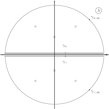
Figure 5: The bold line defines the continuous spectrum of $L$, the regular lines show the integration contours $\gamma_{\pm}$; by $\gamma_{\pm,\infty}$ we denote the ‘infinite’ semi-circles. By $\circ$ we denote the discrete eigenvalues relevant for one generic soliton which come in quadruplets $\pm\lambda_{j}^{\pm}$; the second type of solitons correspond to purely imaginary pairs of discrete eigenvalues $\pm i\nu_{a}$ denoted by $\times.$

Consider the Green function:

$$G^{\pm}(x,y,\lambda)=G_{1}^{\pm}(x,y,\lambda)\theta(y-x)-G_{2}^{\pm}(x,y,\lambda)\theta(x-y),$$ (5.6)

$$G_{1}^{\pm}(x,y,\lambda)=\sum_{\alpha\in\Delta^{+}}e_{\pm\alpha}^{\pm}(x,\lambda)\otimes e_{\mp\alpha}^{\pm}(y,\lambda),$$ (5.7)

$$G_{2}^{\pm}(x,y,\lambda)=\sum_{\alpha\in\Delta^{-}}e_{\pm\alpha}^{-}(x,\lambda)\otimes e_{\mp\alpha}^{-}(y,\lambda)+\sum_{j=1}^{r}h_{j}^{\pm}(x,\lambda)\otimes h_{j}^{\pm}(y,\lambda),$$ (5.8)

$$h_{j}^{\pm}(x,\lambda)=\chi^{\pm}(x,\lambda)H_{j}\hat{\chi}^{\pm}(x,\lambda).$$ (5.9)

In order to derive the completeness relations for the squared solutions, one needs to apply a contour integration to the integral:

$$\mathcal{J}_{G}(x,y)=\frac{1}{2\pi i}\oint_{\gamma_{+}}d\lambda\,G^{+}(x,y,\lambda)-\frac{1}{2\pi i}\oint_{\gamma_{-}}d\lambda\,G^{-}(x,y,\lambda),$$

where the integration contours $\gamma_{\pm}={\mathbb{R}}\cup\gamma_{\pm,\infty}$ are shown on Fig. 5.

Let us recall that the Lax operator $L$ has two types of discrete eigenvalues whose number is $4N_{1}+2N_{2}$; the first type correspond to generic solitons and come in quadruplets $\pm\lambda_{j}^{\pm}$; the second type correspond to purely imaginary pairs of discrete eigenvalues $\pm i\nu_{a}$. Thus according to Cauchy’s residuum theorem

$$\mathcal{J}_{G}(x,y)=\sum_{k=1}^{2N_{1}+N_{2}}\left(\mathop{\rm Res}\limits_{\lambda=\lambda_{k}^{+}}\,G^{+}(x,y,\lambda)+\mathop{\rm Res}\limits_{\lambda=\lambda_{k}^{-}}\,G^{-}(x,y,\lambda)\right),$$

presuming that the radii of the ‘infinite’ semicircles are large enough so that all discrete eigenvalues are inside the contours $\gamma_{\pm}$. Condition C3 above ensures that $G^{\pm}(x,y,\lambda)$ has no poles on the continuous spectrum.

Next we integrate along the contours:

$$\mathcal{J}_{G}(x,y)=\frac{1}{2\pi i}\int_{-\infty}^{\infty}d\lambda\,(G^{+}(x,y,\lambda)-G^{-}(x,y,\lambda))$$

$$\hphantom{\mathcal{J}_{G}(x,y)=}{}+\frac{1}{2\pi i}\oint_{\gamma_{+,\infty}}d\lambda\,G^{+}_{\rm as}(x,y,\lambda)-\frac{1}{2\pi i}\oint_{\gamma_{-,\infty}}d\lambda\,G^{-}_{\rm as}(x,y,\lambda).$$

In order to calculate the integrals over $\gamma_{\pm,\infty}$ it is enough to use the asymptotic behavior of the Green function for $\lambda\to\infty$. From equations (5.4) and (5.5) we have:

$$G^{\pm}_{1,\rm as}(x,t,\lambda)\mathop{\simeq}\limits_{\lambda\to\infty}\sum_{\alpha\in\Delta_{+}}e^{i(J,\alpha)\lambda(x-y)+3(\rho(x)-\rho(y))(I,\alpha)}$$

$$\hphantom{G^{\pm}_{1,\rm as}(x,t,\lambda)\mathop{\simeq}\limits_{\lambda\to\infty}}{}\times\left(g(x)\otimes g(y)\right)\left(E_{\pm\alpha}\otimes E_{\mp\alpha}+\mathcal{O}(\lambda^{-1})\right)(g^{-1}(x)\otimes g^{-1}(y))$$

and

$$G^{\pm}_{2,\rm as}(x,t,\lambda)\mathop{\simeq}\limits_{\lambda\to\infty}\sum_{j=1}^{r}(g(x)\otimes g(y))\left(H_{j}\otimes H_{j}^{\vee}+\mathcal{O}(\lambda^{-1})\right)(g^{-1}(x)\otimes g^{-1}(y))$$

$$+\sum_{\alpha\in\Delta_{0}\cup\Delta_{1}^{-}}e^{i(J,\alpha)\lambda(x-y)+3(\rho(x)-\rho(y))(I,\alpha)}(g(x)\otimes g(y))\left(E_{\pm\alpha}\otimes E_{\mp\alpha}+\mathcal{O}(\lambda^{-1})\right)(\hat{g}(x)\otimes\hat{g}(y)).$$

As a result we get:

$$\frac{1}{2\pi i}\oint_{\gamma_{+,\infty}}d\lambda\,G^{+}_{\rm as}(x,y,\lambda)-\frac{1}{2\pi i}\oint_{\gamma_{-,\infty}}d\lambda\,G^{-}_{\rm as}(x,y,\lambda)$$

$$\qquad{}=\delta(x-y)\left(g(x)\otimes g(y)\right)\sum_{\alpha\in\Delta_{+}}\left(E_{\alpha}\otimes E_{-\alpha}-E_{-\alpha}\otimes E_{\alpha}\right)\left(\hat{g}(x)\otimes\hat{g}(y)\right).$$

The next step is to simplify the integral along the continuous spectrum; namely we will calculate the jump of the Green function with the result:

$$G^{+}(x,y,\lambda)-G^{-}(x,y,\lambda)=G^{+}_{1}(x,y,\lambda)-G^{-}_{1}(x,y,\lambda)$$

$$\phantom{G^{+}(x,y,\lambda)-G^{-}(x,y,\lambda)}{}=\sum_{\alpha\in\Delta_{+}}\left(e^{+}_{\alpha}(x,\lambda)\otimes e^{+}_{-\alpha}(x,\lambda)-e^{-}_{-\alpha}(x,\lambda)\otimes e^{-}_{\alpha}(x,\lambda)\right).$$

The proof of this fact goes as follows. From the expression for the Green function (equations (5.6)–(5.9)) and using the relation $\theta(x-y)+\theta(y-x)=1$ we easily get:

$$G^{+}(x,y,\lambda)-G^{-}(x,y,\lambda)=G^{+}_{1}(x,y,\lambda)-G^{-}_{1}(x,y,\lambda)$$

$$\qquad{}-\theta(x-y)(G_{1}^{+}(x,y,\lambda)+G_{2}^{+}(x,y,\lambda)-G^{-}_{1}(x,y,\lambda)-G^{-}_{2}(x,y,\lambda)),$$

so it will be enough to prove that the coefficient in front of $\theta(x-y)$ vanishes. Indeed, we have:

$$G_{1}^{+}(x,y,\lambda)+G_{2}^{+}(x,y,\lambda)-G^{-}_{1}(x,y,\lambda)-G^{-}_{2}(x,y,\lambda)$$

$$\qquad{}=(\chi^{+}(x,\lambda)\otimes\chi^{+}(y,\lambda))\Pi_{2}(\hat{\chi}^{+}(x,\lambda)\otimes\hat{\chi}^{+}(y,\lambda))$$

$$\qquad\quad{}-(\chi^{-}(x,\lambda)\otimes\chi^{-}(y,\lambda))\Pi_{2}(\hat{\chi}^{-}(x,\lambda)\otimes\hat{\chi}^{-}(y,\lambda)).$$

Here

$$\Pi_{2}=\sum_{\alpha\in\Delta_{+}}(E_{\alpha}\otimes E_{-\alpha}+E_{-\alpha}\otimes E_{\alpha})+\sum_{k=1}^{2}\frac{H_{k}\otimes H_{k}}{\langle H_{k},H_{k}\rangle}$$

and $H_{1}=J$, $H_{2}=J_{4}$. Note that $\Pi_{2}$ is the second Casimir endomorphism for the algebra $sl(3)$. It remains to use equation (2.51) and the basic property of $\Pi_{2}$ that states:

$$(G(\lambda)\otimes G(\lambda))\Pi_{2}(\hat{G}(\lambda)\otimes\hat{G}(\lambda))=\Pi_{2},$$

for any element $G(\lambda)$ of the corresponding group $SL(3)$.

We evaluate the contribution from the discrete spectrum assuming that the squared solutions $e^{\pm}_{\alpha}(x,\lambda)$ have at most simple poles at the points of the discrete spectrum. Therefore in the vicinity of the eigenvalues $\lambda_{k}^{\pm}$ we use the following expansions of the ‘squared solutions’:

$$e^{\pm}_{\alpha}(x,\lambda)=(\lambda-\lambda_{k}^{\pm})^{p_{\alpha}}\left(\frac{e^{\pm}_{\alpha,k}}{\lambda-\lambda_{k}^{\pm}}+\dot{e}^{\pm}_{\alpha,k}\right),$$

where $p_{\alpha}$ are integers and $p_{\alpha}=-p_{-\alpha}$. Thus we obtain:

$$\mathop{\rm Res}\limits_{\lambda=\lambda_{k}^{+}}\,G^{+}(x,y,\lambda)=\sum_{\alpha\in\Delta_{+}}\big{(}e^{\pm}_{\alpha,k}\otimes\dot{e}^{\pm}_{-\alpha,k}+\dot{e}^{\pm}_{\alpha,k}\otimes e^{\pm}_{-\alpha,k}\big{)}.$$

Therefore the completeness relations takes the form:

$$\delta(x-y)\left(g(x)\otimes g(y)\right)\Pi_{0}\left(\hat{g}(x)\otimes\hat{g}(y)\right)$$

$$\qquad{}=\frac{i}{2\pi}\int_{-\infty}^{\infty}d\lambda\;\sum_{\alpha\in\Delta_{+}}\left(e^{+}_{\alpha}(x,\lambda)\otimes e^{+}_{-\alpha}(x,\lambda)-e^{-}_{-\alpha}(x,\lambda)\otimes e^{-}_{\alpha}(x,\lambda)\right)$$

$$\qquad\quad{}+\sum_{k=1}^{2N_{1}+N_{2}}\sum_{\alpha\in\Delta_{+}}\big{(}e^{+}_{\alpha,k}(x)\otimes\dot{e}^{+}_{-\alpha,k}(y)+\dot{e}^{+}_{\alpha,k}(x)\otimes e^{+}_{-\alpha,k}(y)$$

$$\qquad\quad{}+e^{-}_{-\alpha,k}(x)\otimes\dot{e}^{-}_{\alpha,k}(y)+\dot{e}^{-}_{-\alpha,k}(x)\otimes e^{-}_{\alpha,k}(y)\big{)},$$ (5.10)

where

$$\Pi_{0}=\sum_{\alpha\in\Delta_{+}}\frac{E_{\alpha}\otimes E_{-\alpha}-E_{-\alpha}\otimes E_{\alpha}}{(\alpha,J)}$$

and

$$e^{\pm}_{\alpha,k}=e^{-}_{\alpha}(x,\lambda_{k}^{\pm}),\qquad\dot{e}^{\pm}_{\alpha,k}=\left.\frac{\partial e^{\pm}_{\alpha}(x,\lambda)}{\partial\lambda}\right|_{\lambda=\lambda_{k}^{\pm}}.$$

5.3 Expansion over the ‘squared solutions’

Using the completeness relations of the squared solutions, one can expand any generic element $F(x)$ of the phase space $\mathcal{M}$ over the complete sets of squared solutions. We remind that $F(x)$ is a generic element of $\mathcal{M}$ if it tends fast enough to zero for $|x|\to\infty$ and is ‘perpendicular’, i.e.

$$\langle F(x),L_{1}\rangle=\langle F(x),L_{2}\rangle=0.$$

It can be parametrized as follows:

$$F(x)=g(x)\sum_{\alpha\in\Delta_{+}\cup\Delta_{-}}F_{\alpha}(x)E_{\alpha}g(x).$$

Let us now multiply both sides of the completeness relation (5.10) by $\leavevmode\hbox{\small 1\kern-3.3pt\normalsize 1}\otimes[L_{1}(y),F(y)]$ on the right, take the Killing form of the second factors in the tensor product and integrate over $y$. In the left hand side after some manipulations we get:

$$\int_{-\infty}^{\infty}dy\;\left\langle(g(x)\otimes g(y))\Pi_{0}(\hat{g}(x)\otimes\hat{g}(y)),\leavevmode\hbox{\small 1\kern-3.3pt\normalsize 1}\otimes[L_{1}(y),F(y)]\right\rangle_{2}\delta(x-y)$$

$$\qquad{}=g(x)\sum_{\alpha\in\Delta_{+}\cup\Delta_{-}}\frac{E_{\alpha}}{(\alpha,J)}\hat{g}(x)\int_{-\infty}^{\infty}dy\;\langle g(y)E_{-\alpha}\hat{g}(y),[L_{1}(y),F(y)]\rangle\delta(x-y)$$

$$\qquad{}=g(x)\sum_{\alpha\in\Delta_{+}\cup\Delta_{-}}F_{\alpha}(x)E_{\alpha}\hat{g}(x)=F(x).$$

The same operations applied to the right hand sides of (5.10) replaces each of the terms $e^{\pm}_{\alpha}(x,\lambda)\otimes e^{\pm}_{-\alpha}(y,\lambda)$ by $e^{\pm}_{\alpha}(x,\lambda)\big{[}\big{[}e^{\pm}_{\alpha}(y,\lambda),F(y)\big{]}\big{]}$. Thus the expansion coefficients of $F(x)$ are provided by its skew-scalar products with the ‘squared solutions’.

The result is:

$$F(x)=\frac{i}{2\pi}\int_{-\infty}^{\infty}d\lambda\sum_{\alpha\in\Delta_{+}}\big{(}e^{+}_{\alpha}(x,\lambda)\gamma^{+}_{F;\alpha}(\lambda)-e^{-}_{-\alpha}(x,\lambda)\gamma^{-}_{F;\alpha}(\lambda)\big{)}$$

$$\phantom{F(x)=}{}+\sum_{k=1}^{2N_{1}+N_{2}}\sum_{\alpha\in\Delta_{1}^{+}}\big{(}Z_{F;\alpha,k}^{+}(x)+Z_{F;\alpha,k}^{-}(x)\big{)},$$ (5.11)

where

$$\gamma^{\pm}_{F;\alpha}(\lambda)=\big{[}\big{[}e^{\pm}_{\mp\alpha}(y,\lambda),F(y)\big{]}\big{]},\qquad Z_{F,\alpha;k}^{\pm}(x)=e^{\pm}_{\pm\alpha;k}(x)\dot{\gamma}^{\pm}_{F,\alpha;k}+\dot{e}^{\pm}_{\pm\alpha;k}(x)\gamma^{\pm}_{F,\alpha;k},$$

$$\gamma^{\pm}_{F,\alpha;k}=\big{[}\big{[}e^{\pm}_{\mp\alpha;k}(y),F(y)\big{]}\big{]},\qquad \dot{\gamma}^{\pm}_{F,\alpha;k}=\big{[}\big{[}\dot{e}^{\pm}_{\mp\alpha;k}(y),F(y)\big{]}\big{]}.$$ (5.12)

Similarly, exchanging $x$ and $y$, multiplying both sides of the completeness relation (5.10) by $[L_{1}(y),F(y)]\otimes\leavevmode\hbox{\small 1\kern-3.3pt\normalsize 1}$ on the right, take the Killing form of the first factors in the tensor product and integrate over $y$ we get:

$$F(x)=-\frac{i}{2\pi}\int_{-\infty}^{\infty}d\lambda\sum_{\alpha\in\Delta_{+}}\left(e^{+}_{\alpha}(x,\lambda)\theta^{+}_{F;\alpha}(\lambda)-e^{-}_{-\alpha}(x,\lambda)\theta^{-}_{F;\alpha}(\lambda)\right)$$

$$\phantom{F(x)=}{}-\sum_{k=1}^{2N_{1}+N_{2}}\sum_{\alpha\in\Delta_{1}^{+}}(Y_{F;\alpha,k}^{+}(x)+Y_{F;\alpha,k}^{-}(x)),$$ (5.13)

where

$$\theta^{\pm}_{F;\alpha}(\lambda)=\big{[}\big{[}e^{\pm}_{\pm\alpha}(y,\lambda),F(y)\big{]}\big{]},\qquad Y_{F,\alpha;k}^{\pm}(x)=e^{\pm}_{\mp\alpha;k}(x)\dot{\theta}^{\pm}_{F,\alpha;k}+\dot{e}^{\pm}_{\mp\alpha;k}(x)\theta^{\pm}_{F,\alpha;k},$$

$$\theta^{\pm}_{F,\alpha;k}=\big{[}\big{[}e^{\pm}_{\pm\alpha;k}(y),F(y)\big{]}\big{]},\qquad \dot{\theta}^{\pm}_{F,\alpha;k}=\big{[}\big{[}\dot{e}^{\pm}_{\pm\alpha;k}(y),F(y)\big{]}\big{]}.$$ (5.14)

The completeness relation (5.11) allows one to prove the following

Corollary 5.2.

1. The function $F(x)\equiv 0$ if and only if all its expansion coefficients (5.12) vanish, i.e.:

   $$\gamma^{+}_{F;-\alpha}(\lambda)=\gamma^{-}_{F;\alpha}(\lambda)=0,\qquad\alpha\in\Delta_{+};$$

   $$Z_{F,\alpha;k}^{+}(x)=Z_{F,\alpha;k}^{-}(x)=0,\qquad k=1,\dots,\tilde{N},$$ (5.15)

   where $\tilde{N}=2N_{1}+N_{2}$.

2. The function $F(x)\equiv 0$ if and only if all its expansion coefficients (5.14) vanish, i.e.:

   $$\theta^{+}_{F;-\alpha}(\lambda)=\theta^{-}_{F;\alpha}(\lambda)=0,\qquad\alpha\in\Delta_{+};$$

   $$Y_{F,\alpha;k}^{+}(x)=Y_{F,\alpha;k}^{-}(x)=0,\qquad k=1,\dots,\tilde{N}.$$

Proof 5.3.

Inserting $F(x)\equiv 0$ into the r.h.s. of the inversion formulae (5.12) we obtain the relations (5.15). Next, let us assume that equation (5.15) holds and let us insert it into the r.h.s. of equation (5.11). This immediately gives $F(x)=0$. Thus $i)$ is proved. $ii)$ is proved analogously using equations (5.14) and (5.13).

In other words we established an one-to-one correspondence between the element $F(x)\in\mathcal{M}$ and its expansion coefficients.

Now, let us take $F(x)={\rm ad}_{L_{1}}^{-1}L_{j,x}(x)$, $j=1,2$. Then the corresponding expansion coefficients are given by:

$$\rho_{\alpha}^{(j),\pm}(\lambda)=\big{[}\big{[}e^{\pm}_{\pm\alpha}(x,\lambda),\mathop{\rm ad}\nolimits_{L_{1}}^{-1}L_{j,x}\big{]}\big{]},\qquad \rho_{\alpha;k}^{(j),\pm}=0,\qquad \dot{\rho}_{\alpha;k}^{(j),\pm}=\big{[}\big{[}\dot{e}^{\pm}_{\pm\alpha;k}(x),\mathop{\rm ad}\nolimits_{L_{1}}^{-1}L_{j,x}\big{]}\big{]},$$

$$\tau_{\alpha}^{(j),\pm}(\lambda)=-\big{[}\big{[}e^{\pm}_{\mp\alpha}(x,\lambda),\mathop{\rm ad}\nolimits_{L_{1}}^{-1}L_{j,x}\big{]}\big{]},\qquad \tau_{\alpha;k}^{(j),\pm}=0,\qquad \dot{\tau}_{\alpha;k}^{(j),\pm}=-\big{[}\big{[}\dot{e}^{\pm}_{\mp\alpha;k}(x),\mathop{\rm ad}\nolimits_{L_{1}}^{-1}L_{j,x}\big{]}\big{]}.$$

From the Wronskian relations we have:

$$\rho_{\alpha}^{(1),\pm}(\lambda)=\langle\hat{D}^{\pm}\hat{T}^{\mp}JT^{\mp}D^{\pm},E_{\mp\alpha}\rangle,\qquad \rho_{\alpha;k}^{(1),\pm}=0,\qquad \dot{\rho}_{\alpha;k}^{(1),\pm}=\langle\hat{D}^{\pm}\hat{T}^{\mp}JT^{\mp}D^{\pm},E_{\mp\alpha}\rangle,$$

$$\rho_{\alpha}^{(2),\pm}(\lambda)=3\langle\hat{D}^{\pm}\hat{T}^{\mp}IT^{\mp}D^{\pm},E_{\mp\alpha}\rangle,\qquad \rho_{\alpha;k}^{(2),\pm}=0,\qquad \dot{\rho}_{\alpha;k}^{(2),\pm}=3\langle\hat{D}^{\pm}\hat{T}^{\mp}IT^{\mp}D^{\pm},E_{\mp\alpha}\rangle.$$

Taking into account that $\mathop{\rm ad}\nolimits_{L_{1}}^{-1}L_{1,x}(x)\in\mathfrak{sl}^{(0)}$ and $\mathop{\rm ad}\nolimits_{L_{1}}^{-1}L_{2,x}(x)\in\mathfrak{sl}^{(1)}$ we obtain the following expansions of these functions over the ‘squared solutions’ (for details see the appendix):

$$\mathop{\rm ad}\nolimits_{L_{1}}^{-1}L_{1,x}(x)=\frac{i}{2\pi}\int_{-\infty}^{\infty}d\lambda\sum_{\alpha\in\Delta_{+}}(\alpha,J)\left(s^{+}_{\alpha}(\lambda)H_{\alpha}^{+}(x,\lambda)+s_{\alpha}^{-}(\lambda)H_{-\alpha}^{-}(x,\lambda)\right)$$

$$\phantom{{\rm ad}_{L_{1}}^{-1}L_{1,x}(x)=}{}-\sum_{k=1}^{N}\sum_{\alpha\in\Delta_{+}}(\alpha,J)\big{(}s^{+}_{\alpha;k}H_{\alpha;k}^{+}(x)-s^{-}_{\alpha;k}H_{-\alpha;k}^{-}(x)\big{)},$$

$$\mathop{\rm ad}\nolimits_{L_{1}}^{-1}L_{1,x}(x)=-\frac{i}{2\pi}\int_{-\infty}^{\infty}d\lambda\sum_{\alpha\in\Delta_{+}}(\alpha,J)\left(r^{+}_{\alpha}(\lambda)H_{-\alpha}^{+}(x,\lambda)+r_{\alpha}^{-}(\lambda)H_{\alpha}^{-}(x,\lambda)\right)$$

$$\phantom{{\rm ad}_{L_{1}}^{-1}L_{1,x}(x)=}{}+\sum_{k=1}^{N}\sum_{\alpha\in\Delta_{+}}(\alpha,J)\big{(}r^{+}_{\alpha;k}H_{-\alpha;k}^{+}(x)-r^{-}_{\alpha;k}H_{\alpha;k}^{-}(x)\big{)}.$$

Similarly:

$$\mathop{\rm ad}\nolimits_{L_{1}}^{-1}L_{2,x}(x)=\frac{i}{2\pi}\int_{-\infty}^{\infty}d\lambda\sum_{\alpha\in\Delta_{+}}\big{(}\tau^{(2)+}_{\alpha}(\lambda)K_{\alpha}^{+}(x,\lambda)-\tau_{\alpha}^{(2),-}(\lambda)K_{-\alpha}^{-}(x,\lambda)\big{)}$$

$$\phantom{\mathop{\rm ad}\nolimits_{L_{1}}^{-1}L_{2,x}(x)=}{}-\sum_{k=1}^{N}\sum_{\alpha\in\Delta_{+}}\big{(}\tau^{(2),+}_{\alpha;k}K_{\alpha;k}^{+}(x)+\tau^{(2),-}_{\alpha;k}K_{-\alpha;k}^{-}(x)\big{)},$$

$$\mathop{\rm ad}\nolimits_{L_{1}}^{-1}L_{2,x}(x)=-\frac{i}{2\pi}\int_{-\infty}^{\infty}d\lambda\sum_{\alpha\in\Delta_{+}}\big{(}\rho^{(2)+}_{\alpha}(\lambda)K_{-\alpha}^{+}(x,\lambda)-\rho_{\alpha}^{(2),-}(\lambda)K_{\alpha}^{-}(x,\lambda)\big{)}$$

$$\phantom{\mathop{\rm ad}\nolimits_{L_{1}}^{-1}L_{2,x}(x)=}{}+\sum_{k=1}^{N}\sum_{\alpha\in\Delta_{+}}\left(\rho^{(2),+}_{\alpha;k}K_{-\alpha;k}^{+}(x)+\rho^{(2),-}_{\alpha;k}K_{\alpha;k}^{-}(x)\right).$$

Here

$$\tau_{\alpha}^{(2),\pm}(\lambda)=\pm(\alpha,I)s^{\pm}_{\alpha}(\lambda)\qquad\mbox{for}\quad\alpha\in\delta_{1}^{+},$$

$$\tau_{\alpha_{3}}^{(2),\pm}(\lambda)=s^{\pm}_{\alpha_{1}}s^{\pm}_{\alpha_{2}}(\lambda),\qquad\tau_{\alpha;k}^{(2),\pm}=\mathop{\rm Res}\limits_{\lambda=\lambda_{k}^{\pm}}\tau_{\alpha}^{(2),\pm}(\lambda),$$

$$\rho_{\alpha}^{(2),\pm}(\lambda)=\pm(\alpha,I)r^{\pm}_{\alpha}(\lambda)\qquad\mbox{for}\quad\alpha\in\delta_{1}^{+},$$

$$\rho_{\alpha_{3}}^{(2),\pm}(\lambda)=r^{\pm}_{\alpha_{1}}r^{\pm}_{\alpha_{2}}(\lambda),\qquad\rho_{\alpha;k}^{(2),\pm}=\mathop{\rm Res}\limits_{\lambda=\lambda_{k}^{\pm}}\rho_{\alpha}^{(2),\pm}(\lambda)$$

and $\delta_{1}^{+}=\{\alpha_{1},\alpha_{2}\}$.

Next, taking $F(x)=\mathop{\rm ad}\nolimits_{L_{1}}^{-1}\delta L_{1}(x)$ we derive the corresponding expansions of the variation of $L_{1}(x)$ over the squared solutions. Thus we obtain the following expansions for $\mathop{\rm ad}\nolimits_{L_{1}}^{-1}\delta L_{1}(x)$:

$$i\mathop{\rm ad}\nolimits_{L_{1}}^{-1}\delta L_{1}(x)=-\frac{1}{2\pi}\int_{-\infty}^{\infty}\frac{d\lambda}{\lambda}\sum_{\alpha\in\Delta_{+}}\big{(}H_{\alpha}^{+}(x,\lambda)\delta^{\prime}\tau^{(1)+}_{\alpha}(\lambda)-H_{-\alpha}^{-}(x,\lambda)\delta\tau_{\alpha}^{(1)-}(\lambda)\big{)}$$

$$\phantom{i\mathop{\rm ad}\nolimits_{L_{1}}^{-1}\delta L_{1}(x)=}{}-\sum_{k=1}^{N}\sum_{\alpha\in\Delta_{+}}\left\{\frac{1}{\lambda_{k}^{+}}\left[H_{\alpha;k}^{+}(x)\left(\delta^{\prime}\tau^{+}_{\alpha;k}-\frac{\tau^{+}_{\alpha;k}\delta\lambda_{k}^{+}}{\lambda_{k}^{+}}\right)+\dot{H}_{\alpha;k}^{+}(x)\tau^{+}_{\alpha;k}\delta\lambda_{k}^{+}\right]\right.$$

$$\left.\phantom{i\mathop{\rm ad}\nolimits_{L_{1}}^{-1}\delta L_{1}(x)=}{}+\frac{1}{\lambda_{k}^{-}}\left[H_{-\alpha;k}^{-}(x)\left(\delta^{\prime}\tau^{-}_{\alpha;k}-\frac{\tau^{-}_{\alpha;k}\delta\lambda_{k}^{-}}{\lambda_{k}^{-}}\right)+\dot{H}_{-\alpha;k}^{-}(x)\tau^{-}_{\alpha;k}\delta\lambda_{k}^{-}\right]\right\},$$

$$i\mathop{\rm ad}\nolimits_{L_{1}}^{-1}\delta L_{1}(x)=\frac{1}{2\pi}\int_{-\infty}^{\infty}\frac{d\lambda}{\lambda}\sum_{\alpha\in\Delta_{+}}\big{(}H_{-\alpha}^{+}(x,\lambda)\delta^{\prime}\rho^{(1)+}_{\alpha}(\lambda)-H_{\alpha}^{-}(x,\lambda)\delta\rho_{\alpha}^{(1)-}(\lambda)\big{)}$$

$$\phantom{i\mathop{\rm ad}\nolimits_{L_{1}}^{-1}\delta L_{1}(x)=}{}+\sum_{k=1}^{N}\sum_{\alpha\in\Delta_{+}}\left\{\frac{1}{\lambda_{k}^{+}}\left[H_{-\alpha;k}^{+}(x)\left(\delta^{\prime}\rho^{+}_{\alpha;k}-\frac{\rho^{+}_{\alpha;k}\delta\lambda_{k}^{+}}{\lambda_{k}^{+}}\right)+\dot{H}_{-\alpha;k}^{+}(x)\rho^{+}_{\alpha;k}\delta\lambda_{k}^{+}\right]\right.$$

$$\left.\phantom{i\mathop{\rm ad}\nolimits_{L_{1}}^{-1}\delta L_{1}(x)=}{}+\frac{1}{\lambda_{k}^{-}}\left[H_{\alpha;k}^{-}(x)\left(\delta^{\prime}\rho^{-}_{\alpha;k}-\frac{\rho^{-}_{\alpha;k}\delta\lambda_{k}^{-}}{\lambda_{k}^{-}}\right)+\dot{H}_{\alpha;k}^{-}(x)\rho^{-}_{\alpha;k}\delta\lambda_{k}^{-}\right]\right\}.$$

The corresponding expansion coefficients are given by:

$$\delta^{\prime}\tau_{\alpha}^{\pm}(\lambda)=\delta s^{\pm}_{\alpha}(\lambda)\quad\mbox{for}\ \alpha\in\delta_{1}^{+},\qquad \delta^{\prime}\tau_{\alpha_{3}}^{\pm}(\lambda)=\delta s^{\pm}_{\alpha_{3}}\pm\frac{1}{2}(\delta s^{\pm}_{\alpha_{1}}s^{\pm}_{\alpha_{2}}-s^{\pm}_{\alpha_{1}}\delta s^{\pm}_{\alpha_{2}}),$$

$$\delta^{\prime}\rho_{\alpha}^{\pm}(\lambda)=\delta r^{\pm}_{\alpha}(\lambda)\quad\mbox{for}\ \alpha\in\delta_{1}^{+},\qquad \delta^{\prime}\rho_{\alpha_{3}}^{\pm}(\lambda)=\delta r^{\pm}_{\alpha_{3}}\pm\frac{1}{2}(\delta r^{\pm}_{\alpha_{1}}r^{\pm}_{\alpha_{2}}-s^{\pm}_{\alpha_{1}}\delta s^{\pm}_{\alpha_{2}}).$$

The calculation of the expansion coefficient for the discrete spectrum is explained in the appendix.

Presuming that the variation of the potential is due to the time evolution of $L_{1}(x)$:

$$\delta L_{1}(x)=L_{1}(x,t+\delta t)-L_{1}(x,t)\simeq\delta t\frac{\partial L_{1}}{\partial t},$$

one can get similar expansions for the time-derivative $\mathop{\rm ad}\nolimits_{L_{1}}^{-1}L_{1,t}(x)$:

$$i\mathop{\rm ad}\nolimits_{L_{1}}^{-1}L_{1,t}(x)=\frac{1}{2\pi}\int_{-\infty}^{\infty}\frac{d\lambda}{\lambda}\sum_{\alpha\in\Delta_{+}}\left(\delta_{t}\tau^{+}_{\alpha}(\lambda)H_{-\alpha}(x,\lambda)-\delta_{t}\tau_{\alpha}^{-}(\lambda)H_{\alpha}(x,\lambda)\right)$$

$$\phantom{i\mathop{\rm ad}\nolimits_{L_{1}}^{-1}L_{1,t}(x)=}{}-\sum_{k=1}^{N}\sum_{\alpha\in\Delta_{+}}\left\{\frac{1}{\lambda_{k}^{+}}\left[H_{\alpha;k}^{+}(x)\left(\delta_{t}\tau^{+}_{\alpha;k}-\frac{\tau^{+}_{\alpha;k}\lambda_{k,t}^{+}}{\lambda_{k}^{+}}\right)+\dot{H}_{\alpha;k}^{+}(x)\tau^{+}_{\alpha;k}\lambda_{k,t}^{+}\right]\right.$$

$$\left.\phantom{i\mathop{\rm ad}\nolimits_{L_{1}}^{-1}L_{1,t}(x)=}{}+\frac{1}{\lambda_{k}^{-}}\left[H_{-\alpha;k}^{-}(x)\left(\delta_{t}\tau^{-}_{\alpha;k}-\frac{\tau^{-}_{\alpha;k}\lambda_{k,t}^{-}}{\lambda_{k}^{-}}\right)+\dot{H}_{-\alpha;k}^{-}(x)\tau^{-}_{\alpha;k}\lambda_{k,t}^{-}\right]\right\}$$

and

$$i\mathop{\rm ad}\nolimits_{L_{1}}^{-1}L_{1,t}(x)=\frac{1}{2\pi}\int_{-\infty}^{\infty}\frac{d\lambda}{\lambda}\sum_{\alpha\in\Delta_{+}}\left(\delta_{t}\rho^{+}_{\alpha}(\lambda)H_{-\alpha}^{+}(x,\lambda)-\delta_{t}\rho_{\alpha}^{-}(\lambda)H_{\alpha}^{-}(x,\lambda)\right)$$

$$\phantom{i\mathop{\rm ad}\nolimits_{L_{1}}^{-1}L_{1,t}(x)=}{}+\sum_{k=1}^{N}\sum_{\alpha\in\Delta_{+}}\left\{\frac{1}{\lambda_{k}^{+}}\left[H_{-\alpha;k}^{+}(x)\left(\delta_{t}\rho^{+}_{\alpha;k}-\frac{\rho^{+}_{\alpha;k}\delta\lambda_{k}^{+}}{\lambda_{k}^{+}}\right)+\dot{H}_{-\alpha;k}^{+}(x)\rho^{+}_{\alpha;k}\lambda_{k,t}^{+}\right]\right.$$

$$\left.\phantom{i\mathop{\rm ad}\nolimits_{L_{1}}^{-1}L_{1,t}(x)=}{}+\frac{1}{\lambda_{k}^{-}}\left[H_{\alpha;k}^{-}(x)\left(\delta_{t}\rho^{-}_{\alpha;k}-\frac{\rho^{-}_{\alpha;k}\lambda_{k,t}^{-}}{\lambda_{k}^{-}}\right)+\dot{H}_{\alpha;k}^{-}(x)\rho^{-}_{\alpha;k}\lambda_{k,t}^{-}\right]\right\},$$

where the expansion coefficients $\delta_{t}\tau^{(1),\pm}_{\alpha}$ and $\delta_{t}\rho^{(1),\pm}_{\alpha}$ are given by:

$$\delta_{t}\tau_{\alpha}^{\pm}(\lambda)=\frac{ds^{\pm}_{\alpha}(\lambda)}{dt}\quad\mbox{for}\ \alpha\in\delta_{1}^{+},\qquad\delta_{t}\tau_{\alpha_{3}}^{\pm}(\lambda)=\frac{ds^{\pm}_{\alpha_{3}}}{dt}\pm\frac{1}{2}\left(\frac{ds^{\pm}_{\alpha_{1}}}{dt}s^{\pm}_{\alpha_{2}}-s^{\pm}_{\alpha_{1}}\frac{ds^{\pm}_{\alpha_{2}}}{dt}\right),$$

$$\delta_{t}\rho_{\alpha}^{\pm}(\lambda)=\frac{dr^{\pm}_{\alpha}(\lambda)}{dt}\quad\mbox{for}\ \alpha\in\delta_{1}^{+},\qquad\delta_{t}\rho_{\alpha_{3}}^{\pm}(\lambda)=\frac{dr^{\pm}_{\alpha_{3}}}{dt}\pm\frac{1}{2}\left(\frac{dr^{\pm}_{\alpha_{1}}}{dt}r^{\pm}_{\alpha_{2}}-r^{\pm}_{\alpha_{1}}\frac{dr^{\pm}_{\alpha_{2}}}{dt}\right).$$

The details of calculating the expansion coefficients relevant for the discrete spectrum of $L$ are given in Appendix A.

The completeness relation (5.10) and the expansions that we constructed above can be viewed as spectral decompositions for the recursion operators $\Lambda^{\pm}$ and $\tilde{\Lambda}^{\pm}$ (4.27). Indeed, one may check that

$$\Lambda^{+}H_{\pm\alpha}^{\pm}(x,\lambda)=\lambda^{2}H_{\pm\alpha}^{\pm}(x,\lambda),\!\!\qquad \Lambda^{-}H_{\mp\alpha}^{\pm}(x,\lambda)=\lambda^{2}H_{\mp\alpha}^{\pm}(x,\lambda),$$

$$\Lambda^{+}H_{\pm\alpha;k}^{\pm}(x)=(\lambda_{k}^{\pm})^{2}H_{\pm\alpha;k}^{\pm}(x),\!\!\qquad \Lambda^{+}\dot{H}_{\pm\alpha;k}^{\pm}(x)=(\lambda_{k}^{\pm})^{2}\dot{H}_{\pm\alpha;k}^{\pm}(x)+2\lambda_{k}^{\pm}H_{\pm\alpha;k}^{\pm}(x),\!\!\!\!\!\!\!$$

$$\Lambda^{-}H_{\mp\alpha;k}^{\pm}(x)=(\lambda_{k}^{\pm})^{2}H_{\mp\alpha;k}^{\pm}(x),\!\!\qquad \Lambda^{-}\dot{H}_{\mp\alpha;k}^{\pm}(x)=(\lambda_{k}^{\pm})^{2}\dot{H}_{\mp\alpha;k}^{\pm}(x)+2\lambda_{k}^{\pm}H_{\mp\alpha;k}^{\pm}(x)\!\!\!\!\!\!\!$$ (5.16)

and

$$\tilde{\Lambda}^{+}K_{\pm\alpha}^{\pm}(x,\lambda)=\lambda^{2}K_{\pm\alpha}^{\pm}(x,\lambda),\qquad \tilde{\Lambda}^{-}K_{\mp\alpha}^{\pm}(x,\lambda)=\lambda^{2}K_{\mp\alpha}^{\pm}(x,\lambda),$$

$$\tilde{\Lambda}^{+}K_{\pm\alpha;k}^{\pm}(x)=(\lambda_{k}^{\pm})^{2}K_{\pm\alpha;k}^{\pm}(x),\qquad \tilde{\Lambda}^{+}\dot{K}_{\pm\alpha;k}^{\pm}(x)=(\lambda_{k}^{\pm})^{2}\dot{K}_{\pm\alpha;k}^{\pm}(x)+2\lambda_{k}^{\pm}K_{\pm\alpha;k}^{\pm}(x),$$

$$\tilde{\Lambda}^{-}K_{\mp\alpha;k}^{\pm}(x)=(\lambda_{k}^{\pm})^{2}K_{\mp\alpha;k}^{\pm}(x),\qquad \tilde{\Lambda}^{-}\dot{K}_{\mp\alpha;k}^{\pm}(x)=(\lambda_{k}^{\pm})^{2}\dot{K}_{\mp\alpha;k}^{\pm}(x)+2\lambda_{k}^{\pm}K_{\mp\alpha;k}^{\pm}(x).$$

In other words we have proved the completeness of the set of eigenfunctions of $\Lambda_{\pm}$ and $\tilde{\Lambda}_{\pm}$ (4.27).

5.4 Conjugation properties of the recursion operator

Here we derive the recursion operators, that are adjoint with respect to the skew-scalar product, i.e. we define $\Lambda_{1,2}^{*}$ by the relations:

$$\big{[}\big{[}X_{2},\Lambda_{1}^{\pm}X_{1}\big{]}\big{]}=\big{[}\big{[}\left(\Lambda_{1}^{\pm}\right)^{*}X_{2},X_{1}\big{]}\big{]},\qquad\big{[}\big{[}Y_{2},\Lambda_{2}^{\pm}Y_{1}\big{]}\big{]}=\big{[}\big{[}\left(\Lambda_{2}^{\pm}\right)^{*}Y_{2},Y_{1}\big{]}\big{]},$$ (5.17)

where $X_{1,2}=X_{1,2}^{\perp}\in\mathfrak{sl}^{1}(3)$ and $Y_{1,2}=Y_{1,2}^{\perp}\in\mathfrak{sl}^{0}(3)$.

In doing this we use several times integration by parts and the following properties of the operator $\mathop{\rm ad}\nolimits_{L_{1}}^{-1}$

$$[L_{1},\mathop{\rm ad}\nolimits_{L_{1}}^{-1}X_{1,2}]=X_{1,2},\qquad \langle X_{1},\mathop{\rm ad}\nolimits_{L_{1}}^{-1}X_{2}\rangle=-\langle\mathop{\rm ad}\nolimits_{L_{1}}^{-1}X_{1},X_{2}\rangle,$$

$$[L_{1},\mathop{\rm ad}\nolimits_{L_{1}}^{-1}Y_{1,2}]=Y_{1,2},\qquad \langle Y_{1},\mathop{\rm ad}\nolimits_{L_{1}}^{-1}Y_{2}\rangle=-\langle\mathop{\rm ad}\nolimits_{L_{1}}^{-1}Y_{1},Y_{2}\rangle.$$

The derivation of $\left(\Lambda_{1}^{\pm}\right)^{*}$ goes as follows:

$$\big{[}\big{[}X_{2},\Lambda_{1}^{\pm}X_{1}\big{]}\big{]}=-\int_{-\infty}^{\infty}dx\,\left\langle X_{2},\left[L_{1},i\mathop{\rm ad}\nolimits_{L_{1}}^{-1}\frac{\partial X_{1}}{\partial x}\right]\right\rangle$$

$$\phantom{\big{[}\big{[}X_{2},\Lambda_{1}^{\pm}X_{1}\big{]}\big{]}=}{}+\frac{i}{2}\int_{-\infty}^{\infty}dx\,\left\langle X_{2},\left[L_{1},i\mathop{\rm ad}\nolimits_{L_{1}}^{-1}L_{1,x}\right]\right\rangle\int_{\pm\infty}^{x}dy\,\left\langle L_{1},\frac{\partial X_{1}}{\partial y}\right\rangle$$

$$\phantom{\big{[}\big{[}X_{2},\Lambda_{1}^{\pm}X_{1}\big{]}\big{]}}{}=i\int_{-\infty}^{\infty}dx\,\left\langle\frac{\partial X_{2}}{\partial x},X_{1}\right\rangle-\frac{i}{2}\int_{-\infty}^{\infty}dx\,\left\langle X_{2},L_{1,x}\right\rangle\int_{\pm\infty}^{x}dy\,\left\langle X_{1},L_{1,y}\right\rangle$$

$$\phantom{\big{[}\big{[}X_{2},\Lambda_{1}^{\pm}X_{1}\big{]}\big{]}}{}=-i\int_{-\infty}^{\infty}{\rm d}x\,\left\langle\mathop{\rm ad}\nolimits_{L_{1}}^{-1}\frac{\partial X_{2}}{\partial x},[L_{1},X_{1}]\right\rangle$$

$$\phantom{\big{[}\big{[}X_{2},\Lambda_{1}^{\pm}X_{1}\big{]}\big{]}=}{}-\frac{i}{2}\int_{-\infty}^{\infty}dx\,\left\langle\mathop{\rm ad}\nolimits_{L_{1}}^{-1}L_{1,x},X_{1}\right\rangle\left(\int_{\pm\infty}^{x}dy\,\left\langle L_{1,y},\frac{\partial X_{2}}{\partial y}\right\rangle\right)$$

$$\phantom{\big{[}\big{[}X_{2},\Lambda_{1}^{\pm}X_{1}\big{]}\big{]}}{}=\big{[}\big{[}\left(\Lambda_{1}^{\pm}\right)^{*}X_{2},X_{1}\big{]}\big{]}.$$

The other recursion operators are treated analogously. Thus we obtain:

$$\left(\Lambda_{1}^{\pm}\right)^{*}=\Lambda_{1}^{\mp},\qquad\left(\Lambda_{2}^{\pm}\right)^{*}=\Lambda_{2}^{\mp}.$$

6 Fundamental properties of the NLEE

6.1 Integrals of motion

In this subsection we are going to apply a method by Drinfel’d and Sokolov [8] to derive the integrals of motion to system (2.1). In order to do that it proves to be technically more convenient to deal with the Lax pair (2.22), (2.23). Then we map the operators $\tilde{L}$ and $\tilde{A}$ into

$$\mathcal{L}=\mathcal{P}^{-1}\tilde{L}\mathcal{P}=i\partial_{x}+\lambda J+\mathcal{L}_{0}+\frac{\mathcal{L}_{1}}{\lambda}+\cdots,$$ (6.1)

$$\mathcal{A}=\mathcal{P}^{-1}\tilde{A}\mathcal{P}=i\partial_{t}+\lambda^{2}I+\lambda\mathcal{A}_{-1}+\mathcal{A}_{0}+\frac{\mathcal{A}_{1}}{\lambda}+\cdots,$$

where all matrix coefficients $\mathcal{L}_{k}$, $\mathcal{A}_{-1}$ and $\mathcal{A}_{k}$, $k=0,1,\ldots$ are diagonal and make use of the following asymptotic expansion for $\mathcal{P}(x,t,\lambda)$:

$$\mathcal{P}(x,t,\lambda)=\leavevmode\hbox{\small 1\kern-3.3pt\normalsize 1}+\frac{p_{1}(x,t)}{\lambda}+\frac{p_{2}(x,t)}{\lambda^{2}}+\cdots.$$

In order to make all further considerations unambiguous we assume that all coefficients $p_{l}$ ($l=1,2,\ldots$) are off-diagonal matrices.

The zero curvature representation is gauge invariant, i.e. $[\mathcal{L},\mathcal{A}]=0$ is fulfilled. Since $[\mathcal{L}_{k},\mathcal{A}_{l}]=0$ the commutativity of $\mathcal{L}$ and $\mathcal{A}$ is equivalent to the following requirements

$$\partial_{x}\mathcal{A}_{-1}=0,\qquad\partial_{t}\mathcal{L}_{k}-\partial_{x}\mathcal{A}_{k}=0,\qquad k=0,1,\dots.$$

Hence $\mathcal{L}_{k}$ represent densities of the integrals of motion we are interested in.

Equality (6.1) rewritten as

$$\tilde{L}\mathcal{P}=\mathcal{P}\mathcal{L}$$

holds identically with respect to $\lambda$. This requirement leads to the following set of recurrence relations:

$$U_{0}+Jp_{1}=\mathcal{L}_{0}+p_{1}J,$$

$$ip_{1,x}+U_{0}p_{1}+Jp_{2}=\mathcal{L}_{1}+p_{1}\mathcal{L}_{0}+p_{2}J,$$ (6.2)

$$\cdots\cdots\cdots\cdots\cdots\cdots\cdots\cdots\cdots\cdots\cdots\cdots\cdots\cdots$$

$$ip_{k,x}+U_{0}p_{k}+Jp_{k+1}=\mathcal{L}_{k}+p_{k+1}J+\sum^{k-1}_{m=0}p_{k-m}\mathcal{L}_{m},$$

$$\cdots\cdots\cdots\cdots\cdots\cdots\cdots\cdots\cdots\cdots\cdots\cdots\cdots\cdots$$

In order to solve it we apply the well-known procedure of splitting each relation into a diagonal and off-diagonal part. For example, treating this way the first relation above one gets

$$\mathcal{L}_{0}=U^{d}_{0},\qquad U^{f}_{0}=-[J,p_{1}],$$ (6.3)

where the superscripts $d$ and $f$ above denote projection onto diagonal and off-diagonal part of a matrix respectively. Taking into account the explicit form of $U_{0}$ (see formula (2.27)) for $\mathcal{L}_{0}$ we have

$$\mathcal{L}_{0}=\frac{i}{2}(uu^{*}_{x}+vv^{*}_{x})\left(\begin{array}[]{ccc}1&0&0\\ 0&-2&0\\ 0&0&1\end{array}\right).$$

Thus as a density of our first integral we can choose: $\mathcal{I}_{0}=u^{*}u_{x}+v^{*}v_{x}$. It represents momentum density of our system. For the stationary solutions (3.29) and (3.31) the momentum density is depicted on Fig. 6. It is evidential that for both cases of solutions it is a well localised function of $x$. On the other hand after inverting the commutator in the second equation in (6.3) one obtains

$$p_{1}=-\mathop{\rm ad}\nolimits^{-1}_{J}U^{f}_{0}=-\frac{i}{2}\left(\!\begin{array}[]{ccc}0&\sqrt{2}(uv_{x}-vu_{x})&(uu^{*}_{x}+vv^{*}_{x})/2\\ \sqrt{2}(u^{*}v^{*}_{x}-v^{*}u^{*}_{x})&0&-\sqrt{2}(u^{*}v^{*}_{x}-v^{*}u^{*}_{x})\\ (u^{*}u_{x}+v^{*}v_{x})/2&-\sqrt{2}(uv_{x}-vu_{x})&0\end{array}\!\right).\!\!\!\!$$ (6.7)

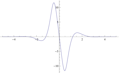
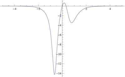
Figure 6: Plots of the density of the first integral of motion as a function of $x$ evaluated on the stationary quadruplet soliton (3.29) for $\alpha=\beta=\gamma=\omega=1$, $\delta=0$ (left panel) and for the stationary doublet soliton (3.31) for $\kappa=\sigma_{0}=1$, $\phi=0$ (right panel).

Similarly, for the second matrix $\mathcal{L}_{1}$ one needs to extract the diagonal part of (6.2). The result reads

$$\big{(}U^{f}_{0}p_{1}\big{)}^{d}=\mathcal{L}_{1}.$$ (6.8)

After substituting the expression (6.7) for $p_{1}$ into (6.8) one obtains

$$\mathcal{L}_{1}=\frac{1}{8}\left[|uu^{*}_{x}+vv^{*}_{x}|^{2}+4|uv_{x}-vu_{x}|^{2}\right]\left(\begin{array}[]{ccc}1&0&0\\ 0&0&0\\ 0&0&-1\end{array}\right).$$

Hence the second integral density is $\mathcal{I}_{1}=|uu^{*}_{x}+vv^{*}_{x}|^{2}+4|uv_{x}-vu_{x}|^{2}$.

In general, one is able to calculate the-$k$ integral of motion through the formula

$$\mathcal{L}_{k}=\big{(}U^{f}_{0}p_{k}\big{)}^{d}.$$

The matrix $p_{k}$ in its turn is obtained from the following recursive formula

$$p_{k}=-\mathop{\rm ad}\nolimits^{-1}_{J}\left(ip_{k-1,x}+(U_{0}p_{k-1})^{f}-\sum^{k-1}_{m=0}p_{k-1-m}\mathcal{L}_{m}\right).$$

6.2 The hierarchy of NLEE – Lax pair approach

Our goal here is to describe the hierarchy of integrable NLEEs associated to the Lax operator (2.3) in terms of the operators $\Lambda_{1}$ and $\Lambda_{2}$. In order to achieve it we shall analyze the recurrence relations obtained form the zero curvature representation $[L,A]=0$.

An arbitrary member of the integrable hierarchy under consideration has a Lax pair in the form

$$L(\lambda)=i\partial_{x}+\lambda L_{1}(x,t),\qquad A(\lambda)=i\partial_{t}+\sum^{N}_{k=1}\lambda^{k}A_{k}(x,t).$$

As before the operators $L$ and $A$ are subject to the action of the reductions (2.16), (2.17). Hence the coefficients of $A$ are hermitian matrices to fulfill

$$\mathbf{C}A_{2q-1}\mathbf{C}=-A_{2q-1}\!\quad\Rightarrow\quad\!A_{2q-1}\in\mathfrak{sl}^{1}(3),\qquad\mathbf{C}A_{2q}\mathbf{C}=A_{2q}\!\quad\Rightarrow\quad\!A_{2q}\in\mathfrak{sl}^{0}(3).$$

Thus the original Lax pair (2.3), (2.4) represents the simplest nontrivial flow ($N=2$) of the above general flow pair.

The compatibility condition $[L(\lambda),A(\lambda)]=0$ gives the following set of recurrence relations:

$$[L_{1},A_{N}]=0,$$ (6.9)

$$i\partial_{x}A_{N}+[L_{1},A_{N-1}]=0,$$ (6.10)

$$\cdots\cdots\cdots\cdots\cdots\cdots\cdots\cdots$$

$$i\partial_{x}A_{k}+[L_{1},A_{k-1}]=0,\qquad k=2,\ldots,N-1,$$ (6.11)

$$\cdots\cdots\cdots\cdots\cdots\cdots\cdots\cdots\cdots\cdots\cdots\cdots$$

$$\partial_{x}A_{1}-\partial_{t}L_{1}=0.$$ (6.12)

It directly follows from the first relation that the highest order term is a polynomial of $L_{1}$. Since $L_{1}\in\mathfrak{sl}^{1}(3)$ and $L_{2}\in\mathfrak{sl}^{0}(3)$ we have two options for $A_{N}$:

$${\rm a)}\quad A_{N}=f_{2p}L_{2}\quad\mbox{for}\quad N=2p,\qquad{\rm b)}\quad A_{N}=f_{2p+1}L_{1}\quad\mbox{for}\quad N=2p+1.$$

It suffices to restrict ourselves with the case when $N=2p$ since the case $N=2p+1$ is completely analogous.

As we did many times in our exposition we shall split each element $A_{k}$ into two mutually orthogonal parts $A^{\bot}_{2q-1}$ and $f_{2q-1}L_{1}$ (resp. $A^{\bot}_{2q}$ and $f_{2q}L_{2}$ in the case even indices):

$$A_{2q-1}=A^{\bot}_{2q-1}+f_{2q-1}L_{1},\qquad A_{2q}=A^{\bot}_{2q}+f_{2q}L_{2}.$$ (6.13)

Substituting the splitting of $A_{N-1}$ into (6.10) we have

$$if_{2p,x}L_{2}+if_{2p}L_{2,x}+[L_{1},A^{\bot}_{2p-1}]=0.$$

After taking the Killing form $\langle\,\cdot\,,L_{2}\rangle$ to separate the $L_{1}$-commuting part and its orthogonal complement we deduce that $f_{N}=c_{N}=\mbox{const}$ and

$$A^{\bot}_{2p-1}=-ic_{2p}\mathop{\rm ad}\nolimits^{-1}_{L_{1}}L_{2,x}.$$

Similarly, after inserting the splitting (6.13) into a generic recurrence relation (6.11) we obtain

$$if_{2q-1,x}L_{1}+if_{2q-1}L_{1,x}+i\big{(}A^{\bot}_{2q-1}\big{)}_{x}+[L_{1},A^{\bot}_{2q-2}]=0,$$

$$if_{2q,x}L_{2}+if_{2q}L_{2,x}+i\big{(}A^{\bot}_{2q}\big{)}_{x}+[L_{1},A^{\bot}_{2q-1}]=0.$$

After extracting the $L_{1}$-commuting part from the equations above one obtains the coefficient $f_{2q-1}$ (resp. $f_{2q}$)

$$f_{2q-1}=c_{2q-1}-\frac{1}{2}\partial^{-1}_{x}\langle\big{(}A^{\bot}_{2q-1}\big{)}_{x},L_{1}\rangle,\qquad f_{2q}=c_{2q}-\frac{3}{2}\partial^{-1}_{x}\langle\big{(}A^{\bot}_{2q}\big{)}_{x},L_{2}\rangle,$$

where $c_{2q-1}$ (resp. $c_{2q}$) is a constant of integration. On the other hand for $A^{\bot}_{2q-1}$ (resp. $A^{\bot}_{2q}$) we have:

$$A^{\bot}_{2q}=\Lambda_{1}\big{(}A^{\bot}_{2q+1}\big{)}-ic_{2q+1}\mathop{\rm ad}\nolimits^{-1}_{L_{1}}L_{1,x},\qquad A^{\bot}_{2q-1}=\Lambda_{2}\big{(}A^{\bot}_{2q}\big{)}-ic_{2q}\mathop{\rm ad}\nolimits^{-1}_{L_{1}}L_{2,x},$$

where the integro-differential operators $\Lambda_{2}$ and $\Lambda_{1}$ are given by (4.10) and (4.11) respectively.

The last recurrence relation (6.12) yields to

$$f_{1}=c_{1}-\frac{1}{2}\partial^{-1}_{x}\langle(A^{\bot}_{1})_{x},L_{1}\rangle,\qquad i\mathop{\rm ad}\nolimits_{L_{1}}^{-1}\partial_{t}L_{1}+\Lambda_{1}A^{\bot}_{1}-ic_{1}\mathop{\rm ad}\nolimits^{-1}_{L_{1}}{L}_{1,x}=0.$$

What remains is to substitute consequently the expressions for $A^{\bot}_{k}$, $k=1,\ldots,2p-1$ above in order to write the NLEE in terms of the operators $\Lambda_{1}$ and $\Lambda_{2}$. Here we give the results for both cases a) and b):

$${\rm a)}\quad\mathop{\rm ad}\nolimits^{-1}_{L_{1}}\partial_{t}L_{1}-\sum_{q=1}^{p}c_{2q}(\Lambda_{1}\Lambda_{2})^{q-1}\Lambda_{1}\mathop{\rm ad}\nolimits_{L_{1}}^{-1}L_{2,x}-\sum_{q=0}^{p-1}c_{2q+1}(\Lambda_{1}\Lambda_{2})^{q}\mathop{\rm ad}\nolimits_{L_{1}}^{-1}L_{1,x}=0,$$

$${\rm b)}\quad\mathop{\rm ad}\nolimits^{-1}_{L_{1}}\partial_{t}L_{1}-\sum_{q=1}^{p}c_{2q}(\Lambda_{1}\Lambda_{2})^{q-1}\Lambda_{1}\mathop{\rm ad}\nolimits_{L_{1}}^{-1}L_{2,x}-\sum_{q=0}^{p}c_{2q+1}(\Lambda_{1}\Lambda_{2})^{q}\mathop{\rm ad}\nolimits_{L_{1}}^{-1}L_{1,x}=0.$$ (6.14)

The coefficients $c_{k}$ are involved in dispersion laws of NLEEs. By analogy with (2.30) the dispersion law of a general NLEE is defined through

$$f(\lambda)=\lim_{x\to\pm\infty}g_{\pm}^{-1}\sum^{N}_{k=1}\lambda^{k}A_{k}(x,t)g_{\pm}.$$

The dispersion law governs the time evolution of scattering matrix (2.31) through the linear equation

$$i\partial_{t}T(t,\lambda)+[f(\lambda),T(t,\lambda)]=0\quad\Rightarrow\quad T(t,\lambda)=e^{if(\lambda)t}T(0,\lambda)e^{-if(\lambda)t}.$$ (6.15)

It is not hard to check that the equalities below are valid

$${\rm a)}\quad f(\lambda)=\sum_{q=0}^{p-1}c_{2q+1}\lambda^{2q+1}J+\sum_{q=1}^{p}c_{2q}\lambda^{2q}I,$$

$${\rm b)}\quad f(\lambda)=\sum_{q=0}^{p}c_{2q+1}\lambda^{2q+1}J+\sum_{q=1}^{p}c_{2q}\lambda^{2q}I.$$ (6.16)

We remind that the constant diagonal matrices $J$ and $I$ represent the diagonal forms of the asymptotic of $L_{1}$ and $L_{2}$ respectively, see (2.22), (2.23). As one can easily convince himself the initial NLEE (2.1) can be derived from the above formulae in the simplest case $N=2$ after plugging $c_{2}=-1$ and $c_{1}=0$.

6.3 The hierarchy of NLEE and generalized Fourier transforms

In the previous subsection we described the class of NLEE related to the Lax operator $L$. In particular we showed that if $L_{1}(x,t)$ is a solution to one of the NLEE (6.14) then the corresponding scattering matrix $T(\lambda,t)$ satisfies the linear evolution equation (6.15) with dispersion law $f(\lambda)$ given by (6.16).

Here we will prove a more general theorem.

Theorem 6.1.

Let the Lax operator $L$ be such that its potential satisfies the conditions C1)–C3). Then the NLEE (6.14) are equivalent to each of the following set of linear evolution equations:

$$i\frac{\partial S^{+}}{\partial t}+[f(\lambda),S^{+}(\lambda)]=0,\qquad i\frac{\partial D^{+}}{\partial t}=0,\qquad i\frac{\partial S^{-}}{\partial t}+[f(\lambda),S^{-}(\lambda)]=0,$$

$$i\frac{\partial s^{+}_{k}}{\partial t}+[f(\lambda_{k}^{+}),s^{+}_{k}]=0,\qquad i\frac{\partial\lambda_{k}^{\pm}}{\partial t}=0,\qquad i\frac{\partial s^{-}_{k}}{\partial t}+[f(\lambda_{k}^{-}),s^{-}_{k}]=0;$$ (6.17)

$$i\frac{\partial T^{-}}{\partial t}+[f(\lambda),T^{-}(\lambda)]=0,\qquad i\frac{\partial D^{-}}{\partial t}=0,\qquad i\frac{\partial T^{+}}{\partial t}+[f(\lambda),T^{+}(\lambda)]=0,$$

$$i\frac{\partial r^{-}_{k}}{\partial t}+[f(\lambda_{k}^{+}),r^{-}_{k}]=0,\qquad i\frac{\partial\lambda_{k}^{\pm}}{\partial t}=0,\qquad i\frac{\partial r^{+}_{k}}{\partial t}+[f(\lambda_{k}^{-}),r^{+}_{k}]=0.$$ (6.18)

Proof 6.2.

Let us first consider the NLEE (6.14a) and let us denote its left hand side by $N_{\rm a)}(x,t)$. Next let us expand it over the complete set of eigenfunctions $H^{\pm}_{\pm\alpha}(x,\lambda)$. If we make use of the expansion (5.11) then we need to calculate the expansion coefficients (5.12). Using the properties of the recursion operators (5.16) and (5.17) we have:

$$\gamma^{\pm}_{N_{\rm a)}}(\lambda)=\big{[}\big{[}e^{\pm}_{\mp\alpha}(y,\lambda),\mathop{\rm ad}\nolimits_{L_{1}}^{-1}N_{\rm a)}(y)\big{]}\big{]}$$

$$\phantom{\gamma^{\pm}_{N_{\rm a)}}(\lambda)}{}=\big{[}\big{[}H^{\pm}_{\mp\alpha}(y,\lambda),L_{1,t}\big{]}\big{]}-\sum_{q=1}^{p}c_{2q}\big{[}\big{[}K^{\pm}_{\mp\alpha}(y,\lambda),(\Lambda^{-,\ast})^{q-1}\Lambda_{1}^{-}\mathop{\rm ad}\nolimits_{L_{1}}^{-1}L_{2,x}\big{]}\big{]}$$

$$\phantom{\gamma^{\pm}_{N_{\rm a)}}(\lambda)=}{}-\sum_{q=0}^{p-1}c_{2q+1}\big{[}\big{[}K^{\pm}_{\mp\alpha}(y,\lambda),(\Lambda^{-,\ast})^{q}\mathop{\rm ad}\nolimits_{L_{1}}^{-1}L_{1,x}\big{]}\big{]}$$

$$\phantom{\gamma^{\pm}_{N_{\rm a)}}(\lambda)}{}=\frac{i}{\lambda}\delta_{t}\tau_{\alpha}^{\pm}(\lambda)+\sum_{q=1}^{p}c_{2q}\big{[}\big{[}\Lambda_{1}^{+}(\Lambda^{+})^{q-1}K^{\pm}_{\mp\alpha}(y,\lambda),\mathop{\rm ad}\nolimits_{L_{1}}^{-1}L_{2,x}\big{]}\big{]}$$

$$\phantom{\gamma^{\pm}_{N_{\rm a)}}(\lambda)=}{}+\sum_{q=0}^{p-1}c_{2q+1}\big{[}\big{[}(\Lambda^{+})^{q}K^{\pm}_{\mp\alpha}(y,\lambda),\mathop{\rm ad}\nolimits_{L_{1}}^{-1}L_{1,x}\big{]}\big{]}$$

$$\phantom{\gamma^{\pm}_{N_{\rm a)}}(\lambda)}{}=\frac{i}{\lambda}\delta_{t}\tau_{\alpha}^{\pm}(\lambda)+\sum_{q=1}^{p}c_{2q}\lambda^{2q-1}\big{[}\big{[}H^{\pm}_{\mp\alpha}(y,\lambda),\mathop{\rm ad}\nolimits_{L_{1}}^{-1}L_{2,x}\big{]}\big{]}$$

$$\phantom{\gamma^{\pm}_{N_{\rm a)}}(\lambda)=}{}+\sum_{q=0}^{p-1}c_{2q+1}\lambda^{2q+1}\big{[}\big{[}K^{\pm}_{\mp\alpha}(y,\lambda),\mathop{\rm ad}\nolimits_{L_{1}}^{-1}L_{1,x}\big{]}\big{]}$$

$$\phantom{\gamma^{\pm}_{N_{\rm a)}}(\lambda)}{}=\frac{1}{\lambda}\left(i\left\langle\hat{S}^{\pm}\frac{\partial S^{\pm}}{\partial t},E_{\mp\alpha}\right\rangle+\langle\hat{S}^{\pm}f(\lambda)S^{\pm}(\lambda),E_{\mp\alpha}\rangle\right)=0\quad\mbox{for all}\quad\alpha\in\Delta_{+}.$$ (6.19)

From equation (6.19) we find that

$$i\hat{S}^{\pm}\frac{\partial S^{\pm}}{\partial t}+\hat{S}^{+}f(\lambda)S^{\pm}(\lambda)=\mathcal{H}(\lambda),$$ (6.20)

where $\mathcal{H}(\lambda)\in\mathfrak{h}$. It remains to take the Killing form of (6.20) with the Cartan elements $J$ and $I$ of $\mathfrak{sl}$ to determine that $\mathcal{H}(\lambda)=f(\lambda)$. Thus we have proved that from the NLEE one gets the first of the equations in (6.17):

$$i\frac{\partial S^{\pm}}{\partial t}+[f(\lambda),S^{\pm}(\lambda)]=0.$$

Next we rewrite equation (2.35) in the form:

$$\hat{D}^{+}\hat{T}^{-}T^{+}D^{-}(\lambda)=\hat{S}^{+}S^{-}(\lambda),$$

and equate the principle upper- and lower-minors of both sides. As a result we get:

$$\frac{1}{m_{1}^{+}m_{2}^{-}}=1-s^{+}_{\alpha_{1}}s^{-}_{\alpha_{1}}-s^{+}_{\alpha_{3}}s^{-}_{\alpha_{3}}+\frac{1}{2}(s^{+}_{\alpha_{1}}s^{+}_{\alpha_{2}}s^{-}_{\alpha_{3}}-s^{-}_{\alpha_{1}}s^{-}_{\alpha_{2}}s^{+}_{\alpha_{3}})+\frac{1}{4}s^{+}_{\alpha_{1}}s^{-}_{\alpha_{1}}s^{+}_{\alpha_{2}}s^{-}_{\alpha_{2}},$$

$$\frac{1}{m_{2}^{+}m_{1}^{-}}=1-s^{+}_{\alpha_{2}}s^{-}_{\alpha_{2}}-s^{+}_{\alpha_{3}}s^{-}_{\alpha_{3}}-\frac{1}{2}(s^{+}_{\alpha_{1}}s^{+}_{\alpha_{2}}s^{-}_{\alpha_{3}}-s^{-}_{\alpha_{1}}s^{-}_{\alpha_{2}}s^{+}_{\alpha_{3}})+\frac{1}{4}s^{+}_{\alpha_{1}}s^{-}_{\alpha_{1}}s^{+}_{\alpha_{2}}s^{-}_{\alpha_{2}}$$ (6.21)

and

$$\frac{1}{m_{2}^{+}m_{1}^{-}}=1-r^{+}_{\alpha_{2}}r^{-}_{\alpha_{2}}-r^{+}_{\alpha_{3}}r^{-}_{\alpha_{3}}-\frac{1}{2}(r^{+}_{\alpha_{1}}r^{+}_{\alpha_{2}}r^{-}_{\alpha_{3}}-r^{-}_{\alpha_{1}}r^{-}_{\alpha_{2}}r^{+}_{\alpha_{3}})+\frac{1}{4}r^{+}_{\alpha_{1}}r^{-}_{\alpha_{1}}r^{+}_{\alpha_{2}}r^{-}_{\alpha_{2}},$$

$$\frac{1}{m_{1}^{+}m_{2}^{-}}=1-r^{+}_{\alpha_{1}}r^{-}_{\alpha_{1}}-r^{+}_{\alpha_{3}}r^{-}_{\alpha_{3}}+\frac{1}{2}(r^{+}_{\alpha_{1}}r^{+}_{\alpha_{2}}r^{-}_{\alpha_{3}}-r^{-}_{\alpha_{1}}r^{-}_{\alpha_{2}}r^{+}_{\alpha_{3}})+\frac{1}{4}r^{+}_{\alpha_{1}}r^{-}_{\alpha_{1}}r^{+}_{\alpha_{2}}r^{-}_{\alpha_{2}}$$ (6.22)

for $\lambda\in{\mathbb{R}}$. We remind that the scalar functions $m_{1}^{+}(\lambda)$ and $m_{2}^{+}(\lambda)$ (resp. $m_{1}^{-}(\lambda)$ and $m_{2}^{-}(\lambda)$) are analytic functions for $\lambda\in{\mathbb{C}}_{+}$ (resp. $\lambda\in{\mathbb{C}}_{-}$). Then the relations (6.21) can be viewed as a RHP which can be solved by the Plemelj–Sokhotsky formulae. Thus equations (6.21) allow us to recover $m_{1}^{\pm}(\lambda)$ and $m_{2}^{\pm}(\lambda)$, and effectively $D^{\pm}(\lambda)$ in their whole regions of analyticity from $S^{\pm}(\lambda)$. Likewise, equations (6.22) allow us to recover $D^{\pm}(\lambda)$ from $T^{\pm}(\lambda)$.

From equations (6.21) there also follows that

$$\frac{dm_{k}^{\pm}}{dt}=0,\qquad k=1,2,\qquad\mbox{i.e.}\qquad\frac{dD^{\pm}}{dt}=0.$$

We can also reconstruct $T^{\pm}(\lambda)$ as the Gauss factors of $D^{+}\hat{S}^{+}S^{-}\hat{D}^{-}(\lambda)$ and check that

$$i\partial_{t}T^{\pm}(t,\lambda)+[f(\lambda),T^{\pm}(t,\lambda)]=0.$$

Thus we have proved the statement of the theorem for the scattering data on the continuous spectrum of $L$. Similar procedure allows us to recover the equations for the data on the discrete spectrum of $L$.

In order to complete the proof of the equivalence between the NLEE (6.14) and (6.17) it remains to apply Corollary 5.2.

The equivalence of the NLEE (6.14) and (6.18) is proved along the same lines analyzing the expansion coefficients $\theta^{\pm}_{N_{\rm a)}}(\lambda)$.

As an immediate consequence of the theorem we obtain:

Corollary 6.3.

Each of the minimal sets of scattering data $\mathcal{S}_{k}$, $k=1,2$:

$$\mathcal{S}_{1}=\big{\{}s_{\alpha}^{+}(\lambda),s_{\alpha}^{-}(\lambda),\ \lambda\in{\mathbb{R}},\ s_{\alpha;k}^{+},s_{\alpha;k}^{-},\lambda_{k}^{\pm},\ \alpha\in\Delta_{+},\ k=1,\dots,2N_{1}+N_{2}\big{\}},$$

$$\mathcal{S}_{2}=\big{\{}r_{\alpha}^{+}(\lambda),r_{\alpha}^{-}(\lambda),\ \lambda\in{\mathbb{R}},\ r_{\alpha;k}^{+},r_{\alpha;k}^{-},\lambda_{k}^{\pm},\ \alpha\in\Delta_{+},\ k=1,\dots,2N_{1}+N_{2}\big{\}},$$

determines uniquely both the scattering matrix $T(\lambda)$ and the potential $L_{1}(x)$ of the Lax operator $L$.

Proof 6.4.

The fact that each of the sets $\mathcal{S}_{k}$ determine the scattering matrix $T(\lambda)$ follows easily from the Theorem. Indeed, we showed how, starting from $\mathcal{S}_{k}$ one can construct each of the Gauss factors of $T(\lambda)$; so it remains just to take the corresponding products.

In order to reconstruct the corresponding potential we have to solve the RHP with canonical normalization for $\lambda=0$. Considering the Taylor expansion of $\chi^{\pm}(x,\lambda)$:

$$\chi^{\pm}(x,\lambda)=\leavevmode\hbox{\small 1\kern-3.3pt\normalsize 1}+\sum_{n=1}^{\infty}\lambda^{s}\chi^{\pm}_{(s)}(x),$$

we get

$$L_{1}(x)=-i\frac{d\chi^{\pm}_{(1)}(x)}{dx}.$$ ∎

6.4 Hierarchy of Hamiltonian formulations

Our analysis here is again based on the Wronskian relations, extending the ones in Section 4. We first use slightly modified equation (4.18):

$$\left\langle\hat{\chi}^{\pm}\delta\chi^{\pm}(x,\lambda),J\right\rangle\big{|}_{-\infty}^{\infty}=i\lambda\int_{-\infty}^{\infty}dx\,\left\langle\delta L_{1},h_{J}^{\pm}(x,\lambda)\right\rangle,$$

$$\left\langle\hat{\chi}^{\pm}\delta\chi^{\pm}(x,\lambda),I\right\rangle\big{|}_{-\infty}^{\infty}=i\lambda\int_{-\infty}^{\infty}dx\,\left\langle\delta L_{1},h_{I}^{\pm}(x,\lambda)\right\rangle,$$

where

$$h_{J}^{\pm}(x,\lambda)=\chi^{\pm}(x,\lambda)J\hat{\chi}^{\pm}(x,\lambda),\qquad h_{I}^{\pm}(x,\lambda)=\chi^{\pm}(x,\lambda)I\hat{\chi}^{\pm}(x,\lambda).$$

A third class of Wronskian relations connects the variation of the derivative $\dot{\chi}(x,\lambda)\equiv\partial_{\lambda}\chi(x,\lambda)$ with $L_{1}$, i.e.

$$\left\langle\hat{\chi}^{\pm}\dot{\chi}^{\pm}(x,\lambda),J\right\rangle\big{|}_{-\infty}^{\infty}=-\int_{-\infty}^{\infty}dx\,\left\langle L_{1},h_{J}^{\pm}(x,\lambda)\right\rangle,$$

$$\left\langle\hat{\chi}^{\pm}\dot{\chi}^{\pm}(x,\lambda),I\right\rangle\big{|}_{-\infty}^{\infty}=-\int_{-\infty}^{\infty}dx\,\left\langle L_{1},h_{I}^{\pm}(x,\lambda)\right\rangle.$$

Thus we derive the interrelations between the generating functionals of integrals of motion and the corresponding potential:

$$\langle\hat{D}^{\pm}\delta D^{\pm},J\rangle\equiv\pm\delta\ln(m_{1}^{\pm}m_{2}^{\pm})=-i\lambda\big{[}\big{[}\mathop{\rm ad}\nolimits_{L_{1}}^{-1}\delta L_{1},h_{J}^{\pm}(x,\lambda)\big{]}\big{]},$$

$$\langle\hat{D}^{\pm}\delta D^{\pm},I\rangle\equiv\delta\ln\frac{m_{1}^{\pm}}{m_{2}^{\pm}}=-i\lambda\big{[}\big{[}\mathop{\rm ad}\nolimits_{L_{1}}^{-1}\delta L_{1},h_{I}^{\pm}(x,\lambda)\big{]}\big{]}.$$

Note that the second reduction in equation (2.33) applied to $h_{J}^{\pm}(x,\lambda)$ and $h_{I}^{\pm}(x,\lambda)$ gives

$$\mathbf{C}h_{J}^{\pm}(x,-\lambda)\mathbf{C}=-h_{J}^{\pm}(x,\lambda),\qquad\mathbf{C}h_{I}^{\pm}(x,-\lambda)\mathbf{C}=h_{I}^{\pm}(x,\lambda),$$

which means that

$$\pm\ln(m_{1}^{\pm}m_{2}^{\pm})=\sum_{s=1}^{\infty}\lambda^{-2s-1}C_{J;2s+1},\qquad\ln\frac{m_{1}^{\pm}}{m_{2}^{\pm}}=\sum_{s=1}^{\infty}\lambda^{-2s}C_{I;2s},$$

where $C_{J;2s+1}$ and $C_{I;2s}$ are integrals of motion.

Let us note that neither $h_{J}^{\pm}(x,\lambda)$ nor $h_{I}^{\pm}(x,\lambda)$ are eigenfunctions of the recursion operators. Indeed, if we separate the ‘orthogonal’ and ‘parallel’ to $L_{1}$ and $L_{2}$ parts and split them into:

$$h_{J}^{\pm,\perp}(x,\lambda)=H_{J}^{\pm}(x,\lambda)+K_{J}^{\pm}(x,\lambda),\qquad h_{I}^{\pm,\perp}(x,\lambda)=H_{I}^{\pm}(x,\lambda)+K_{I}^{\pm}(x,\lambda),$$

we get:

$$\Lambda_{1}^{\pm}K_{J}^{\pm}(x,\lambda)=\lambda H_{J}^{\pm}(x,\lambda)+i\mathop{\rm ad}\nolimits_{L_{1}}^{-1}L_{1,x},\qquad \Lambda_{2}^{\pm}H_{J}^{\pm}(x,\lambda)=\lambda K_{J}^{\pm}(x,\lambda),$$

$$\Lambda_{1}^{\pm}K_{I}^{\pm}(x,\lambda)=\lambda H_{I}^{\pm}(x,\lambda),\qquad \Lambda_{2}^{\pm}H_{I}^{\pm}(x,\lambda)=\lambda K_{I}^{\pm}(x,\lambda)+i\mathop{\rm ad}\nolimits_{L_{1}}^{-1}L_{2,x}.$$

Therefore

$$(\Lambda_{2}^{\pm}\Lambda_{1}^{\pm}-\lambda^{2})K_{J}^{\pm}(x,\lambda)=i\Lambda_{2}^{\pm}\mathop{\rm ad}\nolimits_{L_{1}}^{-1}L_{1,x},\qquad (\Lambda_{1}^{\pm}\Lambda_{2}^{\pm}-\lambda^{2})H_{J}^{\pm}(x,\lambda)=i\lambda\mathop{\rm ad}\nolimits_{L_{1}}^{-1}L_{1,x},$$

$$(\Lambda_{2}^{\pm}\Lambda_{1}^{\pm}-\lambda^{2})K_{I}^{\pm}(x,\lambda)=i\lambda\mathop{\rm ad}\nolimits_{L_{1}}^{-1}L_{2,x},\qquad (\Lambda_{1}^{\pm}\Lambda_{2}^{\pm}-\lambda^{2})H_{I}^{\pm}(x,\lambda)=i\Lambda_{1}^{\pm}\mathop{\rm ad}\nolimits_{L_{1}}^{-1}L_{1,x}$$

and

$$\pm\delta\ln(m_{1}^{\pm}m_{2}^{\pm})=\sum_{s=0}^{\infty}\lambda^{-2s-1}\delta C_{J,2s+1}=\lambda\big{[}\big{[}\mathop{\rm ad}\nolimits_{L_{1}}^{-1}\delta L_{1},(\Lambda_{2}\Lambda_{1}-\lambda^{2})^{-1}\Lambda_{2}\mathop{\rm ad}\nolimits_{L_{1}}^{-1}L_{1,x}\big{]}\big{]},$$

$$\delta\ln\frac{m_{1}^{\pm}}{m_{2}^{\pm}}=\sum_{s=0}^{\infty}\lambda^{-2s}\delta C_{I,2s}=\lambda^{2}\big{[}\big{[}\mathop{\rm ad}\nolimits_{L_{1}}^{-1}\delta L_{1},(\Lambda_{2}\Lambda_{1}-\lambda^{2})^{-1}\mathop{\rm ad}\nolimits_{L_{1}}^{-1}L_{2,x}\big{]}\big{]},$$

or in other words

$$\delta C_{J,2s+1}=-\big{[}\big{[}\mathop{\rm ad}\nolimits_{L_{1}}^{-1}\delta L_{1},(\Lambda_{2}\Lambda_{1})^{s}\Lambda_{2}\mathop{\rm ad}\nolimits_{L_{1}}^{-1}\delta L_{1,x}\big{]}\big{]},$$

$$\delta C_{I,2s}=-\big{[}\big{[}\mathop{\rm ad}\nolimits_{L_{1}}^{-1}\delta L_{1},(\Lambda_{2}\Lambda_{1})^{s}\mathop{\rm ad}\nolimits_{L_{1}}^{-1}\delta L_{2,x}\big{]}\big{]}.$$ (6.23)

We can rewrite equations (6.23) in the form:

$$\frac{\delta C_{J,2s+1}}{\delta L_{1}(x)}=(\Lambda_{2}\Lambda_{1})^{s}\Lambda_{2}\mathop{\rm ad}\nolimits_{L_{1}}^{-1}L_{1,x},\qquad\frac{\delta C_{I,2s}}{\delta L_{1}(x)}=(\Lambda_{2}\Lambda_{1})^{s}\mathop{\rm ad}\nolimits_{L_{1}}^{-1}L_{1,x}.$$

Thus in fact we have proved that the conserved quantities of these NLEE satisfy the well known Lenart relation

$$\frac{\delta C_{J,2s+1}}{\delta L_{1}(x)}=\Lambda_{2}\Lambda_{1}\frac{\delta C_{J,2s-1}}{\delta L_{1}(x)},\qquad\frac{\delta C_{I,2s}}{\delta L_{1}(x)}=\Lambda_{2}\Lambda_{1}\frac{\delta C_{I,2s-2}}{\delta L_{1}(x)}.$$ (6.24)

We finish by formulating the Hamiltonian properties of these NLEE. It is only natural that the Hamiltonians must be linear combinations of integrals of motion:

$$H_{\rm a)}=\sum_{q=0}^{p-1}c_{2q+1}C_{J,2q+1}+\sum_{q=0}^{p}c_{2q}C_{I,2q},\qquad H_{\rm b)}=\sum_{q=0}^{p}c_{2q+1}C_{J,2q+1}+\sum_{q=0}^{p}c_{2q}C_{I,2q}.$$

Next we introduce a symplectic structure using the symplectic form:

$$\Omega_{1}=\big{[}\big{[}\mathop{\rm ad}\nolimits_{L_{1}}^{-1}\delta L_{1}\mathop{\wedge}\limits_{{}^{\prime}}\Lambda_{2}\mathop{\rm ad}\nolimits_{L_{1}}^{-1}\delta L_{1}\big{]}\big{]}.$$

Using (6.24) we find that the equation of motion (6.14) can be written down as

$$\Omega_{1}^{\vee}\equiv\big{[}\big{[}\mathop{\rm ad}\nolimits_{L_{1}}^{-1}\delta L_{1}\cdot\Lambda_{2}\mathop{\rm ad}\nolimits_{L_{1}}^{-1}L_{1,t}\big{]}\big{]}=\delta H,$$ (6.25)

with $H=H_{\rm a)}$ or $H=H_{\rm b)}$ respectively.

In particular, choosing $H=C_{I,2}$ we find that equation (6.25) becomes

$$\Omega_{1}\big{(}\,\cdot\,,\mathop{\rm ad}\nolimits_{L_{1}}^{-1}\delta L_{1,t}\big{)}=\delta C_{I,2}$$

and coincides with the reduced HF equation (2.1) we started with.

Along with $\Omega_{1}$ we can also introduce the following hierarchy of symplectic forms:

$$\Omega_{2k-1}=\big{[}\big{[}\mathop{\rm ad}\nolimits_{L_{1}}^{-1}\delta L_{1}\mathop{\wedge}\limits_{{}^{\prime}}(\Lambda_{2}\Lambda_{1})^{k-1}\Lambda_{2}\mathop{\rm ad}\nolimits_{L_{1}}^{-1}\delta L_{1}\big{]}\big{]}.$$ (6.26)

Then we can write the equation of motion (6.14) in Hamiltonian form using each one of the above 2-forms as follows:

$$\Omega_{2k-1}^{\vee}\equiv\big{[}\big{[}\mathop{\rm ad}\nolimits_{L_{1}}^{-1}\delta L_{1}(\Lambda_{2}\Lambda_{1})^{k-1}\Lambda_{2}\mathop{\rm ad}\nolimits_{L_{1}}^{-1}L_{1,t}\big{]}\big{]}=\delta H_{2k}$$

with $H=H_{2k;{\rm a)}}$ or $H=H_{2k;{\rm b)}}$ respectively, where

$$H_{2k;{\rm a)}}=\sum_{q=0}^{p-1}c_{2q+2k+1}C_{J,2q+1}+\sum_{q=0}^{p}c_{2q}C_{I,2q+2k},$$

$$H_{2k;{\rm b)}}=\sum_{q=0}^{p}c_{2q+1}C_{J,2q+2k+1}+\sum_{q=0}^{p}c_{2q}C_{I,2q+2k}.$$

Using the expansions of $\mathop{\rm ad}\nolimits_{L_{1}}^{-1}\delta L_{1}$ over the ‘squared solutions’

$$\Omega_{2k-1}=\big{[}\big{[}\mathop{\rm ad}\nolimits_{L_{1}}^{-1}\delta L_{1}\mathop{\wedge}\limits_{{}^{\prime}}(\Lambda_{2}\Lambda_{1})^{k-1}\Lambda_{2}\mathop{\rm ad}\nolimits_{L_{1}}^{-1}\delta L_{1}\big{]}\big{]}=\frac{1}{2\pi}\int_{-\infty}^{\infty}d\lambda\lambda^{2k-1}(\Omega_{0}^{+}(\lambda)-\Omega_{0}^{-}(\lambda))$$

$$\phantom{\Omega_{2k-1}=}{}+\sum_{k=1}^{2N_{1}+N_{2}}\left(\mathop{\rm Res}\limits_{\lambda=\lambda_{k}^{+}}\lambda^{2k-1}\Omega_{0}^{+}(\lambda)+\mathop{\rm Res}\limits_{\lambda=\lambda_{k}^{-}}\lambda^{2k}\Omega_{0}^{-}(\lambda)\right),$$

where

$$\Omega_{0}^{+}(\lambda)=\sum_{\alpha\in\Delta_{+}}\delta^{\prime}\rho_{\alpha}^{\pm}(\lambda)\wedge\delta^{\prime}\tau_{\alpha}^{\pm}(\lambda).$$

Thus we conclude that the family of symplectic forms (6.26) are dynamically compatible.

7 Discussion and conclusions

A system of coupled equations, which generalize Heisenberg ferromagnet equations has been studied. The system is associated with a polynomial bundle Lax operator $L$ related to the symmetric space $SU(3)/S(U(1)\times U(2))$.

The spectral properties of the operator $L$ in the case of the simplest constant boundary condition (2.2) have been described. The continuous spectrum of $L$ fills up the real axis in the complex $\lambda$-plane and divides it into two regions: the upper half plane ${\mathbb{C}}_{+}$ and the lower half plane ${\mathbb{C}}_{-}$. Each region is an analyticity domain of a fundamental analytic solution to the auxiliary linear problem.

By using the dressing method [41, 50, 51, 52] we have constructed 1-soliton solutions of the (${\mathbb{Z}}_{2}$-HF) models. Due to the additional symmetries the Lax operator $L$ may possess two types of discrete eigenvalues: generic ones and purely imaginary ones. Therefore we will have two types of soliton solutions – quadruplet and doublet solitons respectively. We outlined the purely algebraic construction for deriving the $N$-soliton solutions for both types of solitons.

Using the Wronskian relations one is able to construct ‘squared solutions’ and an integro-differential operator called recursion operator whose eigenfunctions they are. There exists another viewpoint on recursion operator – they generate hierarchy of symmetries of NLEEs. Thus one can derive the recursion operator of a NLEE from purely symmetry considerations.

Using the interpretation of the ISM as a generalized Fourier transform and the expansions over the ‘squared solutions’ we studied the fundamental properties of the class of NLEE admitting a Lax operator of the form (2.3), including the description of the whole class of NLEE, the infinite set of integrals of motion and the Hamiltonian formulation of the corresponding hierarchy.

The results of the present article can be extended in several directions. Firstly, one can develop the theory in the case of a rational bundle $L$:

$$L=i\partial_{x}+\lambda L_{1}+\frac{1}{\lambda}L_{-1}.$$

The simplest NLEEs related to Lax pair of this type take the form

$$iu_{t}=u_{xx}-(u(u^{*}u_{x}+v^{*}v_{x}))_{x}+8vv^{*}u,$$

$$iv_{t}=v_{xx}-(v(u^{*}u_{x}+v^{*}v_{x}))_{x}-8uu^{*}v,$$ (7.1)

where $u$ and $v$ are functions of $x$ and $t$ subject to the same condition as in the polynomial case, i.e. $|u|^{2}+|v|^{2}=1$. The system (7.1) can also be seen as an anisotropic deformation of (2.1) with $k=1$, $N=3$ and is a special case of the models proposed in [24].

That modification is required when one imposes an additional ${\mathbb{Z}}_{2}$ reduction of the form $\lambda\to 1/\lambda$, see [19]. This case is more complicated and much richer than the one we have studied. It requires the construction of automorphic Lie algebras and studying their properties following the ideas of [31, 30, 47].

The second direction of generalization concerns considering Lax operator $L$ related to a generic symmetric space of the type $\mathbf{A.III}\cong SU(n+k)/S(U(n)\times U(k))$ or, more generally, related to other types of symmetric spaces. This will allow one to treat various multi-component generalizations of our NLEEs. Geometric properties of similar models related to other symmetric spaces are studied in [48].

Appendix A Parametrization of Gauss factors

Here we will list useful formulae allowing one, given the scattering matrix $T(\lambda)$ to evaluate its Gauss factors $S^{\pm}(\lambda)$, $T^{\pm}(\lambda)$ or rather $s^{\pm}(\lambda)$, $r^{\pm}(\lambda)$

$$S^{\pm}(\lambda)=\exp s^{\pm}(\lambda),\qquad T^{\pm}(\lambda)=\exp r^{\pm}(\lambda),$$

$$s^{+}(\lambda)=\left(\begin{array}[]{ccc}0&s^{+}_{\alpha_{1}}&s^{+}_{\alpha_{3}}\\ 0&0&s^{+}_{\alpha_{2}}\\ 0&0&0\end{array}\right),\qquad r^{+}(\lambda)=\left(\begin{array}[]{ccc}0&r^{+}_{\alpha_{1}}&r^{+}_{\alpha_{3}}\\ 0&0&r^{+}_{\alpha_{2}}\\ 0&0&0\end{array}\right),$$

$$s^{-}(\lambda)=\left(\begin{array}[]{ccc}0&0&0\\ s^{-}_{\alpha_{1}}&0&0\\ s^{-}_{\alpha_{3}}&s^{-}_{\alpha_{2}}&0\end{array}\right),\qquad r^{-}(\lambda)=\left(\begin{array}[]{ccc}0&0&0\\ r^{-}_{\alpha_{1}}&0&\\ r^{-}_{\alpha_{3}}&r^{-}_{\alpha_{2}}&0\end{array}\right),$$

$$D^{+}(\lambda)=\mathop{\rm diag}\nolimits(m_{1}^{+},m_{2}^{+}/m_{1}^{+},1/m_{2}^{+}),\qquad D^{-}(\lambda)=\mathop{\rm diag}\nolimits(1/m_{2}^{-},m_{2}^{-}/m_{1}^{-},m_{1}^{-}).$$

Next we insert these formulae in the left hand sides of the Wronskian relations (4.21), (4.22) and (4.23). Skipping the details we find

$$s^{+}_{\alpha_{1}}=-\frac{T_{12}}{m_{1}^{+}},\qquad s^{+}_{\alpha_{2}}=-\frac{T_{13}T_{21}-T_{23}T_{11}}{m_{2}^{+}},\qquad s^{+}_{\alpha_{3}}=\frac{T_{12}T_{23}-T_{22}T_{13}}{2m_{2}^{+}}-\frac{T_{13}}{2m_{1}^{+}},$$

$$r^{-}_{\alpha_{1}}=\frac{T_{21}}{m_{1}^{+}},\qquad r^{-}_{\alpha_{2}}=\frac{T_{11}T_{32}-T_{12}T_{31}}{m_{2}^{+}},\qquad r^{-}_{\alpha_{3}}=-\frac{T_{21}T_{32}-T_{22}T_{31}}{2m_{2}^{+}}+\frac{T_{31}}{2m_{1}^{+}},$$

$$s^{-}_{\alpha_{2}}=-\frac{T_{32}}{m_{1}^{-}},\qquad s^{-}_{\alpha_{1}}=\frac{T_{23}T_{31}-T_{21}T_{33}}{m_{2}^{-}},\qquad s^{-}_{\alpha_{3}}=\frac{T_{33}T_{21}-T_{22}T_{31}}{2m_{2}^{-}}-\frac{T_{31}}{2m_{1}^{-}},$$

$$r^{+}_{\alpha_{2}}=\frac{T_{23}}{m_{1}^{-}},\qquad r^{+}_{\alpha_{1}}=-\frac{T_{12}T_{33}-T_{13}T_{32}}{m_{2}^{-}},\qquad r^{+}_{\alpha_{3}}=\frac{T_{13}T_{22}-T_{23}T_{11}}{2m_{2}^{-}}+\frac{T_{13}}{2m_{1}^{-}};$$

$$\langle\hat{S}^{+}JS^{+}(\lambda),E_{\alpha}\rangle=(\alpha,J)s^{+}_{\alpha}(\lambda),$$

$$\langle\hat{S}^{+}IS^{+}(\lambda),E_{\alpha}\rangle=(\alpha,I)s^{+}_{\alpha}(\lambda)\quad\mbox{for}\quad\alpha=e_{1}-e_{2},e_{2}-e_{3},$$

$$\langle\hat{S}^{+}IS^{+}(\lambda),E_{e_{1}-e_{3}}\rangle=s^{+}_{12}s^{+}_{23};$$ (A.1)

$$\langle\hat{S}^{+}\delta S^{+}(\lambda),E_{\alpha}\rangle=\delta s^{+}_{\alpha}(\lambda)\quad\mbox{for}\quad\alpha=e_{1}-e_{2},e_{2}-e_{3},$$

$$\langle\hat{S}^{+}\delta S^{+}(\lambda),E_{e_{1}-e_{3}}\rangle=\delta S^{+}_{13}+\frac{1}{2}\delta(s^{+}_{12}s^{+}_{23}).$$

Thus we are able to express all expansions coefficients in terms of $s^{\pm}_{\alpha}$. The results are:

$$\tau_{\alpha}^{(1),\pm}(\lambda)\equiv\langle\hat{S}^{\pm}JS^{\pm}(\lambda),E_{\mp\alpha}\rangle=\pm(\alpha,J)s^{\pm}_{\alpha}(\lambda),$$

$$\tau_{\alpha}^{(2),\pm}(\lambda)\equiv\langle\hat{S}^{\pm}IS^{\pm}(\lambda),E_{\mp\alpha}\rangle=\left\{\left(\pm(\alpha,J)s^{\pm}_{\alpha}(\lambda)\ \mbox{for}\ \alpha\in\delta_{1}^{+}\right)\right\}\pm(\alpha,J_{2})s^{\pm}_{\alpha}(\lambda).$$

Table 1: The expansion coefficients of $\mathop{\rm ad}\nolimits_{L_{1}}^{-1}L_{j,x}$, $\mathop{\rm ad}\nolimits_{L_{1}}^{-1}\delta L_{1}$ and $\mathop{\rm ad}\nolimits_{L_{1}}^{-1}L_{1,t}$.

Roots	$\alpha_{1}=e_{1}-e_{2}$	$\alpha_{1}=e_{1}-e_{2}$	$\alpha_{1}=e_{1}-e_{2}$ 1pt 1pt
$(\alpha,J)$	1	1	2 1pt
$(\alpha,I)$	1	$-1$	0 1pt
$\tau_{\alpha}^{(1),+}(\lambda)$ 4pt	$s^{+}_{\alpha_{1}}(\lambda)$	$s^{+}_{\alpha_{2}}(\lambda)$	$2s^{+}_{\alpha_{3}}(\lambda)$
$\tau_{\alpha}^{(1),-}(\lambda)$ 2pt	$-s^{-}_{\alpha_{1}}(\lambda)$	$-s^{-}_{\alpha_{2}}(\lambda)$	$-2s^{-}_{\alpha_{3}}(\lambda)$
$\tau_{\alpha}^{(2),+}(\lambda)$4pt	$s^{+}_{\alpha_{1}}(\lambda)$	$-s^{+}_{\alpha_{2}}(\lambda)$	$s^{+}_{\alpha_{1}}s^{+}_{\alpha_{2}}(\lambda)$
$\tau_{\alpha}^{(2),-}(\lambda)$2pt	$-s^{-}_{\alpha_{1}}(\lambda)$	$s^{-}_{\alpha_{2}}(\lambda)$	$s^{-}_{\alpha_{1}}s^{-}_{\alpha_{2}}(\lambda)$
$\rho_{\alpha}^{(1),+}(\lambda)$	$-\frac{(m_{1}^{+})^{2}}{m_{2}^{+}}r^{+}_{\alpha_{1}}(\lambda)$6pt3pt	$-\frac{(m_{2}^{+})^{2}}{m_{1}^{+}}r^{+}_{\alpha_{2}}(\lambda)$	$-2m_{1}^{+}m_{2}^{+}r^{+}_{\alpha_{3}}(\lambda)$
$\rho_{\alpha}^{(1),-}(\lambda)$	$\frac{(m_{2}^{-})^{2}}{m_{1}^{-}}r^{-}_{\alpha_{1}}(\lambda)$ 5pt	$\frac{(m_{1}^{-})^{2}}{m_{2}^{-}}r^{-}_{\alpha_{2}}(\lambda)$	$2m_{1}^{-}m_{2}^{-}r^{-}_{\alpha_{3}}(\lambda)$
$\rho_{\alpha}^{(2),+}(\lambda)$	$-\frac{(m_{1}^{+})^{2}}{m_{2}^{+}}r^{+}_{\alpha_{1}}(\lambda)$6pt3pt	$-\frac{(m_{2}^{+})^{2}}{m_{1}^{+}}r^{+}_{\alpha_{2}}(\lambda)$	$m_{1}^{+}m_{2}^{+}r^{+}_{\alpha_{1}}s^{+}_{\alpha_{2}}(\lambda)$
$\rho_{\alpha}^{(2),-}(\lambda)$	$\frac{(m_{2}^{-})^{2}}{m_{1}^{-}}r^{-}_{\alpha_{1}}(\lambda)$5pt	$-\frac{(m_{1}^{-})^{2}}{m_{2}^{-}}s^{-}_{\alpha_{2}}(\lambda)$	$m_{2}^{-}m_{1}^{-}r^{-}_{\alpha_{1}}s^{-}_{\alpha_{2}}(\lambda)$
$\delta^{\prime}\tau_{\alpha}^{+}(\lambda)$	$\delta s^{+}_{\alpha_{1}}(\lambda)$	$\delta s^{+}_{\alpha_{2}}(\lambda)$	$\delta s^{+}_{\alpha_{3}}(\lambda)+\frac{1}{2}\delta s^{+}_{\alpha_{1}}s^{+}_{\alpha_{2}}(\lambda)-\frac{1}{2}\delta s^{+}_{\alpha_{2}}s^{+}_{\alpha_{1}}(\lambda)$3pt3pt
$\delta^{\prime}\tau_{\alpha}^{-}(\lambda)$	$\delta s^{-}_{\alpha_{1}}(\lambda)$	$\delta s^{-}_{\alpha_{2}}(\lambda)$	$\delta s^{-}_{\alpha_{3}}(\lambda)-\frac{1}{2}\delta s^{-}_{\alpha_{1}}s^{+}_{\alpha_{2}}(\lambda)+\frac{1}{2}\delta s^{-}_{\alpha_{2}}s^{-}_{\alpha_{1}}(\lambda)$2pt
$\delta^{\prime}_{t}\tau_{\alpha}^{+}(\lambda)$	$\frac{d}{dt}s^{+}_{\alpha_{1}}(\lambda)$	$\frac{d}{dt}s^{+}_{\alpha_{2}}(\lambda)$	$\frac{d}{dt}s^{+}_{\alpha_{3}}(\lambda)+\frac{1}{2}s^{+}_{\alpha_{2}}(\lambda)\frac{d}{dt}s^{+}_{\alpha_{1}}-\frac{1}{2}s^{+}_{\alpha_{1}}(\lambda)\frac{d}{dt}s^{+}_{\alpha_{2}}$3pt3pt
$\delta^{\prime}_{t}\tau_{\alpha}^{-}(\lambda)$	$\frac{d}{dt}s^{-}_{\alpha_{1}}(\lambda)$	$\frac{d}{dt}s^{-}_{\alpha_{2}}(\lambda)$	$\frac{d}{dt}s^{-}_{\alpha_{3}}(\lambda)-\frac{1}{2}s^{+}_{\alpha_{2}}(\lambda)\frac{d}{dt}s^{-}_{\alpha_{1}}+\frac{1}{2}s^{-}_{\alpha_{1}}(\lambda)\frac{d}{dt}s^{-}_{\alpha_{2}}$2pt

Note that varying $L_{1}$ may lead to varying the positions of the discrete eigenvalues. In order to evaluate the corresponding expansion coefficients, now we make use of the Wronskian relations (4.23). We use also the condition C2 and the explicit formulae that allow one to express all the Gauss factors $S^{\pm}(\lambda)$, $T^{\pm}(\lambda)$ and $D^{\pm}(\lambda)$ as rational expressions of the matrix elements of $T(\lambda)$. Condition C2 ensures that the Gauss factors have at most first order poles in the vicinity of $\lambda_{k}^{\pm}$. Therefore the variations of $S^{\pm}(\lambda)$ and $T^{\pm}(\lambda)$ in the vicinity of $\lambda_{k}^{\pm}$ take the form:

$$\delta s_{\alpha}^{\pm}(\lambda)\simeq(\lambda-\lambda_{k}^{\pm})^{\mp p_{\alpha}+1}\left(\frac{s_{\alpha;k}^{\pm}}{(\lambda-\lambda_{k}^{\pm})^{2}}\delta\lambda_{k}^{\pm}+\frac{\delta s_{\alpha;k}^{\pm}}{\lambda-\lambda_{k}^{\pm}}+\mathcal{O}(1)\right),$$

$$\delta r_{\alpha}^{\mp}(\lambda)\simeq(\lambda-\lambda_{k}^{\pm})^{\mp p_{\alpha}+1}\left(\frac{r_{\alpha;k}^{\mp}}{(\lambda-\lambda_{k}^{\pm})^{2}}\delta\lambda_{k}^{\pm}+\frac{\delta r_{\alpha;k}^{\mp}}{\lambda-\lambda_{k}^{\pm}}+\mathcal{O}(1)\right),$$

where $s_{\alpha;k}^{\pm}$ and $r_{\alpha;k}^{\pm}$ determine the values of the corresponding Gauss factors for $\lambda=\lambda_{k}^{\pm}$. Thus, along with the (4.23) we obtain:

$$\rho^{\pm}_{\alpha;k}\delta\lambda_{k}^{\pm}=i\lambda_{k}^{\pm}\big{[}\big{[}e^{\pm}_{\pm\alpha;k},\mathop{\rm ad}\nolimits_{L_{1}}^{-1}\delta L_{1}\big{]}\big{]},\qquad \delta^{\prime}\rho^{\pm}_{\alpha;k}=i\big{[}\big{[}e^{\pm}_{\pm\alpha;k}+\lambda_{k}^{\pm}\dot{e}^{\pm}_{\pm\alpha;k},\mathop{\rm ad}\nolimits_{L_{1}}^{-1}\delta L_{1}\big{]}\big{]},$$

$$\tau^{\pm}_{\alpha;k}\delta\lambda_{k}^{\pm}=-i\lambda_{k}^{\pm}\big{[}\big{[}e^{\pm}_{\mp\alpha;k},\mathop{\rm ad}\nolimits_{L_{1}}^{-1}\delta L_{1}\big{]}\big{]},\qquad \delta^{\prime}\tau^{\pm}_{\alpha;k}=-i\big{[}\big{[}e^{\pm}_{\mp\alpha;k}+\lambda_{k}^{\pm}\dot{e}^{\mp}_{\pm\alpha;k},\mathop{\rm ad}\nolimits_{L_{1}}^{-1}\delta L_{1}\big{]}\big{]}.$$

Remark A.1.

More precise treatment of the contribution from the discrete spectrum starts by considering the potentials for which $L_{1}(x)-L_{1,{\rm as}}$ is on finite support. Then the Jost solutions of $L$, as well as the scattering matrix $T(\lambda)$ become meromorphic functions of $\lambda$ which ensures the validity of all considerations above. The next step would be taking the limit to potentials of Schwartz-type. These considerations come out of the scope of the present paper.

When we analyze the discrete spectrum we make use of the conditions C2 and C3. Since the discrete eigenvalues are zeroes of the principal minors, and assuming that $\lambda_{k}^{+}$ (resp. $\lambda_{k}^{-}$) is a zero of, say $m_{1}^{+}(\lambda)$, then we have:

$$m_{1}^{\pm}(\lambda)=(\lambda-\lambda_{k}^{\pm})\dot{m}_{1;k}^{\pm}+\mathcal{O}\big{(}(\lambda-\lambda_{k}^{\pm})^{2}\big{)},$$

and similar expansions for $m_{2}^{\pm}(\lambda)$. Using remark 5.1 on formulae (A.1) we easily find, that $\tau_{\alpha}^{(j),\pm}(\lambda)$ have simple zeroes in the vicinity of $\lambda_{k}^{\pm}$.

We end by reminding a few useful formulae of frequently appearing expressions in the main text; they are derived in [19, 20].

Since $L_{1}$ satisfies the characteristic equation $L_{1}^{3}=L_{1}$ then $\mathop{\rm ad}\nolimits_{L_{1}}$ has eigenvalues $\pm 2$, $\pm 1$, $0$ and satisfies the characteristic equation:

$$\big{(}\mathop{\rm ad}\nolimits_{L_{1}}^{2}-4\big{)}\big{(}\mathop{\rm ad}\nolimits_{L_{1}}^{2}-1\big{)}\mathop{\rm ad}\nolimits_{L_{1}}=0$$

and therefore

$$\mathop{\rm ad}\nolimits_{L_{1}}^{-1}=\frac{1}{4}\big{(}5\mathop{\rm ad}\nolimits_{L_{1}}-\mathop{\rm ad}\nolimits_{L_{1}}^{3}\big{)}.$$

If we choose $X\in\mathfrak{sl}^{1}$ we have

$$\mathop{\rm ad}\nolimits_{L_{1}}^{-1}X=\left(\begin{array}[]{ccc}w-w^{*}&0&0\\ 0&u^{*}a-a^{*}u&u^{*}b-va^{*}\\ 0&v^{*}a-ub^{*}&v^{*}b-b^{*}v\end{array}\right)+\frac{3}{4}(w-w^{*})\left(\begin{array}[]{ccc}-1&0&0\\ 0&|u|^{2}&u^{*}v\\ 0&v^{*}u&|v|^{2}\end{array}\right),$$

where $w=ua^{*}+vb^{*}$. If in particular, $X=L_{1,x}$ we find:

$$\mathcal{L}_{1}\equiv\mathop{\rm ad}\nolimits_{L_{1}}^{-1}L_{1,x}=\left(\!\begin{array}[]{ccc}\frac{1}{2}w_{0}&0&0\\ 0&u^{*}u_{x}-u^{*}_{x}u+\frac{3}{2}w_{0}|u|^{2}&u^{*}v_{x}-vu^{*}_{x}+\frac{3}{2}w_{0}u^{*}v\\ 0&v^{*}u_{x}-uv^{*}_{x}+\frac{3}{2}w_{0}uv^{*}&v^{*}v_{x}-v^{*}_{x}v+\frac{3}{2}w_{0}|v|^{2}\end{array}\!\right),$$

where $w_{0}=uu^{*}_{x}+vv^{*}_{x}$. Similarly for $Y\in\mathfrak{sl}^{0}$ and $\mathop{\rm ad}\nolimits_{L_{1}}^{-1}Y$ we have

$$Y=\left(\!\begin{array}[]{c@{\,\,\,}c@{\,\,\,}c}-k-n&0&0\\ 0&k&m\\ 0&m^{*}&n\end{array}\!\right),\qquad\mathop{\rm ad}\nolimits_{L_{1}}^{-1}Y=\frac{1}{4}\left(\!\begin{array}[]{c@{\,\,\,}c@{\,\,\,}c}0&u\alpha_{0}+vm^{*}&v\alpha_{1}+um\\ -u^{*}\alpha_{0}-mv^{*}&0&0\\ -v^{*}\alpha_{1}-u^{*}m^{*}&0&0\end{array}\!\right),$$

$$\alpha_{0}=5k+n-3W,\qquad\alpha_{1}=k+5n-3W.$$

Choosing $Y=L_{2,x}$ we get:

$$\mathcal{L}_{2}\equiv\mathop{\rm ad}\nolimits_{L_{1}}^{-1}L_{2,x}=\left(\!\begin{array}[]{c@{\,\,\,}c@{\,\,\,}c}0&-u|u|^{2}_{x}-v(uv^{*})_{x}&-v|v|^{2}_{x}-u(v^{*}u)_{x}\\ u^{*}|u|^{2}_{x}+v^{*}(u^{*}v)_{x}&0&0\\ v|v|^{2}_{x}+u(u^{*}v)_{x}&0&0\end{array}\!\right)$$

$$\phantom{\mathcal{L}_{2}\equiv\mathop{\rm ad}\nolimits_{L_{1}}^{-1}L_{2,x}}{}=\left(\!\begin{array}[]{c@{\,\,\,}c@{\,\,\,}c}0&-u_{x}-u(uu^{*}_{x}+vv^{*}_{x})&-v_{x}-v(uu^{*}_{x}+vv^{*}_{x})\\ u^{*}_{x}+u^{*}(u^{*}u_{x}+v^{*}v_{x})&0&0\\ v^{*}_{x}+v^{*}(u^{*}u_{x}+v^{*}v_{x})&0&0\end{array}\!\right).$$

Acknowledgements

The authors have the pleasure to thank Professor Allan Fordy for numerous useful discussions. The authors acknowledge support from the Royal Society and the Bulgarian academy of sciences via joint research project “Reductions of Nonlinear Evolution Equations and analytic spectral theory”. The work of G.G.G. is supported by the Science Foundation of Ireland (SFI), under Grant no. 09/RFP/MTH2144. Finally we would like to thank one of the referees for useful suggestions.

References

- [1]
- [2] Ablowitz M.J., Kaup D.J., Newell A.C., Segur H., The inverse scattering transform – Fourier analysis for nonlinear problems, Studies in Appl. Math. 53 (1974), 249–315.
- [3] Adler V.E., Shabat A.B., Yamilov R.I., The symmetry approach to the problem of integrability, Theoret. and Math. Phys. 125 (2000), 1603–1661.
-
[4]
Athorne C., Fordy A.,
Generalised KdV and MKdV equations associated with symmetric spaces,
J. Phys. A: Math. Gen. 20 (1987), 1377–1386.
Athorne C., Fordy A., Integrable equations in dimensions associated with symmetric and homogeneous spaces, J. Math. Phys. 28 (1987), 2018–2024. - [5] Borissov A.B., Kisselev V.V., Nonlinear waves, solitons and localised structures in magnets, Vol. 1, Quasi-homogeneous magnetic solitons, Inst. Metal Physics, Ural Branch of RAS, Ekaterininburg, 2009 (in Russian).
- [6] Calogero F., Degasperis A., Nonlinear evolution equations solvable by the inverse spectral transform. I, Nuovo Cimento B 32 (1976), 201–242.
- [7] Calogero F., Degasperis A., Nonlinear evolution equations solvable by the inverse spectral transform. II, Nuovo Cimento B 39 (1976), 1–54.
- [8] Drinfel’d V.G., Sokolov V.V., Lie algebras and equations of Korteweg–de Vries type, J. Math. Sci. 30 (1985), 1975–2036.
- [9] Fordy A.P., Derivative nonlinear Schrödinger equations and Hermitian symmetric spaces, J. Phys. A: Math. Gen. 17 (1984), 1235–1245.
- [10] Fordy A.P., Kulish P.P., Nonlinear Schrödinger equations and simple Lie algebras, Comm. Math. Phys. 89 (1983), 427–443.
-
[11]
Gel’fand I.M., Dickey L.A.,
Asymptotic behaviour of the resolvent of Sturm–Liouville equations and the algebra of the Korteweg–de Vries equations,
Russ. Math. Surv. 30 (1975), no. 5, 77–1113.
Gel’fand I.M., Dickey L.A., A Lie algebra structure in a formal variational calculation, Funct. Anal. Appl. 10 (1976), no. 1, 16–22. - [12] Gerdjikov V.S., Generalised Fourier transforms for the soliton equations. Gauge-covariant formulation, Inverse Problems 2 (1986), 51–74.
- [13] Gerdjikov V.S., The generalized Zakharov–Shabat system and the soliton perturbations, Theoret. and Math. Phys. 99 (1994), 593–598.
-
[14]
Gerdjikov V.S., Grahovski G.G., Kostov N.A.,
Reductions of -wave interactions related to simple Lie algebras. I. -reductions,
J. Phys. A: Math. and Gen. 34 (2001), 9425–9461,
nlin.SI/0006001.
Gerdjikov V.S., Grahovski G.G., Ivanov R.I., Kostov N.A., -wave interactions related to simple Lie algebras. -reductions and soliton solutions, Inverse Problems 17 (2001), 999–1015, nlin.SI/0009034. - [15] Gerdjikov V.S., Grahovski G.G., Mikhailov A.V., Valchev T.I., Rational bundles and recursion operators for integrable equations on A.III-type symmetric spaces, Theoret. and Math. Phys., to appear, arXiv:1102.1942.
- [16] Gerdjikov V.S., Khristov E.Kh., On the evolution equations solvable with the inverse scattering problem. II. Hamiltonian structures and Bäcklund transformations, Bulgar. J. Phys. 7 (1980), 119–133 (in Russian).
- [17] Gerdjikov V.S., Ivanov M.I., The quadratic bundle of general form and the nonlinear evolution equations. II. Hierarchies of Hamiltonian structures, Bulgar. J. Phys. 10 (1983), 130–143 (in Russian).
- [18] Gerdjikov V.S., Kulish P.P., The generating operator for the linear system, Phys. D 3 (1981), 549–564.
- [19] Gerdjikov V.S., Mikhailov A.V., Valchev T.I., Reductions of integrable equations on A.III-type symmetric spaces, J. Phys. A: Math Theor. 43 (2010), 434015, 13 pages, arXiv:1004.4182.
- [20] Gerdjikov V.S., Mikhailov A.V., Valchev T.I., Recursion operators and reductions of integrable equations on symmetric spaces, J. Geom. Symmetry Phys. 20 (2010), 1–34.
- [21] Gerdjikov V.S., Vilasi G., Yanovski A.B., Integrable Hamiltonian hierarchies. Spectral and geometric methods, Lecture Notes in Physics, Vol. 748, Springer-Verlag, Berlin, 2008.
- [22] Golubchik I.Z., Sokolov V.V., Integrable equations on -graded Lie algebras, Theoret. and Math. Phys. 112 (1997), 1097–1103.
- [23] Golubchik I.Z., Sokolov V.V., Generalised Heisenberg equations on -graded Lie algebras, Theoret. and Math. Phys. 120 (1999), 1019–1025.
- [24] Golubchik I.Z., Sokolov V.V., Multicomponent generalization of the hierarchy of the Landau–Lifshitz equation, Theoret. and Math. Phys. 124 (2000), 909–917.
- [25] Gürses M., Karasu A., Sokolov V.V., On construction of recursion operators from Lax representation, J. Math. Phys. 40 (1999), 6473–6490, solv-int/9909003.
- [26] Helgasson S., Differential geometry, Lie groups and symmetric spaces, Pure and Applied Mathematics, Vol. 80, Academic Press, Inc., New York – London, 1978.
- [27] Ibragimov N.Kh., Shabat A.B., Infinite Lie–Bäcklund algebras, Funct. Anal. Appl. 14 (1980), 313–315.
- [28] Kaup D.J., Newell A.C., An exact solution for a derivative nonlinear Schrödinger equation, J. Math. Phys. 19 (1978), 798–801.
- [29] Lombardo S., Mikhailov A.V., Reductions of integrable equations: dihedral group, J. Phys. A: Math. Gen. 37 (2004), 7727–7742, nlin.SI/0404013.
- [30] Lombardo S., Mikhailov A.V., Reduction groups and automorphic Lie algebras, Comm. Math. Phys. 258 (2005), 179–202, math-ph/0407048.
- [31] Lombardo S., Sanders J.A., On the classification of automorphic Lie algebras, Comm. Math. Phys. 299 (2010), 793–824, arXiv:0912.1697.
- [32] Loos O., Symmetric spaces, Vol. I, General theory; Vol. II, Compact spaces and classification, W.A. Benjamin, Inc., New York – Amsterdam, 1969.
- [33] Mikhailov A.V., On the integrability of two-dimensional generalization of the Toda lattice, Lett. J. Exper. and Theor. Phys. 30 (1979), 443–448.
- [34] Mikhailov A.V., Reduction in integrable systems. The reduction group, Lett. J. Exper. and Theor. Phys. 32 (1980), 187–192.
- [35] Mikhailov A.V., The reduction problem and the inverse scattering method, Phys. D 3 (1981), 73–117.
- [36] Mikhailov A.V., The Landau–Lifschitz equation and the Riemann boundary problem on a torus, Phys. Lett. A 92 (1982), 51–55.
- [37] Mikhailov A.V., Olshanetski M.A., Perelomov A.M., Two-dimensional generalized Toda lattice, Comm. Math. Phys. 79 (1981), 473–488.
- [38] Mikhailov A.V., Sokolov V.V., Symmetries of differential equations and the problem of integrability, in Integrability, Editor A.V. Mikhailov, Lecture Notes in Physics, Vol. 767, Springer-Verlag, Berlin, 2009, 19–88.
- [39] Mikhailov A.V., Sokolov V.V., Shabat A.B., The symmetry approach to classification of integrable equations, in What is Integrability?, Editor V.E. Zakharov, Springer Ser. Nonlinear Dynam., Springer-Verlag, Berlin, 1991, 115–184.
- [40] Mikhailov A.V., Shabat A.B., Yamilov R.I., The symmetry approach to the classification of nonlinear equations. Complete lists of integrable systems, Russ. Math. Surv. 42 (1987), no. 4, 1–63.
- [41] Novikov S., Manakov S.V., Pitaevskii L.P., Zakharov V.E., Theory of solitons. The inverse scattering method, Plenum, New York, 1984.
- [42] Olver P.J., Evolution equations possessing infinitely many symmetries, J. Math. Phys. 18 (1977), 1212–1215.
- [43] Sokolov V.V., Shabat A.B., Classification of integrable evolution equations, Soviet Sci. Rev. Sect. C Math. Phys. Rev., Vol. 4, Harwood Academic Publ., Chur, 1984, 221–280.
- [44] Svinolupov S.I., Sokolov V.V., Evolution equations with nontrivial conservation laws, Funct. Anal. Appl. 16 (1982), 317–319.
- [45] Svinolupov S.I., Sokolov V.V., On conservation laws for equations with nontrivial Lie–Bäcklund algebra, in Integrable Systems, Editor A.B. Shabat, Ufa, BFAN SSSR, 1982, 53–67 (in Russian).
- [46] Takhtadjan L., Faddeev L., The Hamiltonian approach to soliton theory, Springer-Verlag, Berlin, 1986.
- [47] Wang J.P., Lenard scheme for two-dimensional periodic Volterra chain, J. Math. Phys. 50 (2009), 023506, 25 pages, arXiv:0809.3899.
- [48] Wu D., Ma H., Twisted hierarchies associated with the generalized sine-Gordon equation, arXiv:1103.6077.
-
[49]
Zakharov V.E., Manakov S.V.,
Exact theory of resonant interaction of wave packets in nonlinear media, INF preprint 74–41,
Novosibirsk, 1974, 52 pages (in Russian).
Zakharov V.E., Manakov S.V., On the theory of resonant interaction of wave packets in nonlinear media, Soviet Physics JETP 42 (1975), 842–850.
Zakharov V.E., Manakov S.V., Asymptotic behavior of nonlinear wave systems integrable by the inverse scattering method, Soviet Physics JETP 44 (1976), 106–112 (in Russian). -
[50]
Zakharov V.E., Shabat A.B.,
A scheme for integrating nonlinear equations of mathematical physics by the method of the inverse scattering transform. I,
Funct. Anal. Appl. 8 (1974), 226–235.
Zakharov V.E., Shabat A.B., Integration of nonlinear equations of mathematical physics by the method of the inverse scattering transform. II, Funct. Anal. Appl. 13 (1979), 166–174. - [51] Zakharov V.E., Mikhailov A.V., On the integrability of classical spinor models in two-dimensional space-time, Comm. Math. Phys. 74 (1980), 21–40.
- [52] Zakharov V.E., Mikhailov A.V., Relativistically invariant two-dimensional models of field theory which are integrable by means of the inverse scattering problem method, Soviet Physics JETP 47 (1978), 1017–1027.