Constraint on parameters of the Inverse Compton Scattering model for radio pulsars

Abstract

The inverse Compton scattering (ICS) model can explain various pulse profile shapes and diversity of pulse profile evolution based on the mechanism that the radio emission is generated through inverse Compton scattering between secondary relativistic particles and radio waves from polar gap avalanches. In this paper, we study the parameter space of ICS model for 15 pulsars, which share the common pulse profile evolution phenomena that the pulse profiles are narrower at higher observing frequencies. Two key parameters, the initial Lorentz factor and the energy loss factor of secondary particles are constrained using the least square fitting method, where we fit the theoretical curve of the “beam-frequency mapping” of the ICS model to the observed pulse widths at multiple frequencies. The uncertainty of the inclination and viewing angles are taken into account in the fitting process. It is found that the initial Lorentz factor is larger than 4000, and the energy loss factor is between 20 and 560. The Lorentz factor is consistent with the prediction of the inner vacuum gap model. Such high energy loss factors suggest significant energy loss for secondary particles at altitudes of a few tens to hundreds of kilometers.

1 Introduction

Since the discovery of pulsars, a wealth of observational data have been accumulated for radio pulsars and the morphological characteristics of pulsar profile have been widely investigated. The core-double-cone model (Rankin 1983a,b), a widely used empirical model, attributes the various kinds of morphologies to geometrical origins. Assuming that the emission beam consists of a hollow core component, a nesting inner cone, and an outer cone, the observed single, double, triple, quadruple, and five-component pulse profiles can be explained as geometrical effects that the line of sight sweeps across the emission beam from different locations. Despite the success of the empirical model, physical mechanisms of radio emission, however, remain open. Among the models of coherent curvature radiation (Ruderman & Sutherland 1975, hereafter RS75, Gil & Snakowski 1990), plasma instabilities (Asseo et al. 1990, Luo & Melrose 1995, Weatherall 1998, Gedalin et al. 2002, Melrose & Luo 2004), and inverse Compton scattering (hereafter ICS, Qiao & Lin 1998, Qiao et al. 2001), the ICS model manifests itself in simplicity to generate the frequency-dependent beam structures and flexibility to reproduce various kinds of frequency dependence of the profile shape and the pulse width. Beside pulse morphologies, the high brightness temperature and polarization properties of pulsars can be also explained by the ICS model (Qiao & Lin 1998, Zhang et al. 1999, Xu et al. 2000).

In the ICS model, radio emission is generated by the inverse Compton scattering process between secondary relativistic electrons/positrons and initial low frequency waves (with frequency $\nu_{0}\sim 10^{5-6}$ Hz), which are produced by avalanches of the inner vacuum gap. The relation between the altitude and the Lorentz factor of secondary particles determines the beam pattern. For example, if the Lorentz factor of secondary particles decreases as they flow out along open field lines, the emission at a given frequency would emerge at three different altitudes, which corresponding to the hollow core, inner and outer cone components. If the Lorentz factor keeps constant, it would form a beam pattern of only one hollow core and one cone (the inner cone). The ICS model predicts that, in the outer cone, the emission with a higher frequency is generated at a relatively lower altitude, while the radiation in the inner cone follows the opposite relation. Observationally, the anti-correlation between the pulse width and the frequency is found in many pulsars with conal components, although a small amount of pulsars show constant or increasing pulse widths at higher frequencies. The ICS model agrees with these observations, and attributes these two types of relation to the outer and inner conal components, respectively (Qiao et al. 2001).

In order to constrain the parameter space of ICS model, some authors have already compared the predictions of the ICS model with the observational data. There are three basic parameters for the ICS model, the initial Lorentz factor $\gamma_{0}$, the frequency of initial radio wave $\nu_{0}$, and the energy loss factor $\xi$ for the secondary particles. Lee et al. (2009, hereafter LCW09) found that the ratio between the radiation altitudes at different altitudes is insensitive to inclination angles $\alpha$ for radio pulsars with large linear polarization position-angle (PA) swing rate. Assuming that the Lorentz factor decreases with altitude, the authors constrained the parameter space of $\gamma_{0}$ and the energy loss factor $\xi$ for five radio pulsars by fitting the ratios of profile width at multi frequencies. Four out of five pulsars show clear decreasing pulse width with frequency, while the other one shows nearly constant pulse width.

In this paper, we extend the above reverse-engineering test to a larger sample of pulsars and check the parameter space of the ICS model, where 15 pulsars with anti-correlations between the pulse width and the frequency is selected to check the radiation behavior of the conal beam in the ICS model. We calculate the “beam-frequency mapping” of ICS model in Section 2. The geometrical method to calculate the beam width from the pulse width is presented in Section 3. Details about data reduction and related results are given in Section 4. Conclusions and discussions are summarized in Section 5.

2 The beam-frequency mapping in the ICS model

In the ICS model, low-frequency waves $\nu_{0}$ are excited by the periodic breakdown of the inner vacuum gap. The waves are then inversely Compton scattered by the relativistic secondary particles produced in the pair cascade process in the gap. The scattered waves have the frequency:

$$\nu=2\gamma^{2}\nu_{0}(1-v\cos\theta_{\rm i}/c)\,,$$ (1)

where $v$ is the velocity of the particle and $\theta_{\rm i}$ is the incident angle between the particle motion direction and the incoming photons, and $\nu_{0}$ is assumed to be $10^{6}$ Hz. There are a few physical considerations for the value of $\nu_{0}$. RS75 pointed out that the growth and the fluctuation time scale of the inner vacuum gap might be (30-40)$\tau_{0}$, where $\tau_{0}$ is the time needed for conversion of a gamma-ray photon to a pair in the gap, which has the order $\sim$(gap height)$/c$. The fluctuation time scale is estimated to be about 10 microseconds. But it is not conclusive yet even with the recent simulation (Timokhin 2010). Observationally, durations of a few microsecond was indeed observed in some pulsars (e.g. Bartel & Sieber 1978, Lange et al. 1998).

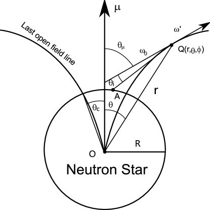
Figure 1: Geometry of the inverse Compton scattering model (Qiao & Lin 1998).

For the geometrical configuration in Figure 1, when the radiation altitudes are far from the pulsar surface, we have (Qiao et al. 2001)

$$\cos\theta_{\rm i}=\frac{2\cos\theta-(R/r)(1-3\cos^{2}\theta)}{\sqrt{(1+3\cos^{2}\theta)[1-2(R/r)\cos\theta+(R/r)^{2}]}}\,,$$ (2)

where $r$ is the distance between the scattering point and the center of the pulsar, $R$ is pulsar radius, $\theta$ is the polar angle between the radiation location and the magnetic axis. For a dipole magnetic field, we have

$$r=R_{\rm e}\sin^{2}\theta\,,$$ (3)

where $R_{\rm e}$ is the maximal radius of a given magnetic field line. The angular beam width $\theta_{\mu}$ of the radiation beam coming from the place with polar angle $\theta$ is,

$$\tan\theta_{\mu}=\frac{3\sin 2\theta}{1+3\cos 2\theta},$$ (4)

where $\theta_{\mu}$ is the angle between the direction of magnetic field at the point Q and the magnetic axis (Figure 1). From the radiation altitude $r$ and Lorentz factor $\gamma$, one can determine the outgoing radio wave frequency $\nu$ and the angular beam width $\theta_{\mu}$ using the above equations.

The energy of the secondary particles decrease as they flow along the field lines, it is usually assumed that the Lorentz factor follows

$$\gamma=\gamma_{0}[1-\xi(r-R)/R_{\rm e}]\,,$$ (5)

where $\gamma_{0}$ is the initial Lorentz factor at the top of the gap and $\xi$ is the energy loss factor. From Equations (1) and (5), one can see that $\nu_{0}$ and $\gamma_{0}$ are degenerated, i.e. different groups of $\nu_{0}$ and $\gamma_{0}$ can give identical results in the ICS model. Thus, in the subsequent test for the ICS model, we fix the value of $\nu_{0}$ without losing generality.

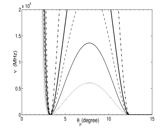
Figure 2: The “beam-frequency mapping” in the ICS model. For the curves from bottom to top, the corresponding $\gamma_{0}$ are 4000, 6000, 8000, 10000, 15000, while $\xi$ is fixed at 50. It shows that $\theta_{\mu}$ at a given frequency in the outer-cone branch becomes insensitive to $\gamma_{0}$ when $\gamma_{0}$ is large enough.

Using the above equations, the relation between the outgoing frequency $\nu$ and the beam width $\theta_{\mu}$, i.e. the function $\nu=\nu(\nu_{0},\gamma_{0},\xi,\theta_{\mu})$, can be calculated. We refer this $\nu$-$\theta_{\mu}$ relation as the “beam-frequency mapping”. A characteristic beam-frequency mapping with the dropping-rising-dropping pattern is given in Figure 2. Compared with the empirical core-double-cone framework for pulsar radiation, the leftmost branch corresponds to the core component, the middle rising part corresponds to the inner cone and the rightmost part corresponds to the outer cone. In this paper, we fit such beam-frequency mapping to the observational data to infer the parameters of ICS model, where the fitting method is given in next section.

3 Method

In our method, we first determine $\theta_{\mu}$ from the pulse width using conventional geometrical model (Gil, 1984; Lyne & Manchester, 1988), and then fit the beam-frequency mapping to $\theta_{\mu}$ data at multiple frequencies to infer the parameters. Here the pulse width $\phi$ is measured using the Gaussian decomposition method (Wu et al. 1992, Kramer et al. 1994a,b, LCW09).

3.1 Measurement of pulse width

The Gaussian decomposition method is widely used to measure the pulse width of a pulse profile, where one models the profile with multiple Gaussian components and extracts the pulse width using curve fitting techniques, i.e. one fits the pulse profile with the following form (Wu et al., 1992; Kramer, 1994; Kramer et al., 1994)

$$I=\sum_{i=1}^{n}I_{i}{\,\rm exp}{\left[-\frac{(\phi-\phi_{i})^{2}}{2\sigma_{i}^{2}}\right]}\,.$$ (6)

Here we denote the intensity of pulse profile $I(\phi)$ as a function of longitudinal phase $\phi$, which is modeled with $n$ Gaussians. The $I_{i}$ is the amplitude of the $i$-th Gaussian, $\phi_{i}$ and $\sigma_{i}$ are the central phase and standard deviation of Gaussian component respectively.

We use the 10% width throughout this paper, which is defined as the full pulse width $2\Delta\phi$ between the leading phase of the leftmost component and the trailing phase of the rightmost component down to the 10% level of their maximal intensities.

The number of Gaussians, the amplitude, the peak phase and the typical width of each Gaussian are free parameters. Following LCW09, we use Levenberg-Marquardt method to perform the least square fitting, which is accepted only when i) nonparametric Kolmogorov-Smirnov test is passed when comparing with the distributions of residues in the on-pulse and off-pulse regions, and ii) the difference between the rms levels of two residues is close to zero, i.e. $\eta=|\sigma_{\rm on}-\sigma_{\rm off}|/\sigma_{\rm off}\simeq 0$. The number of Gaussians is determined by minimizing $\eta$. We run a small Monte-Carlo simulation to determine the final fitting parameters, where the fitting is repeated several times (about 10) with randomly generated initial values, and the final parameters are the averaged values from each individual accepted fitting. We list the measured final pulse width in Table 1.

3.2 Determining angular sizes of radiation beams

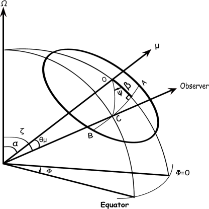
Figure 3: The geometry of pulsar radiation beam. The line of sight sweeps the beam from A to B and the radiation is observed at C (Lyne & Manchester 1988).

From the pulse width, we calculate the angular size of radiation beam following the conventional geometrical model, which assumes that, i) the magnetic field in the magnetosphere is dipolar, and ii) the radiation direction is parallel to the local magnetic field (Figure 3). When the line of sight locates in the $\Omega-\mu$ plane, the rate of linear polarization PA swing reaches the maximum $\kappa$ (Radhakrishnan & Cooke, 1969), where

$$\kappa=\frac{\sin\alpha}{\sin\beta}\,.$$ (7)

Here $\alpha$ is the inclination angle, the impact angle $\beta$ is defined as the angle between the line of sight and the magnetic axis.

Given the inclination angle $\alpha$ and $\kappa$, we can determine $\beta$. We can further substitute $\beta$, $\Delta\phi$ and $\alpha$ into the following geometrical relation to calculate the beam width $\theta_{\rm\mu}$ (Gil, 1984; Lyne & Manchester, 1988)

$$\sin^{2}\left(\frac{\theta_{\mu}}{2}\right)=\sin^{2}\left(\frac{\triangle\phi}{2}\right)\sin\alpha\sin(\alpha+\beta)+\sin^{2}\left(\frac{\beta}{2}\right)\,.$$ (8)

3.3 Measurement for ICS model parameter

The ICS model parameters are derived via fitting the $\theta_{\mu}$ data at multiple frequencies with the beam-frequency mapping. On the one hand, given $N$ frequency bands at central frequencies of $\nu_{i}$, we can measure $N$ beam widths $\theta_{\mu,i}$ from the observation, where $i=1\cdots N$. On the other hand, with Equations (1)-(4), we can calculation the predicted beam width $\theta_{\mu,{\rm i}}^{\rm ics}$ of the ICS model at those frequencies as a function of parameters $\gamma_{0}$ and $\xi$. Thus we can fit the ICS model to the data by minimizing the following standard $\chi^{2}$,

$$\chi^{2}=\sum_{\rm i=1}^{\rm N}\left(\frac{\theta_{\mu,{\rm i}}-\theta_{\mu,{\rm i}}^{\rm ics}}{\delta\theta_{\mu}}\right)^{2}\,,$$ (9)

where $\delta\theta_{\mu}$ is the error of $\theta_{\mu}$. In our fitting, the third ICS model parameter, the background wave frequency $\nu_{0}$, is fixed as $10^{6}$ Hz. Such fixation is due to the parameter degeneracy, i.e. the effect of $\nu_{0}$ is completely absorbed into the parameter $\gamma_{0}$ as indicated in the Equation (1).

4 Data reduction and results

The pulse profile data are from the European Pulsar Network Database, where 15 pulsars are selected according to two criteria, viz. 1) high pulse profile quality at more than five frequencies ranging over one order of magnitude, (2) the absolute values of the maximum slope rate of linear polarization PA $\kappa$ is much larger than 1. The second requirement, i.e. $\kappa\gg 1$, is to make sure that the ratio between angular sizes of radiation beams at different frequencies are insensitive to the inclination angle (Lee et al., 2009).

As explained in the previous section, given the inclination angle $\alpha$, the maximal PA swing slope $\kappa$, and the pulse width, we can calculate the angular sizes $\theta_{\mu}$ of the radiation beams at multiple frequencies. With the beam-frequency mapping, we fit for the ICS model parameters.

One caveat is that it is difficulty to measure the inclination angle accurately. Two types of methods have been used to estimate $\alpha$. The first type of methods are fitting the polarization PA data with the conventional (Radhakrishnan & Cooke, 1969; Lyne & Manchester, 1988; Everett & Weisberg, 2001) or modified versions (Blaskiewicz et al. 1991) of the rotation vector model. The second type of methods are based on some statistical relations between the pulse period and the opening angle of emission beam (Rankin 1990, Kijak & Gil 1997). Due to the limitation of each method and data quality, in many cases, different authors got inconsistent values of inclination angle. Two major methods are used here to reduce the effect of uncertainty of the inclination angle. Firstly, we select pulsars with larger $\kappa$. As proved by LCW09, although the absolute beam width relies on the inclination angle, the ratio between the beam widths at multiple frequencies is insensitive to the inclination angle. Such invariant ratio is already able to determine the ICS model parameters. Secondly, we perform the measurement of $\theta_{\mu}$ and the fitting with the ICS model for all the possible $\alpha$ values, of which the range is presented in Table 2. By enumerate all the possible $\alpha$, we ensure that the invalid parameter space is really not viable.

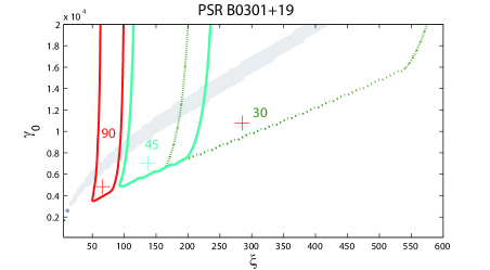
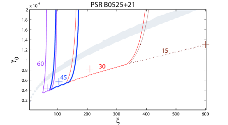
Figure 4: The joint parameter space of the initial Lorentz factor $\gamma_{0}$ and the energy loss factor $\xi$. The grey areas represent the allowed parameter space derived at 95% confidence level through fitting the index of $\theta_{\mu}-\nu$ relation, which is insensitive to inclination angles (LCW09). The solid-line and dotted-line contours represent the 2$\sigma$ confidence regions of $\gamma_{0}$ and $\xi$ constrained by fitting the absolute values of $\theta_{\mu}$ for different inclination angles, where the symbol “+” stands for the best fit $\gamma_{0}$ and $\xi$. For each pulsar, some inclination angles within the possible range given in literature are selected as examples, their values are shown within the contour regions. For a particular inclination angle, the joint parameter space is the overlapped region of grey area and the contour corresponding to the inclination angle. See Table 2 for details of the joint parameter space.

We show the allowed regions in the $\gamma_{0}$–$\xi$ parameter space in Figure 4, where the contours are at 2-$\sigma$ level. We also show the result from the method in LCW09. The results immediately show that fitting the absolute values of $\theta_{\mu}$ can tell us how the allowed parameter space depends on the inclination angle. However, it is not sensitive to constrain $\gamma_{0}$, because the outer-cone branches of beam-frequency curves with the same $\xi$ but different $\gamma_{0}$ are compressed very much along the $\theta_{\mu}$-dimension, as presented in Figure. 2. The constrained parameter ranges are also listed in Table 2. The general features are summarized as follows.

(1) Combining with all the samples, the allowed parameter space are $\gamma_{0}>4000$ and $20<\xi<560$. Since the Lorentz factor of secondary particles is likely well below $10^{5}$ according to inner vacuum gap model, we set the cutoff of $\gamma_{0}$ to be 20000 in calculation. No clear correlation is found between the constrained parameter values and observational quantities, e.g. the pulse width, the surface magnetic field, the pulsar age and the spin-down energy loss rate.

(2) It shows a general trend that both the initial Lorentz factor $\gamma_{0}$ and the energy loss factor $\xi$ increase as $\alpha$ decreases. This is because $\theta_{\mu}$ and the emission altitude $r$ become smaller when $\alpha$ decreases, it requires a faster energy loss so that the Lorentz factor decreases to proper values to produce the radio emission at the observed frequencies.

5 Conclusions and Discussions

We collected a sample of 15 pulsars which have the anti-correlation phenomenon between the pulse width and the observing frequency. Their pulse widths are measured from multi-frequency profiles by using the Gaussian decomposition techniques. Beam widths are calculated with the classical beam geometry model for possible inclination angles. Then they are fitted with the beam-frequency relation of the ICS model to constrain two free parameters, i.e. the initial Lorentz factor $\gamma_{0}$ and the energy loss factor $\xi$. The fitting is performed for a group of possible $\alpha$. It shows a trend that $\gamma_{0}$ and $\xi$ could be larger for smaller inclination angles. The allowed parameter space are $\gamma_{0}>4000$ and $20<\xi<560$. The range of the initial Lorentz factor is generally consistent with the prediction of the inner vacuum gap model (Timokhin 2010). The constrained values of $\xi$ suggest that the secondary particles need to lose a large fraction of their initial energy.

In our calculations, we assume $\nu_{0}=10^{6}$ Hz without losing generality due to the parameter degeneracy, which also agrees with the physical consideration of the inner vacuum gap model. If we take $\nu_{0}=10^{5}$ Hz, according to Equation (1), the resulted Lorentz factors would be about 3 times higher than the present results.

Our results indicates a bit higher Lorentz factor $\gamma_{0}>4000$ than the traditional picture of the inner vacuum gap model ($\sim 1000$ in RS75), but this agrees with the requirement to produce the radio luminosity of pulsars in the ICS model. Noting that the primary particles usually has a Lorentz factor of $10^{6}\sim 10^{7}$ due to radiation reaction (e.g. RS75), the present results imply that the multiplicity of secondary particles is about a few hundred. With such a multiplicity, only a small fraction of secondary particles being coherent (Qiao & Lin 1998) or even incoherent radiation in some cases (Zhang et al. 1999) is sufficient to account for the observed radio luminosity, because the ICS emission of a single particle is much more efficient than the curvature radiation. Harding & Muslimov (2011) found that a slightly asymmetric distortion can significantly increase the accelerating electric field on one side of the polar cap and, combined with a smaller field line radius of curvature, would lead to larger pair multiplicity. This increase of the primary accelerating electric filed may also be the origins of high Lorentz factors of the secondary particles.

The result of $20<\xi<560$ indicates an efficient energy lose for the secondaries. It has been suggested that the resonant inverse Compton scattering between secondaries and thermal photons from the pulsar surface can cause efficient energy loss at a certain surface temperature, but it is only effective within about one stellar radius above the polar cap surface (Zhang et al. 1997, Lyubarskii & Petrova 2000). The other emission mechanisms are much less efficient (Sturner 1995) for secondaries, hence can be neglected. Therefore, the mechanism for such efficient energy loss is still unclear. LCW09 revealed that the decay of secondary Lorentz factor varies significantly from pulsar to pulsar. For some pulsars (e.g. PSR B2016+28), of which the profile width nearly keeps constant at different frequencies, a small value of $\xi$ is thus inferred. Such diversity of energy loss behaviors may due to the interplay between the residual electrical field and the radiation reaction at higher altitudes, of which detailed studies is still demanded.

6 Acknowledgement

We are grateful to the anonymous referee for his/her valuable comments. The work is partially supported by the Bureau of Education of Guangzhou Municipality (No.11 Sui-Jiao-Ke [2009]), GDUPS (2009), Yangcheng Scholar Funded Scheme (10A027S)), NSFC (10778714, 10833003, 10973002, 10821061, 10935001) and the National Basic Research Program of China (Grant 2009CB824800). K. J. Lee is also supported by ERC Grant LEAP , Grant Agreement Number 227947 (PI Michael Kramer).

Table 1: Pulsar parameters and their 10% pulse widths as functions of observing frequencies

Name	$P$ (s)	$B$ ($10^{12}$ G)	$\kappa$	$\nu$ (Hz)	2$\Delta\phi$ (∘)	$\eta$	Reference
B0301+19	1.388	1.36l	-17	0.408	20.2$\pm$3.8	0.206	GL98
				0.61	19.6$\pm$1.1	0.078	GL98
				0.925	18.9$\pm$0.7	0.189	GL98
				1.408	17.7$\pm$0.7	0.133	GL98
				1.642	16.3$\pm$0.5	0.154	GL98
				4.85	15.8$\pm$0.4	0.035	HX97
B0525+21	3.745	12.4	31	0.408	21.7$\pm$1.9	0.031	GL98
				0.61	22.1$\pm$0.7	0.303	GL98
				0.925	21.7$\pm$2.2	0.347	GL98
				1.642	20.9$\pm$0.7	0.458	GL98
				4.85	17.7$\pm$0.6	1.607	HX97
B0540+23	0.246	1.97	-9	0.91	43.2$\pm$2.8	0.068	GL98
				1.408	41.9$\pm$2.0	0.235	GL98
				1.642	43.7$\pm$2.9	0.044	GL98
				4.85	38.8$\pm$1.4	0.069	HX97
				10.45	34.0$\pm$4.0	0.094	HX97
B0823+26	0.531	0.96	-4.5	0.408	21.1$\pm$4.3	0.067	GL98
				0.61	21.2$\pm$2.4	0.369	GL98
				0.925	18.9$\pm$2.5	0.397	GL98
				1.404	12.8$\pm$0.7	0.839	GL98
				4.85	12.7$\pm$1.2	0.727	HX97
				10.55	10.9$\pm$0.3	0.803	SGG95
B0919+06	0.431	2.45	7	0.408	27.9$\pm$1.6	0.290	GL98
				0.61	22.8$\pm$1.5	0.411	GL98
				0.925	17.1$\pm$0.6	0.115	GL98
				1.408	18.8$\pm$1.2	0.070	GL98
				1.642	15.6$\pm$2.4	0.087	GL98
				4.85	10.4$\pm$1.1	0.233	HX97
				10.55	7.6 $\pm$0.3	0.149	SGG95
B1039-19	1.386	1.16	-18	0.4	24.8$\pm$1.3	0.229	ANT94
				0.61	20.3$\pm$0.4	0.394	GL98
				0.8	22.4$\pm$1.0	0.139	ANT94
				0.925	19.5$\pm$1.0	0.230	GL98
				1.408	17.6$\pm$0.5	0.147	GL98
				1.642	18.1$\pm$0.8	0.326	GL98
				4.85	17.6$\pm$1.2	0.032	KKW97
B1133+16	1.188	2.13	12	0.102	22.9$\pm$1.3	1.633	KL99
				0.408	14.7$\pm$0.6	0.095	GL98
				0.925	13.4$\pm$0.7	0.077	GL98
				1.408	14.0$\pm$1.5	0.959	GL98
				1.71	12.3$\pm$0.8	0.614	HX97
				2.25	11.1$\pm$0.4	0.645	KXJ96
				4.85	11.2$\pm$0.6	2.485	HX97
				10.45	9.1$\pm$0.8	0.577	HX97
B1702-19	0.299	1.13	-14	0.61	20.3$\pm$0.7	0.388	GL98
				0.925	18.2$\pm$0.9	0.121	GL98
				1.408	17.4$\pm$0.4	0.437	GL98
				1.642	17.2$\pm$0.4	0.407	GL98
				4.85	16.7$\pm$0.4	0.091	KKW97
B1706-16	0.653	2.05	-9	0.408	14.8$\pm$1.0	0.272	GL98
				0.61	14.2$\pm$0.6	0.251	GL98
				0.925	14.6$\pm$0.8	0.300	GL98
				1.408	14.5$\pm$0.5	0.065	GL98
				4.75	10.8$\pm$0.5	0.103	SGG95
B2020+28	0.343	0.82	15	0.41	18.5$\pm$0.5	0.522	GL98
				0.925	18.5$\pm$0.6	2.365	GL98
				1.408	19.7$\pm$0.4	0.549	GL98
				1.642	19.4$\pm$0.6	1.893	GL98
				4.85	18.6$\pm$0.8	1.780	HX97
				10.45	14.9$\pm$0.7	0.275	HX97
B2021+51	0.529	1.29	4	0.41	25.6$\pm$1.4	0.489	GL98
				0.925	22.3$\pm$0.5	0.788	GL98
				1.408	22.9$\pm$0.8	1.567	GL98
				4.75	17.8$\pm$0.3	0.177	SGG95
				10.45	13.0$\pm$0.4	0.045	HX97
				14.6	12.7$\pm$0.6	0.027	KXJ96
B2045-16	1.962	4.69	-30	0.606	17.8$\pm$0.2	2.131	GL98
				0.925	17.9$\pm$0.8	0.080	GL98
				1.408	16.8$\pm$0.3	1.746	GL98
				1.642	16.4$\pm$0.4	1.788	GL98
				4.85	15.7$\pm$0.5	0.293	HX97
B2154+40	1.525	2.32	8	0.408	32.1$\pm$2.1	0.410	GL98
				0.61	31.4$\pm$0.7	0.294	GL98
				0.925	28.8$\pm$1.4	0.105	GL98
				1.408	29.9$\pm$2.0	0.108	GL98
				1.642	27.4$\pm$1.2	0.191	GL98
				4.85	26.3$\pm$1.2	0.178	HX97
B2310+42	0.349	0.20	4	0.408	19.4$\pm$1.2	0.049	GL98
				0.61	18.4$\pm$0.9	1.417	GL98
				0.925	19.6$\pm$1.1	0.194	GL98
				1.408	17.8$\pm$0.7	1.581	GL98
				1.615	17.6$\pm$0.5	1.419	SGG95
				4.85	15.7$\pm$0.3	0.221	HX97
				10.55	15.2$\pm$0.8	0.127	SGG95
B2319+60	2.256	4.03	-8	0.925	24.7$\pm$0.8	0.079	GL98
				1.408	23.6$\pm$1.0	0.379	GL98
				1.642	22.6$\pm$0.3	0.188	GL98
				4.85	19.8$\pm$0.6	0.146	HX97
				10.55	20.6$\pm$1.4	0.554	SGG95

References. — Pulsar parameters of the periods and the surface magnetic field intensities are taken from ATNF pulsar catalogue (Manchester et al., 1993). The maximal slops of PA curves $\kappa$ are from Lyne & Manchester (1988). The original references for the profile data are given in the last column of the table as the following abbreviations: ANT94-Arzoumanian et al. 1994, GL98-Gould & Lyne 1998, HX97-Hoensbroech & Xilouris 1997, KKW97-Kijak et al. 1997, KL99-Kuz’min & Losovskii 1999, KXJ96-Kramer et al. 1996, SGG95-Seiradakis et al. 1995.

Table 2: Range of the inclination angle $\alpha$ and the constrained joint parameter space.

Name	$\alpha$(∘)	Range of $\xi$	Range of $\gamma_{0}$	References for possible $\alpha$.
B0301+19	5$\sim$90	50$\sim$420	5000$\sim$20000	1 2 3 5 10
B0525+21	14$\sim$67	50$\sim$560	5500$\sim$20000	1 4 5 6 8 9 10
B0540+23	17$\sim$90	10$\sim$90	4000$\sim$16000	1 2 4 8
B0823+26	60$\sim$90	26$\sim$50	5800$\sim$10000	1 2 5 6 9
B0919+06	58$\sim$90	34$\sim$80	4200$\sim$7600	1 8
B1039-19	23$\sim$31	175$\sim$410	11000$\sim$20000	5 10
B1133+16	33$\sim$60	80$\sim$425	6500$\sim$20000	1 5 6 8 9
B1702-19	75	64$\sim$110	10000$\sim$20000	5
B1706-16	40$\sim$70	70$\sim$290	6000$\sim$20000	5 6
B2020+28	60$\sim$71	60$\sim$130	9200$\sim$20000	5 6
B2021+51	16$\sim$30	68$\sim$170	11500$\sim$20000	9
B2045-16	24$\sim$90	70$\sim$375	8000$\sim$20000	2 5
B2154+40	15	210$\sim$430	12000$\sim$20000	5
B2310+42	24$\sim$56	25$\sim$175	4000$\sim$15000	5 6 7
B2319+60	12$\sim$35	85$\sim$245	10800$\sim$20000	5 8

References. — 1-Blaskiewicz et al (1991); 2-Hoensbroech $\&$ Xilouris (1997); 3-Narayan $\&$ Vivekanand (1982); 4-Gould (1994); 5-Kuz’min $\&$ Wu (1992); 6-Lyne $\&$ Manchester (1988); 7-Wang $\&$ Wu (2003); 8-Kijak $\&$ Gil (1997);9-Rankin (1993); 10-Everett $\&$ Weisberg (2001)

References

- Arzoumanian et al. (1994) Arzoumanian, Z., Nice, D.J., Taylor, J.H., & Thorsett, S.E., 1994, ApJ, 422, 671
- Asseo et al. (1990) Asseo, E., Pelletier, G., & Sol, H. 1990, MNRAS, 247, 529
- Bartel Sieber (1978) Bartel, N. & Sieber, W., 1978, A&A, 70, 260
- Blaskiewicz et al. (1991) Blaskiewicz, M., Cordes, J. M., & Wasserman, I. 1991, ApJ, 370, 643
- Everett & Weisberg (2001) Everett, J. E., & Weisberg, J. M. 2001, ApJ, 553, 341
- Gedalin & Melrose (2002) Gedalin, M., Gruman, E., & Melrose, D. B. 2002 MNRAS, 337, 422
- Gil (1984) Gil, J. 1984, A&A, 131, 67
- Gil & Snakowski (1990) Gil, J. A., & Snakowski, J. K. 1990, A&A, 234, 237
- Gould (1994) Gould, D. M. 1994, PhD Thesis, Univ. of Manchester
- Gould & Lyne (1998) Gould, D. M. & Lyne, A. G., 1998, MNRAS, 301, 235
- Harding & Muslimov (2011) Harding, A. K. & Muslimov A. G., 2011, Astrophys. Lett., 726, 10
- Kijak & Gil (1997) Kijak, J., & Gil, J. 1997, MNRAS, 288, 631
- Kijak et al. (1997) Kijak, J., Kramer, M., Wielebinski, R., & Jessner, A., 1997, A&A, 318, 63
- Kramer (1994) Kramer, M. 1994a, A&A, 107, 527
- Kramer et al. (1994) Kramer, M., Wielebinski, R., Jessner, A., Gil, J. A., & Seiradakis, J. H. 1994b, A&A, 107, 515
- Kramer et al. (1996) Kramer, M., Xilouris, K.M., Jessner, A., Lorimer, D.R., Wielebinski, R. & Lyne, A.G., 1996. A&A, 322, 846.
- Kuz’min & Wu (1992) Kuz’min, A. D., & Wu, X. J., 1992, Ap&SS, 190, 209
- Kuz’min & Losovskii (1999) Kuz’min, A. D.; Losovskii, B. Ya., 1999, Astronomy Reports, 43,5
- Lange et al. (1998) Lange, Ch., Kramer, M., Wielebinski, R. & Jessner, A., 1998, A&A, 332, 111
- Lee et al. (2009) Lee, K. J., Cui, X. H., Wang, H. G., Qiao, G. J., & Xu, R. X. 2009, ApJ, 703, 507
- Luo & Melrose (1995) Luo, Q., & Melrose, D. B. 1995, MNRAS, 276, 372
- Lyne & Manchester (1988) Lyne, A. G., & Manchester, R. N. 1988, MNRAS, 234, 477
- Lyubarskii & Petrova (2000) Lyubarskii, Y. E., & Petrova, S. A. 2000, A&A, 355, 406
- Manchester et al. (1993) Manchester, R. N., Hobbs, G. B., Teoh, A. & Hobbs, M., Astron. J.,2005, 129, 1993
- Melrose & Luo (2004) Melrose, D. B., & Luo, Q. 2004, Phys. Rev. E, 70, 6404
- Narayan & Vivekanand (1982) Narayan, R., & Vivekanand, M. 1982, A&A, 113, 3
- Qiao & Lin (1998) Qiao, G. J. , & Lin. W. P. 1998, A&A, 333, 172
- Qiao et al. (2001) Qiao, G. J., Liu, J. F., Zhang, B., & Han, J. L. 2001, A&A, 377, 964
- Radhakrishnan & Cooke (1969) Radhakrishnan, V., & Cooke, D. J. 1969, Astrophys. Lett., 3, 225
- Rankin (1983) Rankin, J. M. 1983a, ApJ, 274, 333
- Rankin (1983) Rankin, J. M. 1983b, ApJ, 274, 359
- Rankin (1990) Rankin, J. M. 1990, ApJ, 352, 247
- Rankin (1993) Rankin, J. M. 1993, ApJS, 85, 145
- Ruderman & Sutherland (1975) Ruderman, M. A., & Sutherland, P. G. 1975, ApJ, 196, 51
- Seiradakis et al. (1995) Seiradakis, J.H., Gil, J.A., Graham, D.A., Jessner, A., Kramer, M., Malofeev, V.M., Sieber, W. & Wielebinski, R., 1995. A&A. Sup. Ser., 111, 205.
- Sturner (1995) Sturner, S. J., 1995, ApJ, 446, 292
- Timokhin (2010) Timokhin, A. N., 2010, MNRAS, 408, 2092
- von Hoensbroech et al. (1997) Hoensbroech, A. V., & Xilouris, K. M. 1997, A&A, 324, 981
- Wang et al. (2003) Wang, H. X., & Wu, X. J. 2003, Chinese J. Astron. Astrophys., 3, 469
- Weatherall (1998) Weatherall, J. C. 1998, ApJ, 506, 341
- Wu et al. (1992) Wu, X. J., Zhang, C. S., Shi, Y. L., & Xu, W. 1992, in Proceedings of Supernovae and Their Remnants, eds: Li Qibin, Ma Er and Li Zongwei, P.113 (International Academic Publishers, 1992)
- Xu et al. (2000) Xu, R. X., Liu, J. F., Han, J. L., & Qiao, G. J. 2000, ApJ, 535, 354
- Zhang et al. (1997) Zhang, B., Qiao, G. J., & Han, J. L., 1997, ApJ, 491, 891
- Zhang et al. (1999) Zhang, B., Hong, B.H., & Qiao, G. J., 1999, Astrophys. Lett., 513, 111
- Zhang et al. (2007) Zhang, H., Qiao, G. J., Han, J. L., Lee, K. J., & Wang, H. G. 2007, A&A, 465, 525