Data compression on the sphere

Large data-sets defined on the sphere arise in many fields. In particular, recent and forthcoming observations of the anisotropies of the cosmic microwave background (CMB) made on the celestial sphere contain approximately three and fifty mega-pixels respectively. The compression of such data is therefore becoming increasingly important. We develop algorithms to compress data defined on the sphere. A Haar wavelet transform on the sphere is used as an energy compression stage to reduce the entropy of the data, followed by Huffman and run-length encoding stages. Lossless and lossy compression algorithms are developed. We evaluate compression performance on simulated CMB data, Earth topography data and environmental illumination maps used in computer graphics. The CMB data can be compressed to approximately 40% of its original size for essentially no loss to the cosmological information content of the data, and to approximately 20% if a small cosmological information loss is tolerated. For the topographic and illumination data compression ratios of approximately 40:1 can be achieved when a small degradation in quality is allowed. We make our SZIP program that implements these compression algorithms available publicly.

1 Introduction

Large data-sets that are measured or defined inherently on the sphere arise in a range of applications. Examples include environmental illumination maps and reflectance functions used in computer graphics (e.g. Ramamoorthi & Hanrahan 2004), astronomical observations made on the celestial sphere, such as the cosmic microwave background (CMB) (e.g. Bennett et al. 1996, 2003), and applications in many other fields, such as planetary science (e.g. Wieczorek 2006; Wieczorek & Phillips 1998; Turcotte et al. 1981), geophysics (e.g. Whaler 1994; Swenson & Wahr 2002; Simons et al. 2006) and quantum chemistry (e.g. Choi et al. 1999; Ritchie & Kemp 1999). Technological advances in observational instrumentation and improvements in computing power are resulting in significant increases in the size of data-sets defined on the sphere (hereafter we refer to a data-set defined on the sphere as a data-sphere). For example, current and forthcoming observations of the anisotropies of the CMB are of considerable size. Recent observations made by the Wilkinson Microwave Anisotropy Probe (WMAP) satellite (Bennett et al., 1996, 2003) contain approximately three mega-pixels, while the forthcoming Planck mission (Planck collaboration, 2005) will generate data-spheres with approximately fifty mega-pixels. Furthermore, cosmological analyses of these data often require the use of Monte Carlo simulations, which generate in the order of a thousand-fold increase in data size. The efficient and accurate compression of data-spheres is therefore becoming increasingly important for both the dissemination and storage of data.

In general, data compression algorithms usually consist of an energy compression stage (often a transform or filtering process), followed by quantisation and entropy encoding stages. For example, JPEG (ISO/IEC IS 10918-1) uses a discrete cosine transform for the energy compression stage, whereas JPEG2000 (ISO/IEC 15444-1:2004) uses a discrete wavelet transform. Due to the simultaneous localisation of signal content in scale and space afforded by a wavelet transform, one would expect wavelet-based energy compression to perform well relative to other methods. Wavelet theory in Euclidean space is well established (see Daubechies (1992) for a detailed introduction), however the same cannot yet be said for wavelet theory on the sphere. A number of attempts have been made to extend wavelets to the sphere. Discrete second generation wavelets on the sphere that are based on a multiresolution analysis have been developed (Schröder & Sweldens, 1995; Sweldens, 1996). Haar wavelets on the sphere for particular pixelisation schemes have also been developed (Tenorio et al., 1999; Barreiro et al., 2000). These discrete constructions allow for the exact reconstruction of a signal from its wavelet coefficients but they may not necessarily lead to a stable basis (see Sweldens (1997) and references therein). Other authors have focused on continuous wavelet methodologies on the sphere (Freeden & Windheuser, 1997; Freeden et al., 1997; Holschneider, 1996; Torrésani, 1995; Dahlke & Maass, 1996; Antoine & Vandergheynst, 1998, 1999; Antoine et al., 2002, 2004; Demanet & Vandergheynst, 2003; Wiaux et al., 2005; Sanz et al., 2006; McEwen et al., 2006). Although signals can be reconstructed exactly from their wavelet coefficients in these continuous methodologies in theory, the absence of an infinite range of dilations precludes exact reconstruction in practice. Approximate reconstruction formula may be developed by building discrete wavelet frames that are based on the continuous methodology (e.g. Bogdanova et al. 2005). More recently, filter bank wavelet methodologies that are essentially based on a continuous wavelet framework have been developed for the axi-symmetric (Starck et al., 2006) and directional (Wiaux et al., 2008) cases. These methodologies allow the exact reconstruction of a signal from its wavelet coefficients in theory and in practice. Compression applications require a wavelet transform on the sphere that allows exact reconstruction, thus the methodologies of Schröder & Sweldens (1995), Tenorio et al. (1999), Barreiro et al. (2000), Starck et al. (2006) and Wiaux et al. (2008) are candidates.

Data compression algorithms on the sphere that use wavelet or alternative transforms have been developed already. Compression on the sphere was considered first, to our knowledge, in the pioneering work of Schröder & Sweldens (1995). The lifting scheme was used here to define a discrete wavelet transform on the sphere, however compression was analysed only in terms of the number of wavelet coefficients required to represent a data-sphere in a lossy manner and no encoding stage was performed. The addition of an encoding stage to this algorithm was performed by Kolarov & Lynch (1997) using zero-tree coding methods. An alternative compression algorithm based on a Faber decomposition has been proposed by Assaf (1999), however no encoding stage is included and performance is again analysed only in terms of the number of coefficients required to recover a lossy representation of the data-sphere. The data-sphere compression algorithm devised by Schröder & Sweldens (1995) and Kolarov & Lynch (1997) therefore constitutes the current state-of-the-art. This algorithm relies on an icosahedron pixelisation of the sphere that is based on triangular subdivisions. The corresponding pixelisation of the sphere precludes pixel centres located on rings of constant latitude. Constant latitude pixelisations of the sphere are of considerable practical use since this property allows the development of many fast algorithms on pixelised spheres, such as fast spherical harmonic transforms. For example, the following constant latitude pixelisations of the sphere have been used extensively in astronomical applications and beyond: the equi-angular pixelisation (Driscoll & Healy, 1994); the Hierarchical Equal Area isoLatitude Pixelisation (HEALPix) (Górski et al., 2005); the IGLOO pixelisation (Crittenden & Turok, 1998); and the GLESP pixelisation (Doroshkevich et al., 2005). Furthermore, at present no data-sphere compression tool is available publicly.

Motivated by the requirement for a data-sphere compression algorithm defined on a constant latitude pixelisation of the sphere, and a publicly available tool to compress such data, we develop wavelet-based compression algorithms for data defined on the HEALPix pixelisation scheme and make our implementation of these algorithms available publicly. We are driven primarily by the need to compress CMB data, hence the adoption of the HEALPix scheme (the pixelisation scheme used currently to store and distribute these data). Wavelet transforms are expected to perform well in the energy compression stage of the compression algorithm, thus we adopt a Haar wavelet transform defined on the sphere for this stage (following a similar framework to that outlined by Barreiro et al. 2000). We could have chosen a filter bank based wavelet framework, such as those developed by Starck et al. (2006) and Wiaux et al. (2008), however, for now, we adopt discrete Haar wavelets due to their simplicity and computational efficiency.

The remainder of this paper is organised as follows. In Sec. 2 we describe the compression algorithms developed, first discussing Haar wavelets on the sphere, before explaining the encoding adopted in our lossless and lossy compression algorithms. The performance of our compression algorithms is then evaluated in Sec. 3. We first examine compression performance for CMB data and study the implications of any errors on cosmological inferences drawn from the data. We then examine compression performance for topographical data and environmental illumination maps. Concluding remarks are made in Sec. 4.

2 Compression algorithms

The wavelet-based compression algorithms that we develop to compress data-spheres consist of a number of stages. Firstly, a Haar wavelet transform is performed to reduce the entropy of the data, followed by quantisation and encoding stages. The resulting algorithm is lossless to numerical precision. We then develop a lossy compression algorithm by introducing an additional thresholding stage, after the wavelet transform, in order to reduce the entropy of the data further. Allowing a small degradation in the quality of decompressed data in this manner improves the compression ratios that may be attained. In this section we first discuss the Haar wavelet transform on the sphere that we adopt, before outlining the subsequent stages of the lossless and lossy compression algorithms. We make our SZIP program that implements these algorithms available publicly. Furthermore, we also provide an SZIP user manual (McEwen & Eyers, 2010), which discusses installation, usage (including a description of all compression options and parameters), and examples.

2.1 Haar wavelets on the sphere

The description of wavelets on the sphere given here is based largely on the generic lifting scheme proposed by Schröder & Sweldens (1995) and also on the specific definition of Haar wavelets on a HEALPix pixelised sphere proposed by Barreiro et al. (2000). However, our discussion and definitions contain a number of notable differences to those given by Barreiro et al. (2000) since we construct an orthonormal Haar basis on the sphere and describe this in a multiresolution setting.

We begin by defining a nested hierarchy of spaces as required for a multiresolution analysis (see Daubechies (1992) for a more detailed discussion of multiresolution analysis). Firstly, consider the approximation space $V_{j}$ on the sphere ${\mathrm{S}^{2}}$, which is a subset of the space of square integrable functions on the sphere, i.e. $V_{j}\subset\mathrm{L}^{2}({\mathrm{S}^{2}})$. One may think of $V_{j}$ as the space of piecewise constant functions on the sphere, where the index $j$ corresponds to the size of the piecewise constant regions. As the resolution index $j$ increases, the size of the piecewise constant regions shrink, until in the limit we recover $\mathrm{L}^{2}({\mathrm{S}^{2}})$ as $j\rightarrow\infty$. If the piecewise constants regions of ${\mathrm{S}^{2}}$ are arranged hierarchically as $j$ increases, then one can construct the nested hierarchy of approximation spaces

$$V_{1}\subset V_{2}\subset\cdots\subset V_{J}\subset\mathrm{L}^{2}({\mathrm{S}^{2}})\>,$$ (1)

where coarser (finer) approximation spaces correspond to a lower (higher) resolution level $j$. For each space $V_{j}$ we define a basis with basis elements given by the scaling functions $\phi_{j,k}\in V_{j}$, where the $k$ index corresponds to a translation on the sphere. Now, let us define $W_{j}$ to be the orthogonal complement of $V_{j}$ in $V_{j+1}$, where the inner product of two square integrable functions on the sphere $f,g\in\mathrm{L}^{2}({\mathrm{S}^{2}})$ is defined by

$$\langle f|g\rangle\equiv\int_{\mathrm{S}^{2}}f(\omega)g^{\ast}(\omega)\mathrm{\,d}\Omega\>,$$

where $\omega=(\theta,\varphi)$ denotes spherical coordinates with colatitude $\theta\in[0,\pi]$ and longitude $\varphi\in[0,2\pi)$, $\ast$ denotes complex conjugation and $\mathrm{\,d}\Omega=\sin\theta\mathrm{\,d}\theta\mathrm{\,d}\varphi$ is the usual rotation invariant measure on the sphere. $W_{j}$ essentially provides a space for the representation of the components of a function in $V_{j+1}$ that cannot be represented in $V_{j}$, i.e. $V_{j+1}=V_{j}\oplus W_{j}$. For each space $W_{j}$ we define a basis with basis elements given by the wavelets $\psi_{j,k}\in W_{j}$. The wavelet space $W_{j}$ encodes the difference (or details) between two successive approximation spaces $V_{j}$ and $V_{j+1}$. By expanding the hierarchy of approximation spaces, the highest level (finest) space $j=J$, can then be represented by the lowest level (coarsest) space $j=1$ and the differences between the approximation spaces that are encoded by the wavelet spaces:

$$V_{J}=V_{1}\oplus\bigoplus_{j=1}^{J-1}W_{j}\>.$$ (2)

Let us now relate the generic description of multiresolution spaces given above to the HEALPix pixelisation. The HEALPix scheme provides a hierarchical pixelisation of the sphere and hence may be used to define the nested hierarchy of approximation spaces explicitly. The piecewise constant regions of the function spaces $V_{j}$ discussed above now correspond to the pixels of the HEALPix pixelisation at the resolution associated with $V_{j}$. To make the association explicit, let $V_{j}$ correspond to a HEALPix pixelised sphere with resolution parameter ${N_{\rm{side}}}=2^{j-1}$ (HEALPix data-spheres are represented by the resolution parameter ${N_{\rm{side}}}$, which is related to the number of pixels in the pixelisation by $N=12{N_{\rm{side}}}^{2}$). In the HEALPix scheme, each pixel at level $j$ is subdivided into four pixels at level $j+1$, and the nested hierarchy given by (1) is satisfied. The number of pixels associated with each space $V_{j}$ is given by $N_{j}=12\times 4^{j-1}$, where the area of each pixel is given by $A_{j}=4\pi/N_{j}=\pi/(3\times 4^{j-1})$ (note that all pixels in a HEALPix data-sphere at resolution $j$ have equal area). It is also useful to note that the number and area of pixels at one level relates to adjacent levels through $N_{j+1}=4N_{j}$ and $A_{j+1}=A_{j}/4$ respectively.

We are now in a position to define the scaling functions and wavelets explicitly for the Haar basis on the nested hierarchy of HEALPix spheres. In this setting the index $k$ corresponds to the position of pixels on the sphere, i.e. for $V_{j}$ we get the range of values $k=0,\cdots,N_{j}-1$, and we let $P_{j,k}$ represent the region of the $k$th pixel of a HEALPix data-sphere at resolution $j$. For the Haar basis, we define the scaling function $\phi_{j,k}$ at level $j$ to be constant for pixel $k$ and zero elsewhere:

$$\phi_{j,k}(\omega)\equiv\begin{cases}1/\sqrt{A_{j}}&\omega\in P_{j,k}\\ 0&\text{elsewhere .}\end{cases}$$

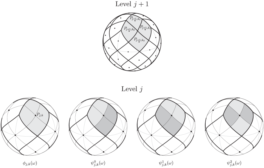
Figure 1: Haar scaling function $\phi_{j,k}(\omega)$ and wavelets $\psi_{j,k}^{m}(\omega)$. Dark shaded regions correspond to negative constant values, light shaded regions correspond to positive constant values and unshaded regions correspond to zero. The scaling function and wavelets at level $j$ and position $k$ are non-zero on pixel $P_{j,k}$ only. Pixel $P_{j,k}$ at level $j$ is subdivided into four pixels at level $j+1$, which we label $P_{j+1,k_{0}}$, $P_{j+1,k_{1}}$, $P_{j+1,k_{2}}$ and $P_{j+1,k_{3}}$ as defined above.

The non-zero value of the scaling function $1/\sqrt{A_{j}}$ is chosen to ensure that the scaling functions $\phi_{j,k}$ for $k=0,\cdots,N_{j}-1$ do indeed define an orthonormal basis for $V_{j}$. Before defining the wavelets explicitly, we fix some additional notation. Pixel $P_{j,k}$ at level $j$ is subdivided into four pixels at level $j+1$, which we label $P_{j+1,k_{0}}$, $P_{j+1,k_{1}}$, $P_{j+1,k_{2}}$ and $P_{j+1,k_{3}}$, as illustrated in Fig. 1. An orthonormal basis for the wavelet space $W_{j}$, the orthogonal complement of $V_{j}$, is then given by the following wavelets of type $m=\{0,1,2\}$:

$$\psi_{j,k}^{0}(\omega)\equiv\bigl{[}\phi_{j+1,k_{0}}(\omega)-\phi_{j+1,k_{1}}(\omega)+\phi_{j+1,k_{2}}(\omega)-\phi_{j+1,k_{3}}(\omega)\bigr{]}/2\>;$$

$$\psi_{j,k}^{1}(\omega)\equiv\bigl{[}\phi_{j+1,k_{0}}(\omega)+\phi_{j+1,k_{1}}(\omega)-\phi_{j+1,k_{2}}(\omega)-\phi_{j+1,k_{3}}(\omega)\bigr{]}/2\>;$$

$$\psi_{j,k}^{2}(\omega)\equiv\bigl{[}\phi_{j+1,k_{0}}(\omega)-\phi_{j+1,k_{1}}(\omega)-\phi_{j+1,k_{2}}(\omega)+\phi_{j+1,k_{3}}(\omega)\bigr{]}/2\>.$$

We require three independent wavelet types to construct a complete basis for $W_{j}$ since the dimension of $V_{j+1}$ (given by $N_{j+1}$) is four times larger than the dimension of $V_{j}$ (the approximation function provides the fourth component). The Haar scaling functions and wavelets defined on the sphere above are illustrated in Fig. 1.

Let us check that the scaling functions and wavelets satisfy the requirements for an orthonormal multiresolution analysis as outlined previously. We require $W_{j}$ to be orthogonal to $V_{j}$, i.e. we require

$$\int_{\mathrm{S}^{2}}\phi_{j,k}(\omega)\psi_{j,k^{\prime}}^{m}(\omega)\mathrm{\,d}\Omega=0\>.$$

This is always satisfied since for $k^{\prime}\neq k$ the scaling function and wavelet do not overlap and so the integrand is zero always, and for $k^{\prime}=k$ we find

$$\int_{\mathrm{S}^{2}}\phi_{j,k}(\omega)\psi_{j,k}^{m}(\omega)\mathrm{\,d}\Omega\propto\int_{\mathrm{S}^{2}}\psi_{j,k}^{m}(\omega)\mathrm{\,d}\Omega=0\>.$$

We also require $W_{j}$ to be orthogonal to $W_{j^{\prime}}$ for all $j$ and $j^{\prime}$. Again, if the basis functions do not overlap (i.e. $k\neq k^{\prime}$) then this requirement is satisfied automatically, and if they do (i.e. $k=k^{\prime}$) then the wavelet at the finer level $j^{\prime}>j$ will always lie within a region of the wavelet at level $j$ with constant value, and consequently

$$\int_{\mathrm{S}^{2}}\psi_{j,k}^{m}(\omega)\psi_{{j^{\prime}},{k^{\prime}}}^{m^{\prime}}(\omega)\mathrm{\,d}\Omega\propto\int_{\mathrm{S}^{2}}\psi_{j^{\prime},k^{\prime}}^{m^{\prime}}(\omega)\mathrm{\,d}\Omega=0\>.$$

Finally, to ensure that we have constructed an orthonormal wavelet basis for $W_{j}$, we check the orthogonality of all wavelets at level $j$:

$$\int_{\mathrm{S}^{2}}\psi_{j,k}^{m}(\omega)\psi_{{j},{k^{\prime}}}^{m^{\prime}}(\omega)\mathrm{\,d}\Omega=\delta_{{m}{m^{\prime}}}\delta_{{k}{k^{\prime}}}\Biggl{(}\frac{1}{2\sqrt{A_{j+1}}}\Biggr{)}^{2}A_{j}=\delta_{{m}{m^{\prime}}}\delta_{{k}{k^{\prime}}}\>,$$

where for $m\neq m^{\prime}$ the positive and negative regions of the integrand cancel exactly and for $k\neq k^{\prime}$ the wavelets do not overlap and so the integrand is zero always. Note that in the previous expression the final $A_{j}$ term arises from the area element $\mathrm{\,d}\Omega$. The Haar approximation and wavelet spaces that we have constructed therefore satisfy the requirements of a orthonormal multiresolution analysis on the sphere. Although the orthogonal nature of these spaces is important, a different normalisation could be chosen. It is now possible to define the analysis and synthesis of a function on the sphere in this Haar wavelet multiresolution framework.

The decomposition of a function defined on a HEALPix data-sphere at resolution $J$, i.e. $f_{J}\in V_{J}$, into its wavelet and scaling coefficients proceeds as follows. Consider an intermediate level $j+1<J$ and let $f_{j+1}$ be the approximation of $f_{J}$ in $V_{j+1}$. The scaling coefficients at the coarser level $j$ are given by the projection of $f_{j+1}$ onto the scaling functions $\phi_{j,k}$:

$$\lambda_{j,k} \equiv\int_{\mathrm{S}^{2}}f_{j+1}(\omega)\phi_{j,k}(\omega)\mathrm{\,d}\Omega$$

$$=\bigl{(}\lambda_{j+1,k_{0}}+\lambda_{j+1,k_{1}}+\lambda_{j+1,k_{2}}+\lambda_{j+1,k_{3}}\bigr{)}\sqrt{A_{j}}/4\>,$$

where we call $\lambda_{j,k}$ the approximation coefficients since they define the approximation function $f_{j}\in V_{j}$. At the finest level $J$, we naturally associate the function values of $f_{J}$ with the approximation coefficients of this level. The wavelet coefficients at level $j$ are given by the projection of $f_{j+1}$ onto the wavelets $\psi_{j,k}^{m}$:

$$\gamma_{j,k}^{m}\equiv\int_{\mathrm{S}^{2}}f_{j+1}(\omega)\psi_{j,k}^{m}(\omega)\mathrm{\,d}\Omega\>,$$

giving

$$\gamma_{j,k}^{0}=\bigl{(}\lambda_{j+1,k_{0}}-\lambda_{j+1,k_{1}}+\lambda_{j+1,k_{2}}-\lambda_{j+1,k_{3}}\bigr{)}\sqrt{A_{j}}/4\>,$$

$$\gamma_{j,k}^{1}=\bigl{(}\lambda_{j+1,k_{0}}+\lambda_{j+1,k_{1}}-\lambda_{j+1,k_{2}}-\lambda_{j+1,k_{3}}\bigr{)}\sqrt{A_{j}}/4\>$$

and

$$\gamma_{j,k}^{2}=\bigl{(}\lambda_{j+1,k_{0}}-\lambda_{j+1,k_{1}}-\lambda_{j+1,k_{2}}+\lambda_{j+1,k_{3}}\bigr{)}\sqrt{A_{j}}/4\>,$$

where we call $\gamma_{j,k}^{m}$ the detail coefficients of type $m$. Starting from the finest level $J$, we compute the approximation and detail coefficients at level $J-1$ as outlined above. We then repeat this procedure to decompose the approximation coefficients at level $J-1$ (i.e. the approximation function $f_{J-1}$), into approximation and detail coefficients at the coarser level $J-2$. Repeating this procedure continually, we recover the multiresolution representation of $f_{J}$ in terms of the coarsest level approximation $f_{1}$ and all of the detail coefficients, as specified by (2) and illustrated in Fig. 2. In general it is not necessary to continue the multiresolution decomposition down to the coarsest level $j=1$; one may choose to stop at the intermediate level $J_{0}$, where $1\leq J_{0}<J$.

The function $f_{J}\in V_{J}$ may then be synthesised from its approximation and detail coefficients. Due to the orthogonal nature of the Haar basis, the approximation coefficients at level $j+1$ may be reconstructed from the weighted expansion of the scaling function and wavelets at the coarser level $j$, where the weights are given by the approximation and detail coefficients respectively. Writing this expansion explicitly, the approximation coefficients at level $j+1$ are given in terms of the approximation and detail coefficients of the coarser level $j$:

$$\lambda_{j+1,k_{0}}=\bigl{(}\lambda_{j,k}+\gamma_{j,k}^{0}+\gamma_{j,k}^{1}+\gamma_{j,k}^{2}\bigr{)}/\sqrt{A_{j}}\>;$$

$$\lambda_{j+1,k_{1}}=\bigl{(}\lambda_{j,k}-\gamma_{j,k}^{0}+\gamma_{j,k}^{1}-\gamma_{j,k}^{2}\bigr{)}/\sqrt{A_{j}}\>;$$

$$\lambda_{j+1,k_{2}}=\bigl{(}\lambda_{j,k}+\gamma_{j,k}^{0}-\gamma_{j,k}^{1}-\gamma_{j,k}^{2}\bigr{)}/\sqrt{A_{j}}\>;$$

$$\lambda_{j+1,k_{3}}=\bigl{(}\lambda_{j,k}-\gamma_{j,k}^{0}-\gamma_{j,k}^{1}+\gamma_{j,k}^{2}\bigr{)}/\sqrt{A_{j}}\>.$$

Repeating this procedure from level $j=J_{0}$ up to $j=J$, one finds that the signal $f_{J}\in V_{J}$ may be written

$$f_{J}(\omega)=\sum_{k=0}^{N_{J_{0}}-1}\lambda_{J_{0},k}\phi_{J_{0},k}(\omega)+\sum_{j=J_{0}}^{J-1}\sum_{k=0}^{N_{j}-1}\sum_{m=0}^{2}\gamma_{j,k}^{m}\psi_{j,k}^{m}(\omega)\>.$$

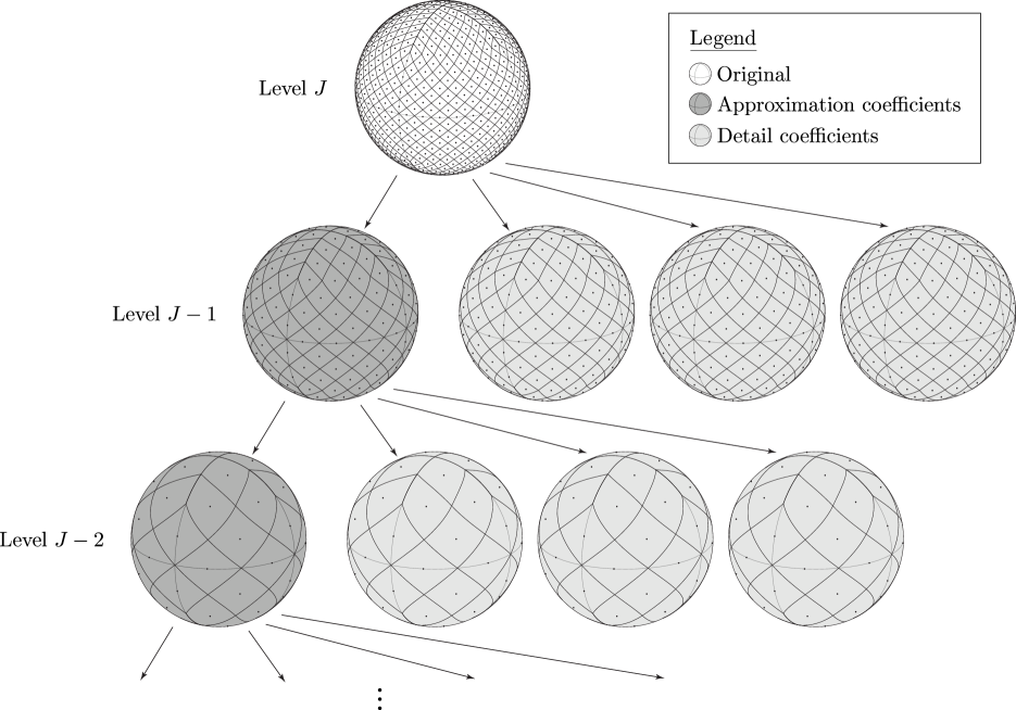
Figure 2: Haar multiresolution decomposition. Starting at the finest level $J$ (the original data-sphere), the approximation and detail coefficients at level $J-1$ are computed. This procedure is repeated to decompose the approximation coefficients at level $J-1$ (i.e. the approximation function $f_{J-1}$), into approximation and detail coefficients at the coarser level $J-2$. Repeating this procedure continually, one recovers the multiresolution representation of $f_{J}$ in terms of the coarsest level approximation $f_{J_{0}}$ and all of the detail coefficients.

2.2 Lossless compression

The Haar wavelet transform on the sphere defined in the previous section is used as the first stage of the lossless compression algorithm. The purpose of this stage is to compress the energy content of the original data. In order to recover the original data from its compressed representation, the energy compression stage must be reversible. This requirement limits candidate wavelet transforms on the sphere to those that allow the exact reconstruction of a signal from its wavelet coefficients. We choose the Haar wavelet transform on the sphere since it satisfies this requirement and also because of its simplicity and computational efficiency.

We demonstrate the energy compression achieved by the Haar wavelet transform with an example. In Fig. 3(a) we show a histogram of the value of each datum contained in a data-sphere that we wish to compress (although the particular data-sphere examined here is not of considerable importance, for the purpose of this demonstration we use the CMB data described in Sec. 3.1). In Fig. 3(b) we show a histogram of the value of the Haar approximation and detail coefficients for the same data-sphere. Notice how the wavelet transform has compressed the energy of the signal so that it is contained predominantly within a smaller range of values. Entropy provides a measure of the information content of a signal and is defined by $H=-\sum_{i}P_{i}\log_{2}P_{i}$, where $P_{i}$ is the probability of symbol $i$ occurring in the data. By compressing the energy of the data so that certain symbols will have higher probability, we reduce its entropy. The aforementioned entropy value also provides a theoretical limit on the best compression of data attainable with entropy encoding, hence by reducing the entropy of data the performance of any subsequent compression is improved.

Following the wavelet transform stage of the compression algorithm, we perform an entropy encoding stage to compress the data. Entropy encoding is a type of variable length encoding, where symbols that occur frequently are given short codewords. The entropy $H$ of the data gives the mean number of bits per datum required to encode the data using an ideal variable length entropy code. We adopt Huffman encoding, which produces a code that closely approximates the performance of the ideal entropy code.

A compression algorithm consisting of the wavelet transform and entropy encoding stages described above would work, however its performance would be limited. Although the wavelet transform compresses the energy of the data, coefficient values that are extremely close to one another may take distinct machine representations. In order to achieve good compression ratios, one requires a compressed energy representation of the data with a relatively small number of unique symbols. To satisfy this requirement we introduce a quantisation stage in our compression algorithm before the Huffman encoding. By quantising we map similar coefficient values to the same machine representation, thus reducing the number of unique symbols contained in the data. The quantisation stage does introduce some distortion and so the resulting compression algorithm is no longer perfectly lossless, but is lossless only to a user specified numerical precision. As one increases the precision parameter, lossless compression is achieved in the limit. The user specified precision parameter $p$ defines the number of significant figures to retain in the wavelet detail coefficients (approximation coefficients are kept to the full number of significant figures provided by the machine representation). The precision parameter trades-off decompression fidelity with compression ratio. The effect of quantisation on compression performance is evaluated in Sec. 3.

For this lossless compression algorithm, data are decompressed simply by decoding the Huffman encoding of the wavelet coefficients, followed by application of the inverse Haar wavelet transform on the sphere.

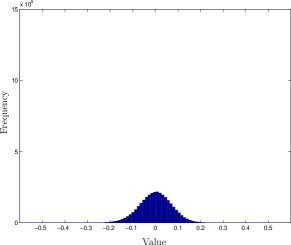
(a) Original data

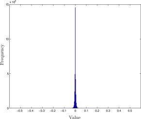
(b) Wavelet coefficients

Figure 3: Histograms of original data and wavelet (approximation and detail) coefficient values. Although the particular data-sphere considered here is not important for the purpose of this demonstration, these histograms correspond to the CMB data described in Sec. 3.1. Notice how the Haar wavelet transform has compressed the energy content of the signal, thereby reducing its entropy and allowing for greater compression performance.

2.3 Lossy compression

If we allow degradation to the quality of the decompressed data it is possible to achieve higher compression ratios. In this section we describe a lossy compression algorithm that trades-off losses in decompression fidelity against compression ratio in a natural manner.

The Haar wavelet representation of a data-sphere decomposes the data into an approximation sphere and detail coefficients that encode the differences between the approximation sphere and the original data-sphere. Many of these detail coefficients are often close to zero (as illustrated by the histogram shown in Fig. 3(b)). If we discard those detail coefficients that are near zero, by essentially setting their value to zero, then we lose only a small amount of accuracy in the representation of the original data but reduce the entropy considerably. By increasing the proportion of detail coefficients neglected, we improve the compression ratio of the compressed data while reducing its fidelity in a natural manner.

Our lossy compression algorithm is identical to the lossless algorithm described in Sec. 2.2 but with two additional stages included. Firstly, we introduce a thresholding stage after the quantisation and before the Huffman encoding stage. The threshold level is determined by choosing the proportion of detail coefficients to retain. We treat the detail coefficients on all levels identically. More sophisticated thresholding algorithms could treat the detail coefficients on each level $j$ differently, perhaps using an annealing scheme to specify the proportion of detail coefficients to retain at each level. However, we demonstrate in Sec. 3.2 that the naïve thresholding scheme outlined here performs very well in practice and so we do not investigate more sophisticated strategies. Once the threshold level is determined we perform hard thresholding so that all detail coefficients below this value are set to zero, while coefficients above the threshold remain unaltered. The thresholding stage reduces the number of unique symbols in the data by replacing many unique values with zero, hence reducing the entropy of the data and enabling greater compression. Furthermore, since many of the data are now zero, it is worthwhile to incorporate a run length encoding (RLE) stage so that long runs of zeros are encoded efficiently. The RLE stage is included after the thresholding and before the Huffman encoding stage. RLE introduces some additional encoding overhead, thus it only improves the compression ratio for cases where there are sufficiently long runs of zeros. In Sec. 3.2 we evaluate the performance of the lossy compression algorithm described here and examine the trade-off between compression ratio and fidelity. Moreover, we also examine cases where the additional overhead due to RLE acts to increase the compression ratio.

For this lossy compression algorithm, data are decompressed simply by decoding the RLE and Huffman encoding of the wavelet coefficients, followed by application of the inverse Haar wavelet transform on the sphere.

3 Applications

In this section we evaluate the performance of the lossless and lossy compression algorithms on data-spheres that arise in a range of applications. The trade-off between compression ratio and the fidelity of the decompressed data is examined in detail. We begin by considering applications where lossless compression is required, before then considering applications when lossy compression is appropriate.

3.1 Lossless compression

The algorithms developed here to compress data defined on the sphere were driven primarily by the need to compress large CMB data-spheres. CMB data are used to study cosmological models of the Universe. Any errors introduced in the data may alter cosmological inferences drawn from it, hence the introduction of large errors in the compression of CMB data will not be tolerated. The lossless compression algorithm is therefore required for this application. Our lossless compression algorithm is lossless only to a user specified numerical precision (as described in detail in Sec. 2.2). It is therefore important to ascertain whether the small quantisation errors that are introduced by this limited precision could affect cosmological inferences drawn from the data. We first evaluate the performance of the lossless compression of CMB data, before investigating the impact of errors on the cosmological information content of the data.

To evaluate our lossless compression algorithm we use simulated CMB data. In the simplest inflationary models of the Universe, the CMB is fully described by its angular power spectrum. Using the theoretical angular power spectrum that best fits the three-year WMAP observations (i.e. the power spectrum defined by the cosmological parameters specified in Table 2 of Spergel et al. (2007)), we simulate a Gaussian realisation of the CMB temperature anisotropies. Foreground emissions contaminate real observations of the CMB, hence we also consider simulated maps where a mask is applied to remove regions of known Galactic and point source contamination. We apply the conservative Kp0 mask associated with the three-year WMAP observations (Hinshaw et al., 2007). These simulated CMB data, with and without application of the Kp0 mask, are illustrated at resolutions ${N_{\rm{side}}}=512$ ($J=9$; $N\simeq 3\times 10^{6}$) and ${N_{\rm{side}}}=1024$ ($J=10$; $N\simeq 13\times 10^{6}$) in the first column of panels of Fig. 4.

The simulated CMB data are compressed using the lossless compression algorithm for a range of precision values $p$. RLE is applied when compressing the masked data to efficiently compress the runs of zeros associated with the masked regions but not for the unmasked data (since the encoding overhead does not make it worthwhile). For each precision value, we compute the compression ratio achieved and the relative error between the decompressed data and the original data. The compression ratio is defined by the ratio of the size of the compressed data (including the Huffman encoding table) relative to the size of the original data, expressed as a percentage. The error used to evaluate the fidelity of the compressed data is defined by the ratio of the mean-square-error (MSE) between the original and decompressed data-spheres relative to the root-mean-squared (RMS) value of the original data-sphere, expressed as a percentage. These values are plotted for a range of precision values in the third column of panels of Fig. 4. In the second column of panels of Fig. 4 residual errors between the original data and decompressed data reconstructed for a precision parameter $p=3$ are shown, where a compression ratio of 18% is achieved for resolution ${N_{\rm{side}}}=1024$. Although the precision level $p=3$ introduces some error in the reconstructed data (2.7% for ${N_{\rm{side}}}=1024$), the error on each pixel is reassuringly small at typically a factor of $\sim 100$ smaller than the corresponding data value. For the precision parameter $p=5$, a compression ratio of 40% and an error of 0.03% is obtained for resolution ${N_{\rm{side}}}=1024$. The error introduced by the compression for this case is sufficiently small that one might hope that no significant cosmological information content is lost in the compressed data. We investigate the cosmological information content of the compressed data in detail next.

 
 
   

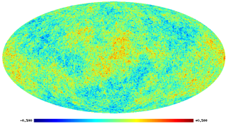
(a) CMB at ${N_{\rm{side}}}=512$ (13MB)

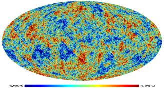
(b) Residual for $p=3$ at ${N_{\rm{side}}}=512$ (2.5MB)

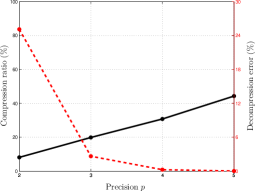
(c) Performance at ${N_{\rm{side}}}=512$

(d) Masked CMB at ${N_{\rm{side}}}=512$ (13MB)

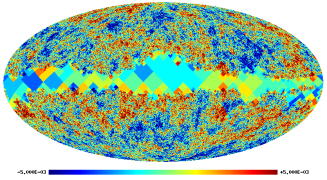
(e) Masked residual for $p=3$ at ${N_{\rm{side}}}=512$ (2.1MB)

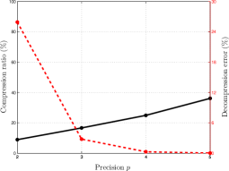
(f) Masked performance at ${N_{\rm{side}}}=512$

(g) CMB at ${N_{\rm{side}}}=1024$ (50MB)

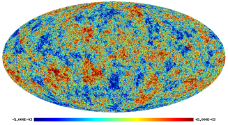
(h) Residual for $p=3$ at ${N_{\rm{side}}}=1024$ (9.1MB)

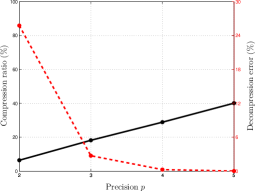
(i) Performance at ${N_{\rm{side}}}=1024$

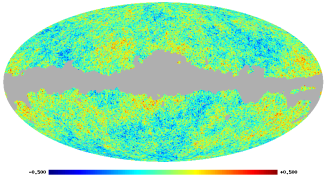
(j) Masked CMB at ${N_{\rm{side}}}=1024$ (50MB)

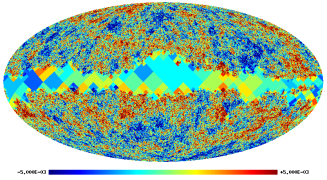
(k) Masked residual for $p=3$ at ${N_{\rm{side}}}=1024$ (7.6MB)

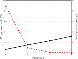
(l) Masked performance at ${N_{\rm{side}}}=1024$

Figure 4: Lossless compression of simulated Gaussian CMB data, with and without application of the Kp0 mask (data-spheres are displayed using the Mollweide projection). The first column of panels shows the original simulated CMB data, with corresponding file sizes also specified. The second column of panels shows the residual of the original and decompressed CMB data reconstructed for a precision parameter of $p=3$, with corresponding file sizes of the compressed data also specified. Note that the colour scale between the first and second column of panels is scaled by a factor of 100. RLE is applied when compressing the masked data to efficiently compress the runs of zeros associated with the masked regions. The third column of panels shows the trade-off between compression ratio and decompression fidelity with precision parameter $p$. Compression ratio (solid black line; left axis) is defined by the ratio of the compressed file size relative to the original file size, expressed as a percentage. The decompression error (dashed red line; right axis) is defined by the ratio of the MSE between the original and decompressed data relative to the RMS value of the original data, expressed as a percentage.

In the simplest inflationary scenarios the cosmological information content of the CMB is contained fully in its angular power spectrum. Although the angular power spectrum does not contain all cosmological information in non-standard inflationary settings, anisotropic models of the Universe or various cosmic defect scenarios, we nevertheless use it as a figure of merit to determine any errors in the cosmological information content of CMB data. To evaluate any loss to the cosmological information content of compressed CMB data, we examine the errors that are induced in the angular power spectrum of the compressed data. We consider here unmasked CMB data only, which simplifies the estimation of the angular power spectrum. Before proceeding, we briefly define the angular power spectrum of the CMB and the estimator that we use to compute the power spectrum from CMB data. The angular power spectrum $C_{\ell}$ is given by the variance of the spherical harmonic coefficients of the CMB, i.e. $\langle a_{\ell m}a_{\ell m}^{\ast}\rangle=C_{\ell}\delta_{{\ell}{\ell^{\prime}}}\delta_{{m}{m^{\prime}}}$, where $\delta_{{i}{j}}$ is the Kronecker delta symbol and the spherical harmonic coefficients $a_{\ell m}$ are given by the projection of the CMB anisotropies $\Delta T(\theta,\varphi)$ onto the spherical harmonic functions $Y_{\ell m}(\theta,\varphi)$ through $a_{\ell m}=\langle\Delta T|Y_{\ell m}\rangle$. If the CMB is assumed to be isotropic, then for a given $\ell$ the $m$-modes of the spherical harmonic coefficients are independent and identically distributed. The underlying $C_{\ell}$ spectrum may therefore be estimated by the quantity $\hat{C}_{\ell}\equiv\sum_{m=-\ell}^{\ell}|a_{\ell m}|/(2\ell+1)$. Since more $m$-modes are available at higher $\ell$, the error on this estimator reduces as $\ell$ increases. This phenomenon is termed cosmic variance and arises since we may observe one realisation of the CMB only. Cosmic variance is given by $(\Delta\hat{C}_{\ell})^{2}=2C_{\ell}^{2}/(2\ell+1)$ and provides a natural uncertainty level for power spectrum estimates made from CMB data. Any errors introduced in the angular power spectrum of compressed CMB data may therefore be related to cosmic variance to determine the cosmological implication of these errors. In Fig. 5 we show the angular power spectrum computed for the original and compressed CMB data for ${N_{\rm{side}}}=1024$, and errors between these spectra, for a range of precision parameter values. In the first two columns of panels we also highlight the three standard deviation confidence interval due to cosmic variance. For the precision parameter $p=5$, we find that essentially no cosmological information content is lost in the compressed data. Even for large values of $\ell$, for which cosmic variance is very small, the error in the recovered power spectrum relative to cosmic variance is of the order of a few percent only. For the case $p=4$, still only minimal cosmological information content is lost, while for the case $p=3$ we begin to see a moderate loss of cosmological information. Obviously the degree of cosmological information content loss that may be tolerated depends on the application at hand. However, we have demonstrated that it is possible to compress CMB data to 40% of its original size while ensuring that essentially no cosmological information content is lost (corresponding to $p=5$). If one tolerates a moderate loss of cosmological information then the data may be compressed to 18% of its original size (corresponding to $p=3$).

     

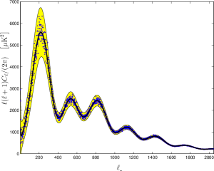
(a) Angular power spectra for $p=5$

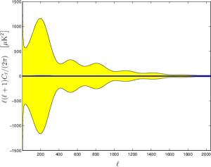
(b) Absolute error for $p=5$

(c) Error relative to cosmic variance for $p=5$

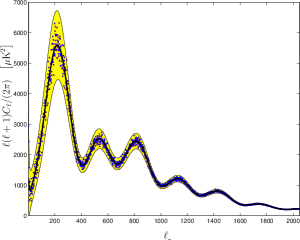
(d) Angular power spectra for $p=4$

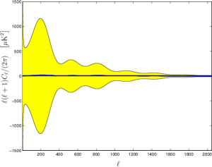
(e) Absolute error for $p=4$

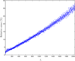
(f) Error relative to cosmic variance for $p=4$

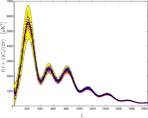
(g) Angular power spectra for $p=3$

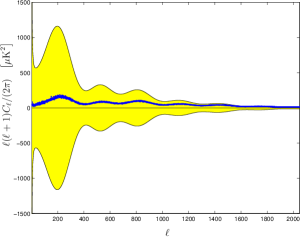
(h) Absolute error for $p=3$

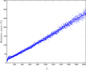
(i) Error relative to cosmic variance for $p=3$

Figure 5: Reconstructed angular power spectrum of compressed CMB data at resolution ${N_{\rm{side}}}=1024$. Each row of panels shows the reconstructed power spectrum and errors for a particular compression precision parameter $p$. In the first column of panels, the power spectrum reconstructed from the original CMB data are given by the red dots, the power spectrum reconstructed from the compressed CMB data are given by the blue dots and the underlying power spectrum of the simulated model is shown by the solid black line, with three standard deviation cosmic variance regions shaded in yellow. Note that in some instances the red and blue dots align closely and may not both be visible. In the second column of panels, the absolute error between the power spectra reconstructed from the original and compressed CMB data is given by the blue dots, with three standard deviation cosmic variance regions shaded in yellow. In the third column of panels, the absolute error between the power spectra reconstructed from the original and compressed CMB data is expressed as a percentage of cosmic variance. Note that the scale of the vertical axis changes by an order of magnitude between each row of the third column of panels.

Finally, we measure the CPU time required to compress and decompress CMB maps. All timing tests are performed on a laptop with a 2.66GHz Intel Core 2 Duo processor and 4GiB of RAM. We restrict our attention to unmasked data and to precision parameters $p=3$ and $p=5$ only. Computation times are plotted in Fig. 6 for a range of resolutions, where all measurements are averaged over five random Gaussian CMB simulations. Note that computation time increases with precision parameter $p$ since the number of unique wavelet coefficients requiring encoding also increases with $p$. All stages of our compression and decompression algorithms are linear in the number of data samples, hence the computation time of our algorithms scales linearly with the number of samples on the sphere, i.e. as $\mathcal{O}({N_{\rm{side}}}^{2})$, as also apparent from Fig. 6.

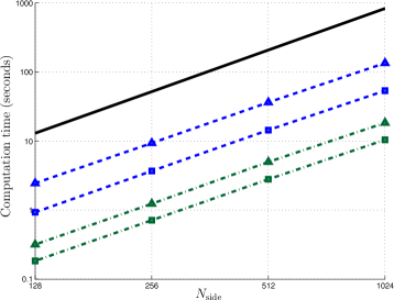
Figure 6: Computation time required to compress (blue/dashed line) and decompress (green/dot-dashed line) simulated Gaussian CMB data of various resolution ${N_{\rm{side}}}$. Computation times are averaged over five simulated Gaussian CMB maps and are shown for precisions parameters $p=3$ (squares) and $p=5$ (triangles). $\mathcal{O}({N_{\rm{side}}}^{2})$ scaling is shown by the heavy black/solid line.

3.2 Lossy compression

In certain applications the loss of a small amount of information from a data-sphere is not catastrophic. For example, in computer graphics environmental illumination maps and reflectance functions that are defined on the sphere are used in rendering synthetic images (e.g. Ramamoorthi & Hanrahan 2004). In this application accuracy is determined by human perception, hence errors may be tolerated if they are not suitably noticeable. Moreover, data-spheres that are input to reflectance algorithms are not viewed directly, thus moderate errors in these data may not necessarily produce noticeable errors in rendered images. Lossy representations of data-spheres in computer graphics are therefore not only tolerated, but are often desired as they may improve the computational efficiency of rendering algorithms (e.g. Ng et al. 2004). For data compression purposes, our lossy compression algorithm is certainly appropriate and may be applied in order to achieve higher compression ratios. In addition to the environmental illumination maps discussed previously, we also compress Earth topography data and evaluate the performance of both our lossless and lossy compression algorithms on both of these types of data.

The Earth topography and environmental illumination data-spheres considered here are all obtained from real-world observations. The original data are illustrated in the first column of panels in Fig. 7. The topographical data are represented at a HEALPix resolution of ${N_{\rm{side}}}=512$. The environmental illumination data-spheres were constructed by Debevec (1998) and are available publicly. These data defined on the sphere were constructed by taking two photographic images of a mirrored ball from different locations, and mapping the observed intensities of the images onto the surface of a sphere. The illumination maps are available in a cross-cube format and have been converted to a HEALPix data-sphere at resolution ${N_{\rm{side}}}=256$ ($J=8$; $N\simeq 0.8\times 10^{6}$). We consider environmental illumination data that was captured in this manner from within Galileo’s Tomb in Santa Croce, Florence, St. Peter’s Basilica in Rome and the Uffizi Gallery in Florence.

Lossless and lossy compressed versions of the data are illustrated in Fig. 7. For the lossless compression we use a precision parameter of $p=3$ in the quantisation stage of the compression since ultimately we are concerned with achieving a high compression ratio and will allow some quantisation error. For the lossy compression we again use a precision parameter of $p=3$ and retain only 5% of the detail coefficients in the thresholding stage of the compression algorithm. Compression ratios of approximately 40:1 are achieved for the lossy compression of both the topographic and environmental illumination data. Although it is possible to discern errors in the lossy compressed data, the overall structure and many of the details of the original data are well approximated in this highly compressed representation.

               

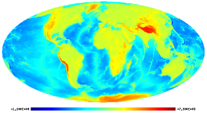
(a) Earth: original (13MB)

(b) Earth: lossless compressed (1.4MB)

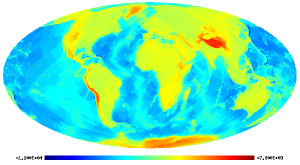
(c) Earth: lossy compressed (0.33MB)

(d) Galileo: original (3.2MB)

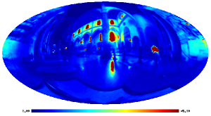
(e) Galileo: lossless compressed (0.21MB)

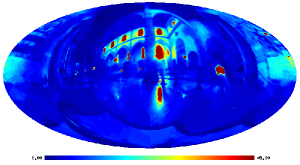
(f) Galileo: lossy compressed (0.07MB)

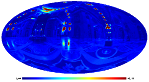
(g) St Peter’s: original (3.2MB)

(h) St Peter’s: lossless compressed (0.20MB)

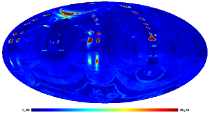
(i) St Peter’s: lossy compressed (0.08MB)

(j) Uffizi: original (3.2MB)

(k) Uffizi: lossless compressed (0.19MB)

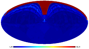
(l) Uffizi: lossy compressed (0.10MB)

Figure 7: Compressed data for lossy compression applications (data-spheres are displayed using the Mollweide projection). Each row of panels shows the original, lossless and lossy compressed data-spheres. File sizes for each data-sphere are also specified. The lossless compressed data shown in the second column of panels is performed with a precision parameter of $p=3$. The lossy compressed data shown in the third column of panels is performed by retaining 5% of detail coefficients only and including a RLE stage. The full dynamic range of these images may not be visible in printed versions of this figure, hence this figure is best viewed online.

In Fig. 8 we evaluate the performance of the compression of these data more thoroughly. Firstly, for the lossless compression we examine the trade-off between compression ratio and decompression error with respect to the precision parameter $p$ (see the first column of panels of Fig. 8). For both the topographic and illumination data it is apparent that we may reduce the precision parameter to $p=3$, while introducing quantisation error on the order of a few percent only. If the precision parameter is reduced to $p=2$, quantisation errors on the order of 10-20% appear. We therefore choose $p=3$ for the lossless compression since this maximises the compression ratio while introducing an allowable level of quantisation error. We then examine the effect of increasing the threshold level, by reducing the proportion of detail coefficients retained, on the performance of the lossy compression (see the second column of panels of Fig. 8). Retaining 100% of the detail coefficients corresponds to the lossless compression case, where no RLE is included. RLE is included for all other lossy compression cases. Notice that when retaining 50% of the detail coefficients, the resulting improvement to the compression ratio is offset by the additional encoding overhead of the RLE. Consequently, the compression ratio when retaining 50% of coefficients (with RLE) is often worse than when retaining 100% of coefficients (without RLE). As the proportion of detail coefficients that are retained is reduced, the improvement to compression ratio quickly exceeds the additional overhead of RLE. Decompression error remains at approximately 5% when retaining only 5% of the detail coefficients, but increases quickly as the proportion of coefficients retained is reduced further. Retaining 5% of coefficients therefore appears to give a good trade-off between compression ratio and fidelity of the decompressed data, justifying this choice for the results presented in Fig. 7. For this choice, the topographic and illumination data are compressed to a ratio of approximately 40:1, while introducing errors of approximately 5%. The images illustrated in Fig. 7 show that errors of this order are not significantly noticeable and are likely to be acceptable for many applications. Also notice that the curves shown in Fig. 8 for the environmental illumination data are similar, indicating that the characteristics of natural illumination are to some extent independent of the scene. One would therefore expect the compression performance observed for the data-spheres considered here to be typical of environmental illumination data in general. Although we have made a number of arbitrary choices here regarding acceptable levels of distortion in the decompressed data, one may of course choose the number of detail coefficients retained that provides a trade-off between compression ratio and fidelity that is suitable for the application at hand.

  
  
  
  

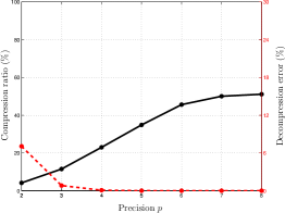
(a) Earth: lossless performance

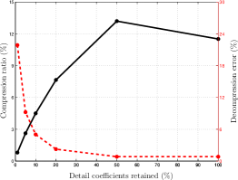
(b) Earth: lossy performance

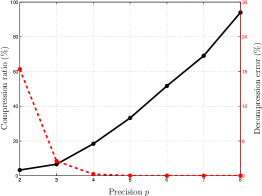
(c) Galileo: lossless performance

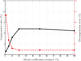
(d) Galileo: lossy performance

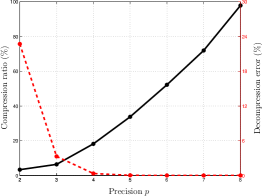
(e) St Peter’s: lossless performance

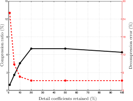
(f) St Peter’s: lossy performance

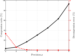
(g) Uffizi: lossless performance

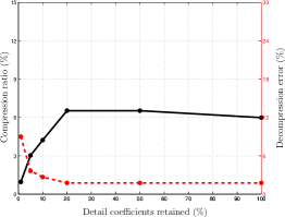
(h) Uffizi: lossy performance

Figure 8: Compression performance for lossy compression applications. Each row of panel shows performance plots for various data-spheres. The first column of panels shows the trade-off between compression ratio and decompression fidelity with precision parameter $p$ for lossless compression. The second column of panels shows the same trade-off, but with respect to the number of detail coefficients retained in the lossy compression. A precision parameter of $p=3$ is used for all lossy compression results illustrated here. Compression ratio (solid black line; left axis) and decompression error (dashed red line; right axis) are defined in the caption of Fig. 4.

4 Concluding remarks

We have developed algorithms to preform lossless and lossy compression of data defined on the sphere. These algorithms adopt a Haar wavelet transform on the sphere to compress the energy content of the data, prior to quantisation and Huffman encoding stages. Note that the resulting lossless compression algorithm is lossless to a user specified numerical precision only. The lossy compression algorithm incorporates, in addition, a thresholding stage so that only a user specified proportion of detail coefficients are retained, and a RLE stage. By allowing a small degradation to the fidelity of the compressed data in this manner, significantly greater compression ratios can be attained.

The performance of these compression algorithms has been evaluated on a number of data-spheres and the trade-off between compression ratio and the fidelity of the decompressed data has been examined thoroughly. Firstly, the lossless compression of CMB data was performed and it was demonstrated that the data can be compressed to 40% of their original size, while ensuring that essentially none of the cosmological information content of the data is lost. A compression ratio of approximately 20% can be achieved if a small loss of cosmological information is tolerated. Secondly, the lossy compression of Earth topography and environmental illumination data was performed. For both of these data types compression ratios of approximately 40:1 can be achieved, while introducing relative errors of approximately 5%. By taking account of the geometry of the sphere that these data live on, we achieve superior compression performance than naïvely applying standard compression algorithms to the data (such as a JPEG compression of the six planes of a cross-cube representation of a data-sphere, for example). On inspection of the decompressed data, it is possible to discern errors in the recovered data by eye, nevertheless the overall structure and many of the details of the data are well approximated. The accuracy of the compressed data remains suitable for many applications.

A number of avenues exist to improve the performance of the current compression algorithms. We choose Haar wavelets on the sphere for the energy compression stage due to their simplicity and computational efficiency. However, the scale discretised wavelet methodology developed by Wiaux et al. (2008) may yield better compression performance due to the ability to represent directional structure in the original data efficiently. However, this wavelet transform is computed in spherical harmonic space; forward and inverse spherical harmonic transforms are not exact on a HEALPix pixelisation. Consequently, greater errors will be introduced in any compression strategy based on this transform. For alternative constant latitude pixelisations of the sphere, however, exact (and fast) spherical harmonic transforms do exist and could be adopted (McEwen & Wiaux, 2011). Nevertheless, the implementation of the scale discretised wavelet is also considerably more demanding computationally. Scope also remains to improve the lossy compression algorithm by treating the detail coefficients at each level differently, perhaps by using an annealing scheme to dynamically specify the proportion of detail coefficients to retain at each level. Nevertheless, the naïve thresholding strategy adopted currently has been demonstrated to perform very well.

The algorithms that we have developed to compress data defined on the sphere have been demonstrated to perform well and we hope that our publicly available implementation will now find practical use. Obviously these compression algorithms may be used to reduce the storage and dissemination costs of data defined on the sphere, but the compressed representation of data-spheres may also find use in the development of fast algorithms that exploit this representation (e.g. Ng et al. 2004). Furthermore, data defined on other two-dimensional manifolds may be compressed by first mapping these data to a sphere, before applying our data-sphere compression algorithms. We are currently pursuing this idea for the compression of three-dimensional meshes used to represent computer graphics models.

References

- Antoine et al. (2002) Antoine J.P., Demanet L., Jacques L., Vandergheynst P., 2002, Applied Comput. Harm. Anal., 13, 3, 177
- Antoine et al. (2004) Antoine J.P., Murenzi R., Vandergheynst P., Ali S.T., 2004, Two-Dimensional Wavelets and their Relatives, Cambridge University Press, Cambridge
- Antoine & Vandergheynst (1998) Antoine J.P., Vandergheynst P., 1998, J. Math. Phys., 39, 8, 3987
- Antoine & Vandergheynst (1999) Antoine J.P., Vandergheynst P., 1999, Applied Comput. Harm. Anal., 7, 1
- Assaf (1999) Assaf D., 1999, Data compression on the sphere using faber decomposition
- Barreiro et al. (2000) Barreiro R.B., Hobson M.P., Lasenby A.N., Banday A.J., Górski K.M., Hinshaw G., 2000, Mon. Not. Roy. Astron. Soc., 318, 475, \hrefhttp://arXiv.org/abs/astro-ph/0004202astro-ph/0004202
- Bennett et al. (1996) Bennett C.L., et al., 1996, Astrophys. J. Lett., 464, 1, 1, \hrefhttp://arXiv.org/abs/astro-ph/9601067astro-ph/9601067
- Bennett et al. (2003) Bennett C.L., et al., 2003, Astrophys. J. Supp., 148, 1, \hrefhttp://arXiv.org/abs/astro-ph/0302207astro-ph/0302207
- Bogdanova et al. (2005) Bogdanova I., Vandergheynst P., Antoine J.P., Jacques L., Morvidone M., 2005, Applied Comput. Harm. Anal., 19, 2, 223
- Choi et al. (1999) Choi C.H., Ivanic J., Gordon M.S., Ruedenberg K., 1999, J. Chem. Phys., 111, 19, 8825
- Crittenden & Turok (1998) Crittenden R.G., Turok N.G., 1998, ArXiv, \hrefhttp://arXiv.org/abs/astro-ph/9806374astro-ph/9806374
- Dahlke & Maass (1996) Dahlke S., Maass P., 1996, J. Fourier Anal. and Appl., 2, 379
- Daubechies (1992) Daubechies I., 1992, Ten Lectures on Wavelets, CBMS-NSF Reg. Conf. Series in Applied Math., SIAM, Philadelphia
- Debevec (1998) Debevec P., 1998, Computer Graphics, 32, Annual Conference Series, 189
- Demanet & Vandergheynst (2003) Demanet L., Vandergheynst P., 2003, in Proc. SPIE, volume 5207, 208–215
- Doroshkevich et al. (2005) Doroshkevich A.G., Naselsky P.D., Verkhodanov O.V., Novikov D.I., Turchaninov V.I., Novikov I.D., Christensen P.R., Chiang L.Y., 2005, Int. J. Mod. Phys. D., 14, 2, 275, \hrefhttp://arXiv.org/abs/astro-ph/0305537astro-ph/0305537
- Driscoll & Healy (1994) Driscoll J.R., Healy D.M.J., 1994, Advances in Applied Mathematics, 15, 202
- Freeden et al. (1997) Freeden W., Gervens T., Schreiner M., 1997, Constructive approximation on the sphere: with application to geomathematics, Clarendon Press, Oxford
- Freeden & Windheuser (1997) Freeden W., Windheuser U., 1997, Applied Comput. Harm. Anal., 4, 1
- Górski et al. (2005) Górski K.M., Hivon E., Banday A.J., Wandelt B.D., Hansen F.K., Reinecke M., Bartelmann M., 2005, Astrophys. J., 622, 759, \hrefhttp://arXiv.org/abs/astro-ph/0409513astro-ph/0409513
- Hinshaw et al. (2007) Hinshaw G., et al., 2007, Astrophys. J. Supp., 170, 288, \hrefhttp://arXiv.org/abs/astro-ph/0603451astro-ph/0603451
- Holschneider (1996) Holschneider M., 1996, J. Math. Phys., 37, 4156
- Kolarov & Lynch (1997) Kolarov K., Lynch W., 1997, in J. Storer, M. Cohn, editors, Data Compression Conference, IEEE Computer Society Press, 281–291
- McEwen & Eyers (2010) McEwen J.D., Eyers D.M., 2010, SZIP user manual, Technical report, University of Cambridge
- McEwen et al. (2006) McEwen J.D., Hobson M.P., Lasenby A.N., 2006, ArXiv, \hrefhttp://arXiv.org/abs/astro-ph/0609159astro-ph/0609159
- McEwen & Wiaux (2011) McEwen J.D., Wiaux Y., 2011, IEEE Trans. Sig. Proc., submitted
- Ng et al. (2004) Ng R., Ramamoorthi R., Hanrahan P., 2004, ACM Transactions on Graphics, 477
- Planck collaboration (2005) Planck collaboration, 2005, ESA Planck blue book, Technical Report ESA-SCI(2005)1, ESA, \hrefhttp://arXiv.org/abs/astro-ph/0604069astro-ph/0604069
- Ramamoorthi & Hanrahan (2004) Ramamoorthi R., Hanrahan P., 2004, ACM Transactions on Graphics, 23, 4, 1004
- Ritchie & Kemp (1999) Ritchie D.W., Kemp G.J.L., 1999, J. Comput. Chem., 20, 4, 383
- Sanz et al. (2006) Sanz J.L., Herranz D., López-Caniego M., Argüeso F., 2006, in EUSIPCO, \hrefhttp://arXiv.org/abs/astro-ph/0609351astro-ph/0609351
- Schröder & Sweldens (1995) Schröder P., Sweldens W., 1995, in Computer Graphics Proceedings (SIGGRAPH ‘95), 161–172
- Simons et al. (2006) Simons F.J., Dahlen F.A., Wieczorek M.A., 2006, SIAM Rev., 48, 3, 504
- Spergel et al. (2007) Spergel D.N., et al., 2007, Astrophys. J. Supp., 170, 377, \hrefhttp://arXiv.org/abs/astro-ph/0603449astro-ph/0603449
- Starck et al. (2006) Starck J.L., Moudden Y., Abrial P., Nguyen M., 2006, Astron. & Astrophys., 446, 1191, \hrefhttp://arXiv.org/abs/astro-ph/0509883astro-ph/0509883
- Sweldens (1996) Sweldens W., 1996, Applied Comput. Harm. Anal., 3, 2, 186
- Sweldens (1997) Sweldens W., 1997, SIAM J. Math. Anal., 29, 2, 511
- Swenson & Wahr (2002) Swenson S., Wahr J., 2002, J. Geophys. Res., 107, 2193
- Tenorio et al. (1999) Tenorio L., Jaffe A.H., Hanany S., Lineweaver C.H., 1999, Mon. Not. Roy. Astron. Soc., 310, 823, \hrefhttp://arXiv.org/abs/astro-ph/9903206astro-ph/9903206
- Torrésani (1995) Torrésani B., 1995, Signal Proc., 43, 341
- Turcotte et al. (1981) Turcotte D.L., Willemann R.J., Haxby W.F., Norberry J., 1981, J. Geophys. Res., 86, 3951
- Whaler (1994) Whaler K.A., 1994, Geophys. J. R. Astr. Soc., 116, 267
- Wiaux et al. (2005) Wiaux Y., Jacques L., Vandergheynst P., 2005, Astrophys. J., 632, 15, \hrefhttp://arXiv.org/abs/astro-ph/0502486astro-ph/0502486
- Wiaux et al. (2008) Wiaux Y., McEwen J.D., Vandergheynst P., Blanc O., 2008, Mon. Not. Roy. Astron. Soc., 388, 2, 770, \hrefhttp://arXiv.org/abs/arXiv:0712.3519arXiv:0712.3519
- Wieczorek (2006) Wieczorek M.A., 2006, submitted to Treatise on Geophysics
- Wieczorek & Phillips (1998) Wieczorek M.A., Phillips R.J., 1998, J. Geophys. Res., 103, 383