Universalities in ultracold reactions of alkali polar molecules

Abstract

We consider ultracold collisions of ground-state, heteronuclear alkali dimers that are susceptible to four-center chemical reactions 2 AB $\to$ A₂ + B₂ even at sub-microKelvin temperature. These reactions depend strongly on species, temperature, electric field, and confinement in an optical lattice. We calculate ab initio van der Walls coefficients for these interactions, and use a quantum formalism to study the scattering properties of such molecules under an external electric field and optical lattice. We also apply a quantum threshold model to explore the dependence of reaction rates on the various parameters. We find that, among the heteronuclear alkali fermionic species, LiNa is the least reactive, whereas LiCs is the most reactive. For the bosonic species, LiK is the most reactive in zero field, but all species considered – LiNa, LiK, LiRb, LiCs, and KRb – share a universal reaction rate once a sufficiently high electric field is applied.

I Introduction

The study of ultracold polar molecules has now become a vast and exciting area of interest since the formation of bi-alkali heteronuclear polar molecules Sage05 ; Hudson08 ; Ni08 ; Deiglmayr08 ; Aikawa10 . The molecules can be controlled at the ground electronic, vibrational, rotational Ni08 , and hyperfine Ospelkaus10-PRL quantum-level. The external motion of the polar molecules can also be modified by an electric field Ni10-NATURE and by an optical lattice confinement Miranda11 .

Polar molecules offer remarkable characteristics. First, they have strong electric dipole moments Aymar05 ; Deiglmayr08-JCP . The interactions between polar molecules can then be dominated by electric dipole-dipole terms. The electric molecular interactions are strong, long-range, anisotropic and can be tuned by electric fields. Secondly, the polar molecules can be either bosons or fermions. If the polar molecules are addressed in a single quantum state, they become indistinguishable and quantum statistics plays a strong role. An ultracold gas of bosonic molecules can lead to Bose-Einstein condensation and an ultracold sample of fermionic molecules can lead to a Degenerate Fermi gas. Thirdly, two polar molecules can be reactive or not Zuchowski10 ; Byrd10 ; Meyer10 ; Meyer11 . It was found in Ref. Zuchowski10 that among the bi-alkali heteronuclear molecules in their absolute fundamental ground state, that the Lithium species LiNa, LiK, LiRb, LiCs in addition with the KRb molecule (category 1) gave rise to two-body exoergic chemical reactive processes while the remaining species NaK, NaRb, NaCs, KCs, RbCs (category 2) resulted in two-body endoergic processes. Reactivity is an advantage to investigate the ultracold chemistry of molecules Ospelkaus10-SCIENCE . It also provides a clear signature (in term of molecular loss) of two-body interactions in a gas and depends strongly on the applied electric field Quemener10-QT . The non-reactive molecules have the advantage of being chemically stable in their absolute ground state and can help to reach long-lived samples of polar molecules. However, if dense samples of molecules are formed in Bose-Einstein condensates for example, three-body collision can become a source of loss, and it is important to investigate the collisional properties of such processes Ticknor10-3B ; Wang11-BOS ; Wang11-FER . Finally, molecules offer a rich internal quantum structure and can be manipulated with electromagnetic waves in order to address their quantum state. Exciting perspectives have been proposed for these polar molecules. This involves condensed matter and many-body physics, quantum magnetism, precision measurements, controlled chemistry and quantum information Carr09 ; Micheli06-NATURE ; Pupillo-Chapter ; Demille02 ; Yelin06 ; Gorshkov11-PRL ; Gorshkov11-PRA .

For all these reasons, many experimental groups are currently interested in creating polar molecules. The fermionic polar molecules ⁴⁰K⁸⁷Rb received a particular experimental Ospelkaus08 ; Ni08 ; Ospelkaus10-PRL ; Ospelkaus10-SCIENCE ; Ni10-NATURE ; Miranda11 and theoretical Kotochigova09 ; Quemener10-QT ; Idziaszek10-PRL ; Ticknor10 ; Kotochigova10 ; Quemener10-2D ; Micheli10-PRL ; Idziaszek10-RAPID ; Gao10 ; Quemener11-FULL ; Dincao10 ; Julienne11-PCCP consideration recently. However, much less is known about the interactions and the dynamical properties of the other polar bi-alkali molecules, for which experimental attention is also devoted Sage05 ; Hudson08 ; Haimberger09 ; Zabawa10 ; Lercher11 ; Debatin11 ; Cho11 ; Deiglmayr08 ; Deiglmayr11-JPCS ; Deiglmayr11-EPJD ; Ridinger11 . This is what we address in this article. In Section II, we compute the isotropic long-range van der Waals coefficients between polar molecules. We focus our study to the exoergic molecules (category 1). In Section III, we use these parameters to perform quantum scattering calculations assuming full loss when the polar molecules are close to each other. We consider the case of collisions in free and confined space, in electric fields. We use a Quantum Threshold (QT) model to explain how the collisional properties scale with the different species. We arrive at analytical expressions of high-loss collision rates of bosonic or fermionic molecules, which can also be applied to the inelastic and reactive case of molecules of category 2, as well as atom-atom or atom-molecule collisions, provided the van der Waals coefficients are known. We conclude in Section IV.

II Isotropic long-range interaction of reactive polar molecules

The isotropic dispersion coefficient $C_{6}$ between two identical diatomic alkali-metal molecules in the $v$=0 and $J$=0 rovibrational ground state of the X${}^{1}\Sigma^{+}$ potential has three contributions

$$C_{6} = C_{6}^{(\rm gr)}+C_{6}^{(\rm exc)}+C_{6}^{(\rm inf)}$$

$$= \frac{3}{\pi}\int_{0}^{\infty}d\omega\left\{\alpha^{2}_{\rm gr}(i\omega)+\alpha^{2}_{\rm exc}(i\omega)\right.$$

$$\quad\quad\quad\quad\quad\quad\quad\quad\left.+2\alpha_{\rm gr}(i\omega)\alpha_{\rm exc}(i\omega)\right\}\,,$$

where the first term of the integrand is the square of the isotropic dynamic polarizability $\alpha_{\rm gr}(i\omega)$ at imaginary frequency $i\omega$ due to rovibrational transitions within the ground state potential. The second term in the integrand is the square of the isotropic polarizability $\alpha_{\rm exc}(i\omega)$ due to transitions to the rovibrational levels of electronically excited potentials, while the last term indicates an interference between the first two contributions. In these and subsequent expressions both the dispersion coefficient and the polarizability are in atomic units. A thorough discussion of dispersion forces between molecules can be found in Ref. Stone .

We find that $\alpha_{\rm gr}(i\omega)=\alpha_{0g}/(1+(\omega/\eta_{g})^{2})$ Stone ; Tang to good approximation with $\alpha_{0g}=d_{\text{p}}^{2}/(3B)$ and $\eta_{g}=2B$, where $d_{\text{p}}$ and $B$ are the electric permanent dipole moment and rotational constant at the equilibrium separation $R_{e}$ between the atoms in the molecule, respectively. The contribution from transitions between vibrational levels within the ground state potential is negligibly small. Consequently, $C_{6}^{(\rm gr)}={d_{\text{p}}^{4}}/(6B)$ in agreement with the findings of Ref. Barnett .

The isotropic dynamic polarizability $\alpha_{\rm exc}(i\omega)$ contains contributions from transitions to the rovibrational excited ${}^{1}\Sigma^{+}$ and ${}^{1}\Pi$ potentials, which correspond to the parallel and perpendicular component of the polarizability, respectively. Based on the Franck-Condon principle we can evaluate the polarizability at each interatomic separation rather than perform an average over ro-vibrational levels Herzberg . For $v$=0 and $J$=0 the separation is $R=R_{e}$. We then parametrize $\alpha_{\rm exc}(i\omega)=\sum_{j}\alpha_{j}(i\omega)$ with

$$\alpha_{j}(i\omega)=\frac{\alpha_{0j}}{1+(\omega/\eta_{j})^{2}}\,.$$ (2)

Each term corresponds to an excited potential. In practice, we have found it more convenient to evaluate the polarizability at $R=R_{e}$ as function of real frequencies and find the parameters $\alpha_{0j}$ and $\eta_{j}$ from a fit. The static polarization due to the excited state potentials is $\alpha_{\rm exc}(0)=\sum_{j}\alpha_{0j}$. Using Eqs. (II) and (2) we obtain the $C_{6}^{(\rm exc)}$ and $C_{6}^{(\rm inf)}$ coefficients as

$$C_{6}^{(\rm exc)} = \frac{3}{2}\sum_{jk}\frac{\alpha_{0j}\alpha_{0k}}{1/\eta_{j}+1/\eta_{k}}$$ (3)

$$C_{6}^{(\rm inf)} = 3\sum_{j}\frac{\alpha_{0g}\alpha_{0j}}{1/\eta_{g}+1/\eta_{j}}\,.$$ (4)

The dynamic polarizability $\alpha_{\rm exc}(\omega)$ at real frequency is calculated using a coupled cluster method with single and double excitations (ccsd) ccsd . The calculation of the static polarizability and permanent dipole moment is performed at much higher level using coupled cluster method with the single, double and triple excitations (ccsdt). Twelve electrons, including $1s^{2}2s^{1}$ of the Li atom and $(n-1)s^{2}(n-1)p^{6}ns^{1}$ of the Na, K, Rb, and Cs atoms, were explicitly used in both ccsd and ccsdt calculations. The dipole moment for each molecule was averaged on the zero vibrational level. We employed the cc-pCVQZ basis sets for Li and Na from Refs. Dunning:89 ; Prascher:11 , the all-electron basis for the K atom from Ref. KPeterson2009 , and the ECP28MDF and ECP46MDF basis sets with the relativistic effective core potentials from Ref. Stoll for the Rb and Cs atoms. A comparison of our data on the dipole moment and static polarizability with results of Refs. Aymar05 ; Deiglmayr08-JCP shows a good agreement within a few %.

Table 1 lists our $C_{6}$ coefficients for four pairs of identical alkali-metal molecules in the $v=0$, $J=0$ rovibrational level of the X ${}^{1}\Sigma^{+}$ potential. For completeness, we tabulate the contribution to the isotropic component of the static polarizability from electronically excited potentials, the rotational constant, and the permanent dipole moment for each of the four molecules.

Table 1: Van der Waals $C_{6}$ coefficients in atomic units for the interaction between the two molecules in the $v=0$, $J=0$ rovibrational levels of the X ${}^{1}\Sigma^{+}$ potential and other molecular characteristics used to calculate $C_{6}$; $\alpha_{\rm exc}(0)$ is the isotropic static polarizability due to transitions to electronically excited potentials; $B$ and $d_{\text{p}}$ are the rotational constant and electric permanent dipole moment, respectively. These three properties are evaluated at the equilibrium separation $R_{e}$. The value of $B$ is from Deiglmayr08-JCP . The next three columns are the excited state, interference, and ground state contributions to the total $C_{6}$, shown in the last column.

$\alpha_{\rm exc}(0)$	$B/hc$	$d_{\text{p}}$	$C_{6}^{({\rm exc})}$	$C_{6}^{({\rm inf})}$	$C_{6}^{({\rm gr})}$	$C_{6}$
(a.u.)	(cm-1)	(D)	(a.u.)	(a.u.)	(a.u.)	(a.u.)
LiNa + LiNa
237.8	0.377	0.557a	3673	23	222	3917
		0.531b	3673	21	186	3880
LiK + LiK
324.9	0.258	3.556a	6269	1271	542000	550000
		3.513b	6269	1241	517000	524000
LiRb + LiRb
346.2	0.220	4.130a	6323	1829	1160000	1170000
		4.046b	6323	1754	1070000	1070000
LiCs + LiCs
389.7	0.188	5.478a	7712	3620	4200000	4210000
		5.355b	7712	3460	3830000	3840000

Table 1 shows that the value of the $C_{6}$ coefficient as well as the three contributions to it increase when we move down along the first column of the periodic table for the second atom in our four diatomic molecules. Most of the increase can be traced back to increasing permanent and transition dipole moments. For example, the ground state contribution $C_{6}^{({\rm gr})}$ increase by four order of magnitude as the permanent dipole moment increases by a factor of ten. For the excited state contribution $C_{6}^{({\rm exe})}$ the increase is less dramatic as the transition dipole moments increase only weakly. Only for the LiNa molecule does the excited state contribution dominate the $C_{6}$ coefficient.

III Dynamics in three-dimensional space

III.1 Quantum numerical calculation

We use the isotropic van der waals $C_{6}$ coefficients calculated in the previous section to compute the chemical rate coefficients of the reactive polar molecules. We use the same formalism used in Ref. Ni10-NATURE for the chemical reaction KRb + KRb $\to$ K₂ + Rb₂. We employ a time-independent quantum formalism, including only one molecule-molecule channel corresponding to the initial state of the molecules, but including several partial waves. For two particles of mass $m_{1},m_{2}$, the Hamiltonian of the system is given by

$$H=T+V_{\text{abs}}+V_{\text{vdW}}+V_{\text{dd}}.$$ (5)

Using spherical coordinates $(r,\theta,\phi)$, the kinetic energy is $T=-\hbar^{2}\nabla^{2}_{\vec{R}}/(2\mu)$ , $\mu=m_{1}m_{2}/(m_{1}+m_{2})$ is the reduced mass of the colliding system, $V_{\text{abs}}=iAe^{-(r-r_{\text{min}})/r_{\text{c}}}$ is an absorbing potential to account for the loss of particles due to chemical reactions or inelastic collisions in the incident channel, where $A$ is the strength of the absorbing potential, $r_{\text{min}}$ is the position where the potential starts, and $r_{\text{c}}$ is the position where the potential vanishes exponentially. $V_{\text{vdW}}=-C_{6}/R^{6}$ is an isotropic van der Waals interaction, and $V_{\text{dd}}=[d_{1}\,d_{2}\,(1-3\cos^{2}{\theta})]/(4\pi\varepsilon_{0}\,R^{3})$ is the dipole-dipole interaction between the two particles if an electric field is applied. Here $d_{1},d_{2}$ are the induced electric dipole moments in the laboratory frame and their maximum value is given by their permanent dipole moment $d_{\text{p,1}},d_{\text{p,2}}$ in the molecular frame. We expand the total wavefunction onto a basis set of spherical harmonics (or partial waves)

$$\Psi^{M_{L}}(R,\theta,\varphi)=\frac{1}{R}\,\sum_{L^{\prime}}Y^{M_{L}}_{L^{\prime}}(R,\theta)\,F^{M_{L}}_{L^{\prime}}(R),$$ (6)

where $L$ is the quantum number associated with the orbital angular momentum of the collision, and $M_{L}$, the quantum number associated with its projection onto a quantization axis (see Ref. Quemener10-QT for details). Solving the eigenstates of the Hamiltonian leads to the set of close-coupling equations

$$\left\{-\frac{\hbar^{2}}{2\mu}\frac{d^{2}}{dR^{2}}+V_{\text{eff}}+V_{\text{abs}}-E\right\}\,F^{M_{L}}_{LL}(R)\\ +\sum_{L^{\prime}\neq L}-\frac{C_{3}(L,L^{\prime};M_{L})}{R^{3}}\ F^{M_{L}}_{LL^{\prime}}(R)=0.$$ (7)

$E$ represents the total energy which is, in this study, the collision energy $E_{c}$, as we use only one molecule-molecule incident channel. We use the same notation as in Ref. Quemener10-QT $C_{3}(L,L^{\prime};M_{L})=\alpha_{L,L^{\prime}}^{M_{L}}\,d_{1}\,d_{2}\,/4\pi\varepsilon_{0}$ with

$$\alpha_{L,L^{\prime}}^{M_{L}}=2\,(-1)^{M_{L}}\,\sqrt{2L+1}\,\sqrt{2L^{\prime}+1}\\ \left(\begin{array}[]{ccc}L&2&L^{\prime}\\ 0&0&0\end{array}\right)\,\left(\begin{array}[]{ccc}L&2&L^{\prime}\\ -\,M_{L}&0&M_{L}^{\prime}\end{array}\right)\,\delta_{M_{L},M_{L}^{\prime}}.$$ (8)

The effective potential in Eq. (7) is given by

$$V_{\text{eff}}=\frac{\hbar^{2}\,L(L+1)}{2\mu R^{2}}-\frac{C_{6}}{R^{6}}-\frac{C_{3}(L,L;M_{L})}{R^{3}}$$ (9)

for a given $L,M_{L}$. The absorbing potential is chosen in Eq. (7) in such a way that the elastic probability vanishes (or the loss probability is unity) when the two molecules come close together. The case for which the loss probability is smaller than unity has been discussed in Ref. Idziaszek10-RAPID ; Idziaszek10-PRL ; Kotochigova10 .

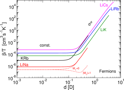
Figure 1: (Color online) Solid lines: Loss rate coefficient $\beta_{L=1}$ divided by $T$ in free 3D space, of the reaction AB + AB $\to$ A₂ + B₂ for different reactive fermionic polar molecules AB = LiNa, KRb, LiK, LiRb, LiCs, as a function of the electric dipole moment. The fermions are considered in a same indistinguishable quantum state. Dashed lines: $\beta_{L=1,M_{L}=0}$ and $\beta_{L=1,|M_{L}|=1}$ components of $L=1$, shown here for AB = LiNa.

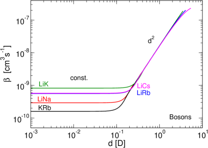
Figure 2: (Color online) Same as Figure 1 for different reactive bosonic polar molecules. The rate coefficient $\beta_{L=0}$ is plotted as a function of the electric dipole moment for $T\to 0$ (Wigner regime). The bosons are considered in a same indistinguishable quantum state.

We report in Fig. 1 and 2 the loss rate coefficient as a function of the induced electric dipole moment $d$, for two indistinguishable fermionic molecules (Fig. 1) and for two indistinguishable bosonic molecules (Fig. 2), for LiNa–LiNa, KRb–KRb, LiK–LiK, LiRb–LiRb and LiCs–LiCs collisions. To converge the results, we use five partial waves, $L=1,3,5,7,9$ for the fermions and $L=0,2,4,6,8$ for the bosons. We used the values of $C_{6}$ and $d_{\text{p}}$ reported in Tab. 1, and the value of $C_{6}=16133$ a.u. of Ref. Kotochigova10 and $d_{p}=0.566$ D of Ref. Ni08 for KRb. We provide a list of the fermionic and bosonic isotopes of each species in Appendix A. These results have been obtained in the regime of ultracold temperature. In this regime, the fermionic rate scales linearly with the temperature (hence we have plotted the rate divided by the temperature) while the bosonic rate is independent of the temperature according to the Bethe-Wigner laws Bethe35 ; Wigner48 . For both cases, the rate scales as a constant in the van der Waals regime where $d\to 0$, and an increasing term in the electric field regime where $d\to d_{\text{p}}$. We note that for large dipole moments, the corresponding dipole length $a_{\text{dd}}=\mu d^{2}/\hbar^{2}$ may exceed the distance between molecules given by the inverse third of the molecular gas density $a_{\text{mm}}=n^{-1/3}$. In such situation, there are no more collisions between molecules. Instead, a dense liquid/solid phase is entered where many-body physics becomes important.

For the fermionic case, in the van der Waals regime, it is seen that the LiNa system is the least reactive, followed by KRb, LiK, LiRb and finally LiCs. Qualitativelly, light masses and small values of $C_{6}$ increase the incident p-wave barrier (this is the case for LiNa) and hence decrease the chance to get high chemical reactivity, while heavy masses and large values of $C_{6}$ decrease the barrier (this is the case for LiCs) and increase the reactivity. In the electric field regime, the same general trend is observed, except now the rate of the KRb system is as high as the LiCs system. Now the rates seem to scale with the reduced mass of the system only. For a given dipole, the electric dipole interaction is the same between the species, only the centrifugal terms differ. Higher mass means smaller barrier so higher loss rate.

For the bosonic case, in the van der Waals regime, KRb are the least reactive molecules, followed by LiNa, LiRb, LiCs and finally LiK. Bosonic particles collide in a s-wave at ultralow energy where no incident barrier is present. Instead, one must invoke the probability for quantum transmission. In the electric field regime, all different systems have the same rate coefficients. This will be explained in the next section.

III.2 Quantum Threshold model

To understand the physical trends seen in the numerical results, we employ an analytical Quantum Threshold model (QT model) Quemener10-QT which provides a universal expression of an ultracold collision (chemical reaction or inelastic collision) with short range unit loss probability. The QT model is a clear and simple model to describe the dependence of an ultracold chemical reaction on the reduced mass and the isotropic van der waals $C_{6}$ coefficient of the molecule-molecule complex, and on the induced dipole moment via the presence of an applied electric field. The QT model assumes that the loss probability scales as

$$P_{L,M_{L}}=p_{{}_{L,|M_{L}|}}\,\bigg{\{}\frac{E_{c}}{E_{*}}\bigg{\}}^{L+1/2}$$ (10)

where $E_{*}$ is a characteristic energy corresponding to the long range interaction of the molecules in a partial wave $L,M_{L}$. $p_{{}_{L,|M_{L}|}}$ is a dimensionless quantity of order of unity, and is estimated by fitting the expression with the numerical results. The thermalized rate coefficient is expressed by

$$\beta_{L,M_{L}}=p_{{}_{L,|M_{L}|}}\,\frac{\hbar^{2}\pi}{\sqrt{2\mu^{3}}}\ \frac{\langle E_{c}^{L}\rangle}{E_{*}^{L+\frac{1}{2}}}\times\Delta$$ (11)

where the brackets denote a Maxwell-Boltzmann distribution over the collision energy to the power $L$. $\Delta=2$ if the particles are in indistinguishable states and $\Delta=1$ if they are in distinguishable states Burke-PHD .

III.2.1 QT model for p-wave collisions

For p-wave collision ($L=1$), we chose the characteristic energy $E_{*}$ equal to the height of the incident barrier, $E_{{}_{L,|M_{L}|}}^{n,m}$, of the effective potential $V_{\text{eff}}$, composed of the strongest attractive potential $-C_{n}/R^{n}$ and the strongest repulsive potential $C_{m}/R^{m}$

$$E_{{}_{L,|M_{L}|}}^{n,m}=\frac{C_{m}\,\left(\frac{n\,C_{n}}{m\,C_{m}}\right)^{\frac{n}{n-m}}-C_{n}\,\left(\frac{n\,C_{n}}{m\,C_{m}}\right)^{\frac{m}{n-m}}}{\left(\frac{n\,C_{n}}{m\,C_{m}}\right)^{\frac{n+m}{n-m}}}.$$ (12)

The position of the barrier is given by

$$R_{{}_{L,|M_{L}|}}^{n,m}=\left(\frac{n\,C_{n}}{m\,C_{m}}\right)^{\frac{1}{n-m}}.$$ (13)

The combinations of $n$ and $m$ are given in Tab. 2 with the corresponding height of the barriers. For the van der Waals regime and for either $|M_{L}|=0,1$, the height of the barrier is made by the the attractive van der Waals interaction $-C_{6}/R^{6}$ and the repulsive centrifugal term $C_{2}/R^{2}\equiv\hbar^{2}\,L(L+1)/(2\mu R^{2})$ with $L=1$, giving rise to a characteristic energy $E_{{1,(0,1)}}^{6,2}$. For the electric field regime and for $|M_{L}|=0$, the height of the barrier is made by the attractive dipole-dipole interaction $-C_{3}(1,1;0)/R^{3}\equiv-[(4/5)\,d^{2}/(4\pi\varepsilon_{0})]/R^{3}$ and the repulsive centrifugal term $C_{2}/R^{2}\equiv\hbar^{2}\,L(L+1)/(2\mu R^{2})$ with $L=1$, giving rise to a characteristic energy $E_{{1,0}}^{3,2}$. Finally, for the electric field regime and for $|M_{L}|=1$, the height of the barrier is made by an attractive $-C_{4}/R^{4}\equiv-[(72\,\mu/(875\,\hbar^{2}))\,d^{4}/(4\pi\varepsilon_{0})^{2}]/R^{4}$ and the repulsive dipole-dipole interaction $-C_{3}(1,1;1)/R^{3}\equiv+[(2/5)\,d^{2}/(4\pi\varepsilon_{0})]/R^{3}$, giving rise to a characteristic energy $E_{{1,1}}^{4,3}$. The $-C_{4}/R^{4}$ attractive interaction comes from the coupling between the $L=1$ and $L=3$ of the $|M_{L}|=1$ component. This is demonstrated in Appendix B.

Table 2: Characteristic energies $E_{*}$ for $L=1,|M_{L}|=0,1$ in the van der Waals (vdW) and electric (elec.) regime.

regime	$|M_{L}|$	- $C_{n}/R^{n}$	$C_{m}/R^{m}$	$E_{{}_{L=1,|M_{L}|}}^{n,m}$
vdW	0,1	- $\frac{C_{6}}{R^{6}}$	$\frac{\hbar^{2}\,L(L+1)}{2\,\mu\,R^{2}}$	$\left(\frac{8\,\hbar^{6}}{54\,\mu^{3}\,C_{6}}\right)^{1/2}$
elec.	0	- $\frac{(4/5)\,d^{2}}{4\pi\varepsilon_{0}\,R^{3}}$	$\frac{\hbar^{2}\,L(L+1)}{2\,\mu\,R^{2}}$	$\frac{25\,\hbar^{6}}{108\,\mu^{3}}\left(\frac{d^{2}}{4\pi\varepsilon_{0}}\right)^{-2}$
elec.	1	- $\frac{72\,\mu\,d^{4}}{875\,\hbar^{2}\,(4\pi\varepsilon_{0})^{2}\,R^{4}}$	$\frac{(2/5)\,d^{2}}{4\pi\varepsilon_{0}\,R^{3}}$	$\frac{(875/24)^{3}\,\hbar^{6}}{10000\,\mu^{3}}\left(\frac{d^{2}}{4\pi\varepsilon_{0}}\right)^{-2}$

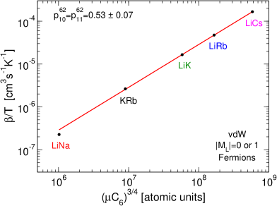
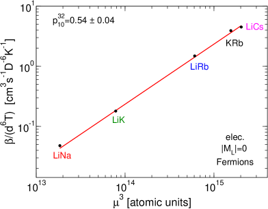
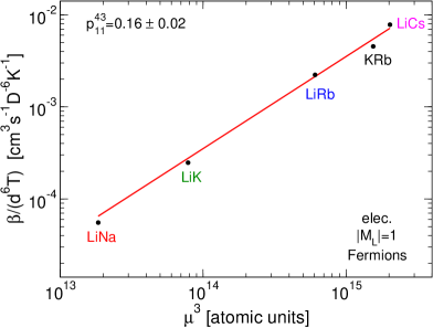
Figure 3: (Color online) Top panel: Van der Waals regime for $M_{L}=0$ and $|M_{L}|=1$. The quantity $\beta_{1,0}^{6,2}=\beta_{1,1}^{6,2}$ divided by $T$ is plotted as a function of $(\mu\,C_{6})^{3/4}$. Middle panel: Electric field regime for $M_{L}=0$. The quantity $\beta_{1,0}^{3,2}$ divided by $d^{6}\,T$ is plotted as a function of $\mu^{3}$. Bottom panel: Electric field regime for $|M_{L}|=1$. The quantity $\beta_{1,1}^{4,3}$ divided $d^{6}\,T$ is plotted as a function of $\mu^{3}$.

Replacing these three values of $E_{*}$ into Eq.(11) for $L=1$ and assuming $\langle E_{c}\rangle=3k_{B}T/2$, where $k_{B}$ is the Boltzmann constant and $T$ the temperature, we arrive at the following expressions for the $|M_{L}|=0,1$ rate as $d\to 0$ in the van der Waals regime

$$\beta_{L=1,|M_{L}|=0,1}^{\text{ vdW}}=\\ p_{1,(0,1)}^{6,2}\ \frac{\pi}{8}\,\left(\frac{3^{13}\,\mu^{3}\,C_{6}^{3}}{\hbar^{10}}\right)^{1/4}\,k_{B}T\times\Delta.$$ (14)

with

$$p_{1,(0,1)}^{6,2}=0.53\pm 0.07.$$ (15)

The $|M_{L}|=0$ rate as $d\to d_{\text{p}}$ in the electric field regime is

$$\beta_{L=1,|M_{L}|=0}^{\text{ elec}}=p_{1,0}^{3,2}\ \frac{3\pi}{8}\,\left(\frac{6^{9}}{5^{6}}\right)^{1/2}\,\frac{\mu^{3}}{\hbar^{7}}\\ \,\frac{d^{6}}{(4\pi\varepsilon_{0})^{3}}\,k_{B}T\times\Delta$$ (16)

with

$$p_{1,0}^{3,2}=0.54\pm 0.04.$$ (17)

Finally, the $|M_{L}|=1$ rate as $d\to d_{\text{p}}$ in the electric field regime is given by

$$\beta_{L=1,|M_{L}|=1}^{\text{ elec}}=p_{1,1}^{4,3}\ \frac{3\pi}{8}\,\left(20000\,(24/875)^{3}\right)^{3/2}\,\frac{\mu^{3}}{\hbar^{7}}\\ \,\frac{d^{6}}{(4\pi\varepsilon_{0})^{3}}\,k_{B}T\times\Delta$$ (18)

with

$$p_{1,1}^{4,3}=0.16\pm 0.02.$$ (19)

The coefficients $p_{L,|M_{L}|}^{n,m}$ associated with the characteristic energies $E_{{}_{L,|M_{L}|}}^{n,m}$, are found by confronting the analytical results in Eq. (14), Eq. (16), and Eq. (18) with our numerical calculations of Fig. 1. The quantity $\beta_{L=1,|M_{L}|=0,1}^{\text{ vdW}}$ divided by $T$ obtained from the numerical results, is plotted as a function of the quantity $(\mu\,C_{6})^{3/4}$ for the van der Waals regime in the top panel of Fig. 3. The quantities $\beta_{L=1,|M_{L}|=0}^{\text{ elec}}$ and $\beta_{L=1,|M_{L}|=1}^{\text{ elec}}$ divided by $d^{6}$ and $T$ are plotted as a function of the quantity $\mu^{3}$ for the electric field regime for the $|M_{L}=0|$ and $|M_{L}=1|$ component in the middle and bottom panels of Fig. 3 respectively, for the different fermionic reactive systems. We find that the numerical results fit a line, confirming the validity of the QT model analysis (the fitting uncertainty of the lines provides an uncertainty to the $p_{L,|M_{L}|}^{n,m}$ parameters). The fitting parameters are the slope of these lines and are reported in Eq. (15), Eq. (17) and Eq. (19).

We see that both components $|M_{L}|=0,1$ analytical rates (Eq.(14)) at ultracold temperature are the same in the van der Waals regime and are dictated by a $d^{6}$ dependence in the electric regime (Eq.(16) and Eq. (18)) with different magnitudes. These expressions provide a clear explanation of the trends observed numerically. The loss rate behaves as $(\mu\,C_{6})^{3/4}$ in the van der Waals regime. In the electric field regime, the loss rate scales as $\mu^{3}$, increasing only with the mass. In both regimes, these expressions explain why fermionic LiNa is the least reactive alkali polar species and fermionic LiCs is the most reactive one.

We note that the results of $p_{1,(0,1)}^{6,2}=0.53\pm 0.07$ is in very good agreement with the analytical expression of $2^{19/4}\,\pi/(3^{17/4}\,[\Gamma(3/4)]^{2})=0.528$ found using a Quantum Defect Theory (QDT) Idziaszek10-PRL . The values $p_{1,0}^{3,2}=0.54\pm 0.04$ and $p_{1,1}^{4,3}=0.16\pm 0.02$ for the $1/R^{3}$ interaction in the electric field regime have not to our knowledge been determined analytically in a QDT framework.

We also note that these constants barely change between the regime dominated by the van der Waals interaction and the regime dominated by an electric field interaction for the $|M_{L}|=0$ component. The ratio of the $|M_{L}|=1$ over the $|M_{L}|=0$ component in the electric field regime is 0.003. As a consequence, the $|M_{L}|=1$ component is negligible in the electric regime, as seen in Fig. 1 for the LiNa system, and one can provide an estimation of the total p-wave rate coefficient for the reactive systems by

$$\beta_{L=1} = \beta_{L=1,|M_{L}|=0}+2\,\beta_{L=1,|M_{L}|=1}$$ (20)

$$\approx 3\,\beta_{L=1,|M_{L}|=0,1}^{\text{ vdW}}+\beta_{L=1,|M_{L}|=0}^{\text{ elec}}$$

$$\approx \frac{\pi}{8}\,\bigg{\{}0.53\times\left(\frac{3^{17}\,\mu^{3}\,C_{6}^{3}}{\hbar^{10}}\right)^{1/4}$$

$$+ 0.54\times\,\left(\frac{2^{9/2}\,3^{11/2}\,\mu^{3}}{5^{3}\,\hbar^{7}}\right)\,\frac{d^{6}}{(4\pi\varepsilon_{0})^{3}}\bigg{\}}\,k_{B}T\times\Delta.$$

III.2.2 QT model for s-wave collisions

For s-wave collisions($L=0,M_{L}=0$), there is no incident barrier because the repulsive centrifugal term vanishes. It is possible however to estimate a characteristic length and energy Gao08 given respectively by

$$a_{n}=\left(\frac{2\,\mu\,C_{n}}{\hbar^{2}}\right)^{\frac{1}{n-2}}\quad;\quad E^{n}_{{}_{L=0,M_{L}=0}}=\frac{\hbar^{2}}{2\,\mu\,a_{n}^{2}}.$$ (21)

In the van der Waals regime, the characteristic energy is $E^{6}_{{0,0}}=\hbar^{3}/\sqrt{2^{3}\,\mu^{3}\,C_{6}}$. In the electric field regime, the electric dipole-dipole interaction vanishes for $L=0$. But as there is a coupling between the $L=0$ and the $L=2$ component in Eq. (8), it is found after diagonalisation, that the electric dipole interaction behaves as a $-C_{4}/R^{4}$ with $C_{4}=4\,\mu\,d^{4}/[15\,\hbar^{2}\,(4\pi\varepsilon_{0})^{2}]$ (see Appendix C). In return, this corresponds to a characteristic energy $E^{4}_{{0,0}}=15\,\hbar^{6}\,(4\pi\varepsilon_{0})^{2}/[16\,\mu^{3}\,d^{4}]$. This is summarized in Tab 3.

Table 3: Characteristic energies $E_{*}$ for $L=0,|M_{L}|=0$ in the van der Waals (vdW) and electric (elec.) regime.

regime	$|M_{L}|$	- $C_{n}/R^{n}$	$E_{{}_{L=0,|M_{L}|}}^{n}$
vdW	0	- $\frac{C_{6}}{R^{6}}$	$\frac{\hbar^{3}}{\sqrt{2^{3}\,\mu^{3}\,C_{6}}}$
elec.	0	- $\frac{4\,\mu\,d^{4}}{15\,\hbar^{2}\,(4\pi\varepsilon_{0})^{2}\,R^{4}}$	$\frac{15\,\hbar^{6}}{16\,\mu^{3}}\left(\frac{d^{2}}{4\pi\varepsilon_{0}}\right)^{-2}$

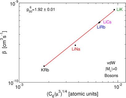
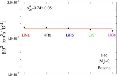
Figure 4: (Color online) Top panel: Van der Waals regime. The quantity $\beta_{0,0}^{6}$ is plotted as a function of $(C_{6}/\mu^{3})^{1/4}$. Bottom panel: Electric field regime. The quantity $\beta_{0,0}^{4}$ divided by $d^{2}$ is plotted for the five different colliding species.

Replacing these two values of $E_{*}$ into Eq.(11) for $L=0$, we arrive at the following expression for the $L=0,|M_{L}|=0$ rate as $d\to 0$ in the van der Waals regime

$$\beta_{L=0,|M_{L}|=0}^{\text{ vdW}}=p_{0,0}^{6}\ \pi\,\left(\frac{2\,\hbar^{2}\,C_{6}}{\mu^{3}}\right)^{1/4}\times\Delta$$ (22)

with

$$p_{0,0}^{6}=1.92\pm 0.01.$$ (23)

The $L=0,|M_{L}|=0$ rate as $d\to d_{\text{p}}$ in the electric field regime is

$$\beta_{L=0,|M_{L}|=0}^{\text{ elec}}=p_{0,0}^{4}\ \pi\,\frac{\sqrt{16/30}}{\hbar}\,\frac{d^{2}}{4\pi\varepsilon_{0}}\times\Delta$$ (24)

with

$$p_{0,0}^{4}=3.74\pm 0.05.$$ (25)

Compared to $L=1$, the rates at ultracold temperature for $L=0$ behave now as $(C_{6}/\mu^{3})^{1/4}$ in the van der Waals regime, making bosonic KRb molecules the least reactive ones and bosonic LiK molecules the most reactive ones, due to the interplay between the $C_{6}$ coefficients and the cube of the mass. In the electric field regime, the rates behave as $d^{2}$ and are independent of the mass, so that for the same induced dipole, all bosonic polar molecules react with the same rate coefficient. The coefficients $p_{L,|M_{L}|}^{n}$ associated with the characteristic energies $E_{{}_{L,|M_{L}|}}^{n}$, are found by plotting the quantity $\beta_{L=0,|M_{L}|=0}^{\text{ vdW}}$ obtained from the numerical results of Fig. 2 as a function of the quantity $(C_{6}/\mu^{3})^{1/4}$ for the van der Waals regime in the top panel of Fig. 4, and the quantity $\beta_{L=0,|M_{L}|=0}^{\text{ elec}}$ divided by $d^{2}$ for the electric regime in the bottom panel of Fig. 4, for the different bosonic reactive systems. As for the fermionic case, the numerical results form a line for the first plot and are constant for the second plot, validating the QT model analysis. Again, we note that the results of $p_{0,0}^{6}=1.92\pm 0.01$ in Eq. (23) is in very good agreement with the analytical expression of $8\,\pi/[\Gamma(1/4)]^{2}=1.912$ found using a Quantum Defect Theory Idziaszek10-PRL or a Quantum Langevin Theory (QL) Gao10 . The value of $p_{0,0}^{4}=3.74\pm 0.05$ agrees within 7% with the analytical expression of 4 from a Quantum Langevin Theory Gao11 using the $-C_{4}/R^{4}$ interaction in the electric field regime. One can formulate a good approximation for the s-wave loss rate coefficients by

$$\beta_{L=0} = \beta_{L=0,|M_{L}|=0}^{\text{ vdW}}+\beta_{L=0,|M_{L}|=0}^{\text{ elec}}$$ (26)

$$\approx \pi\,\bigg{\{}1.92\times\left(\frac{2\,\hbar^{2}\,C_{6}}{\mu^{3}}\right)^{1/4}$$

$$+ 3.74\times\frac{\sqrt{16/30}}{\hbar}\,\frac{d^{2}}{4\pi\varepsilon_{0}}\bigg{\}}\times\Delta.$$

The formulas from Eq. (14) to Eq. (19) and from Eq. (22) to Eq. (25) can be used to determine the inelastic and reactive collisional properties of other atom-atom, atom-molecule or molecule-molecule collisions, provided that full loss occurs when they encounter one another. This case can occur for molecules of category 2 (NaK, NaRb, NaCs, KCs, RbCs) if the molecules are not in their absolute ground state, for example in a higher vibrational state, where inelastic molecule-molecule collision can occur or when the reactants have higher energy than the products so that an exoergic reaction can take place. What is left unknown is the $C_{6}$ coefficients (except for RbCs), for each of these initial ro-vibrational states of these molecules and has to be calculated individually. For the RbCs molecule the $C_{6}$ coefficients have been calculated as a function of vibrational quantum number in Ref. Kotochigova10 .

We provide in Appendix D the corresponding QT expressions for the imaginary part of the scattering lengths for s-wave collisions and scattering volumes for p-wave collisions.

IV Dynamics in two-dimensional space

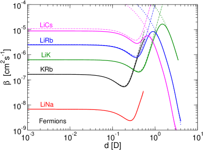
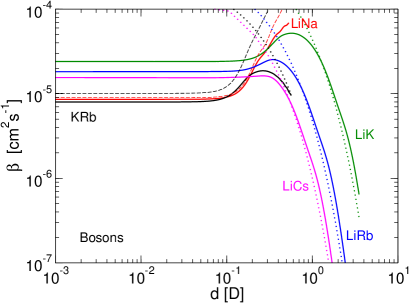
Figure 5: (Color online) Loss rate coefficients for different reactive polar molecules in confined 2D space, for indistinguishable fermions (top panel) and indistinguishable bosons (bottom panel). The frequency of the 1D trap is $\nu=20$ kHz and the temperature is $T=500$ nK. The dashed lines represent a model based on the rescaled 3D rate coefficients for $a_{\text{dd}}\ll a_{\text{ho}}$, and the dotted lines represent a model based on a functional form (Ref. Julienne11-PCCP for example) for $a_{\text{dd}}\gg a_{\text{ho}}$.

For the confined 2D scattering we use the same formalism developed in Ref. Quemener10-2D ; Quemener11-FULL . The confinement is given by an optical lattice in the $\hat{z}$ direction, which we approximate by a harmonic oscillator potential $V_{\text{ho}}=\mu\omega^{2}z^{2}/2$ of frequency $\nu$ and angular frequency $\omega=2\,\pi\,\nu$. One can also define a harmonic oscillator confinement length $a_{\text{ho}}=\sqrt{\hbar/(\mu\,\omega)}$. We consider the dynamics of two molecules in the ground state of this harmonic oscillator. In confined space, $M_{L}$ remains a good quantum number. Additional selection rules apply and for indistinguishable bosons, $|M_{L}|=0$, while for indistinguishable fermions, $|M_{L}|=1$ Quemener10-2D ; Quemener11-FULL , for molecules in the ground state of the harmonic confinement. We present in Fig. 5 the loss rate coefficient for a confinement of $\nu=20$ kHz as a function of the dipole moment for a given temperature $T=500$ nK, for the fermionic species (top panel) and the bosonic species (bottom panel). We use fourty partial waves, $L=1-79$ for the fermions and $L=0-78$ for the bosons, to converge the results. At small electric dipoles, when $a_{\text{dd}}\ll a_{\text{ho}}$, the collisions are quasi-2D (q2D) and the loss rate coefficients display a similar behavior than their 3D counterpart for $|M_{L}|=1$ for the indistinguishable fermions and for $|M_{L}|=0$ for the indistinguishable bosons. At large electric dipoles and for LiK, LiRb, LiCs, when $a_{\text{dd}}\gg a_{\text{ho}}$, the collisions are fully 2D and the loss rate coefficients show a suppression as discussed in Ref. Ticknor10 ; Quemener10-2D ; Micheli10-PRL ; Idziaszek10-RAPID ; Quemener11-FULL ; Dincao10 ; Julienne11-PCCP .

For the quasi-2D regime $a_{\text{dd}}\ll a_{\text{ho}}$, we compare in dashed lines in Fig. 5 a two dimensional loss rate coefficient rescaled from the numerical calculation in three dimensions Petrov01 ; Li09 ; Micheli10-PRL from the previous section for $L=1$

$$\beta^{q2D}=\frac{3}{2}\,\frac{\beta^{3D}}{\sqrt{\pi}\,a_{\text{ho}}}=\frac{3}{2}\,\sqrt{\frac{\mu\,\omega}{\pi\,\hbar}}\,\beta^{3D}$$ (27)

where the factor 3/2 accounts for the difference of the mean energies in 3D and 2D for a given temperature $T$ (in 3D, $\langle E_{c}\rangle=3k_{B}T/2$ while in 2D, $\langle E_{c}\rangle=k_{B}T$). For $L=0$, we get

$$\beta^{q2D}=\frac{\beta^{3D}}{\sqrt{\pi}\,a_{\text{ho}}}=\sqrt{\frac{\mu\,\omega}{\pi\,\hbar}}\,\beta^{3D}.$$ (28)

We found for the fermions a good agreement between the numerical 2D rates (in solid lines) and the rescaled from 3D rates (dashed lines). For the bosons, a good agreement is found for the LiNa system, but not for the other systems like KRb for example, even if the order of magnitude is right. For bosons, threshold laws display a logarithmic dependence and are not accounted in Eq. (28). The QT formulas which describe the numerical 3D rates can also be rescaled in the same manner so that a good approximation to the loss rate coefficient for fermions in the quasi-2D regime $a_{\text{dd}}\ll a_{\text{ho}}$ is given by

$$\beta^{q2D}_{L=1} = 2\times\frac{3}{2}\,\sqrt{\frac{\mu\,\omega}{\pi\,\hbar}}\,\beta^{3D}_{|M_{L}|=1}$$ (29)

$$\approx 3\sqrt{\frac{\mu\,\omega}{\pi\,\hbar}}\,\bigg{\{}0.53\times\left(\frac{3^{13}\,\mu^{3}\,C_{6}^{3}}{\hbar^{10}}\right)^{1/4}$$

$$+ 0.16\times\frac{3\pi}{8}\,\left(\frac{20000}{27}\frac{72}{875}\right)^{3/2}\,\frac{\mu^{3}}{\hbar^{7}}$$

$$\frac{d^{6}}{(4\pi\varepsilon_{0})^{3}}\bigg{\}}\,k_{B}T\times\Delta.$$

For bosons, the rescaled QT formula is

$$\beta^{q2D}_{L=0} = \sqrt{\frac{\mu\,\omega}{\pi\,\hbar}}\,\beta^{3D}_{|M_{L}|=0}$$ (30)

$$\approx \sqrt{\frac{\pi\,\mu\,\omega}{\hbar}}\,\bigg{\{}1.92\times\left(\frac{2\,\hbar^{2}\,C_{6}}{\mu^{3}}\right)^{1/4}$$

$$+ 3.74\times\frac{\sqrt{16/30}}{\hbar}\,\frac{d^{2}}{4\pi\varepsilon_{0}}\bigg{\}}\times\Delta$$

but is only a good approximation for LiNa.

For the 2D regime $a_{\text{dd}}\gg a_{\text{ho}}$, we compare in Fig. 5 a functional form provided in Refs. Julienne11-PCCP ; Buchler07 ; Micheli07 ; Micheli10-PRL ; Ticknor09 ; Ticknor10 ; Dincao10 . We found that the forms

$$\beta^{2D}=2\times 13\,\frac{\hbar}{\mu}\left(\frac{E_{c}}{\hbar\,\omega/2}\right)^{2}\,e^{-2\,(a_{\text{dd}}/a_{\text{ho}})^{2/5}}\times\Delta$$ (31)

for indistinguishable fermions, and

$$\beta^{2D}=13\,\frac{\hbar}{\mu}\left(\frac{E_{c}}{\hbar\,\omega/2}\right)^{2}\,e^{-2\,(a_{\text{dd}}/a_{\text{ho}})^{2/5}}\times\Delta$$ (32)

for indistinguishable bosons fit well the numerical data. These formulas are reported in dotted lines in Fig. 5. We find a coefficient of $13$ in front of the exponential and a coefficient of $2$ inside the exponential, by fitting our numerical results. These values are different from the values found in Ref. Julienne11-PCCP . This is attributed to the different regimes of collision energies and confinements involved in the fitting. It has been shown in Ref. Julienne11-PCCP that the fitting parameters of the functional form may differ for different values of the collision energies.

V Conclusion

By computing the $C_{6}$ coefficients for different pairs of alkali polar molecules of LiNa, LiK, LiRb, and LiCs, and using an available one for KRb, we estimated the quenching rate coefficient assuming full loss when they encounter one another, for the fermionic species and for the bosonic species, both for the van der Waals regime and the electric field regime. We found that, at ultracold temperature, fermionic LiNa is the least reactive system while LiCs is the most in the van der Waals regime and electric field regime, due mainly to the increase of the $C_{6}$ coefficient for the former regime and due to the increase of the mass for the later. Bosonic KRb molecules are found to be the least reactive ones while LiK the most in the van der Waals regime. All the bosonic molecules were found to have the same universal reactive rate in the electric field regime. These behaviors were all explained using a Quantum Threshold model. From our numerical results, we found analytical expressions for the reactive rate coefficients for fermionic and bosonic molecules, in the van der Waals and electric field regime. These expressions can be used for other type of systems, such as atom-molecule or molecule-molecule collisions assuming full inelastic or reactive loss, if the corresponding $C_{6}$ coefficients are known. For example, the analytical expressions can be applied to collision of non-ground state molecules of NaK, NaRb, NaCs, KCs and RbCs. The present study provides useful information about collisional properties of heteronuclear alkali polar molecules for which increasingly experimental interest is devoted. Future studies will consider the vibrational and rotational dependence of the $C_{6}$ coefficient of the heteronuclear alkali molecules, the higher anisotropic terms in the long-range interaction, as well as the effect of higher collision energies, when more partial waves dominate.

Appendix A: Characteristics of the heteronuclear alkali molecules

We provide in Table 4 a summary of the characteristics of the fermionic and bosonic isotopes studied in this work. Conversion factors from atomic units (a.u.) to S.I. units are: 1 a.u. of mass is equal to 1822.89 a.m.u. (atomic mass unit), 1 a.u. of electric dipole moment is equal to 2.5417 D, 1 a.u. of $C_{6}$ is equal to 1 E${}_{\text{h}}$a${}^{6}_{0}$ with 1 E${}_{\text{h}}$ (Hartree) equal to 4.35974394$\times$10^-18 J and 1 a₀ (Bohr radius) equal to 0.529177$\times$10^-10 m.

Table 4: Fermionic (F) or bosonic (B) character, isotope, reduced molecule-molecule mass $\mu$ (in a.u.), $C_{6}$ coefficient (in a.u.) and permanent electric dipole moment $d_{\text{p}}$ (in D) for the different heteronuclear alkali molecules.

F/B	isotope	$\mu$ (a.u.)	$C_{6}$ (a.u.)	$d_{\text{p}}$ (D)
F	6Li23Na	26436	3880	0.531
B	7Li23Na	27349
F	40K87Rb	115638	16133	0.566
B	41K87Rb	116547
F	7Li40K	42820	524000	3.513
B	6Li40K	41907
F	6Li87Rb	84695	1070000	4.046
B	7Li87Rb	85608
F	6Li133Cs	126618	3840000	5.355
B	7Li133Cs	127531

Appendix B: Height of the adiabatic barrier for the $|M_{L}|=1$ component in electric field. Mixing $L=1$ and $L=3$.

In this case, we have two diabatic effective potential curves

$$V_{L=1}(R)=\frac{2\,\hbar^{2}}{2\mu R^{2}}-\frac{C_{6}}{R^{6}}+\frac{(2/5)\,d^{2}}{4\pi\varepsilon_{0}\,R^{3}}$$

$$V_{L=3}(R)=\frac{12\,\hbar^{2}}{2\mu R^{2}}-\frac{C_{6}}{R^{6}}-\frac{(2/5)\,d^{2}}{4\pi\varepsilon_{0}\,R^{3}}$$

and a coupling

$$W(R)=\frac{(2\sqrt{126}/35)\,d^{2}}{4\pi\varepsilon_{0}\,R^{3}}.$$ (34)

In the case of $|W|\ll|V_{L=3}-V_{L=1}|$, the adiabatic effective potential curves are given after diagonalisation by

$$E_{\pm}(R)=V_{L=3/1}(R)\pm\frac{72\,\mu\,d^{4}}{875\,\hbar^{2}\,(4\pi\varepsilon_{0})^{2}\,R^{4}}$$ (35)

and especially the lower one

$$E_{-}(R)=\frac{2\,\hbar^{2}}{2\mu R^{2}}-\frac{C_{6}}{R^{6}}+\frac{(2/5)\,d^{2}}{4\pi\varepsilon_{0}\,R^{3}}-\frac{C_{4}}{R^{4}}$$ (36)

with

$$C_{4}=\frac{72\,\mu\,d^{4}}{875\,\hbar^{2}\,(4\pi\varepsilon_{0})^{2}}.$$ (37)

At large $d$, the most repulsive potential in Eq. (36) is $[(2/5)\,d^{2}]/[4\pi\varepsilon_{0}\,R^{3}]$ and the most attractive is $-C_{4}/R^{4}$ so that the height of the barrier is

$$E_{{}_{L=1,|M_{L}|=1}}^{n=4,m=3}=\frac{(875/24)^{3}\,\hbar^{6}}{10000\,\mu^{3}}\left(\frac{d^{2}}{4\pi\varepsilon_{0}}\right)^{-2}.$$ (38)

Appendix C: Adiabatic potential for the $|M_{L}|=0$ component in electric field. Mixing $L=0$ and $L=2$.

Now we have the two diabatic effective potential curves

$$V_{L=0}(R) = -\frac{C_{6}}{R^{6}}$$

$$V_{L=2}(R) = \frac{6\,\hbar^{2}}{2\mu R^{2}}-\frac{C_{6}}{R^{6}}-\frac{(4/7)\,d^{2}}{4\pi\varepsilon_{0}\,R^{3}}$$

and the coupling between them

$$W(R)=-\frac{2\,d^{2}}{\sqrt{5}\,4\pi\varepsilon_{0}\,R^{3}}.$$ (40)

In the case of $|W|\ll|V_{L=2}-V_{L=0}|$, the adiabatic effective potential curves are given after diagonalisation by

$$E_{\pm}(R)=V_{L=2/0}(R)\pm\frac{4\,\mu\,d^{4}}{15\,\hbar^{2}\,(4\pi\varepsilon_{0})^{2}\,R^{4}}$$ (41)

and especially the lower one

$$E_{-}(R)=-\frac{C_{6}}{R^{6}}-\frac{C_{4}}{R^{4}}$$ (42)

with

$$C_{4}=\frac{4\,\mu\,d^{4}}{15\,\hbar^{2}\,(4\pi\varepsilon_{0})^{2}}.$$ (43)

Appendix D: QT expression for imaginary scattering lengths and scattering volumes

We provide here the analytical QT expressions for imaginary scattering lengths and imaginary scattering volumes. If we define the scattering length and the scattering volume (see Ref. Bala97 ) by

$$a = a_{r}-i\,a_{i}=-\delta(k)/k$$ (44)

$$V = V_{r}-i\,V_{i}=-\delta(k)/k^{3},$$ (45)

for vanishing wave-vectors $k\to 0$, the loss rate can be written as

$$\beta_{L=0} = \bigg{(}4\,\hbar\,\pi\,a_{i}/\mu\bigg{)}\times\Delta$$

$$\beta_{L=1,M_{L}} = \bigg{(}4\,\hbar\,\pi\,k^{2}\,V_{i}/\mu\bigg{)}\times\Delta$$ (46)

for one component $M_{L}$. Similarly, the elastic rate is given by

$$\beta^{\text{el}}_{L=0} = \bigg{(}4\,\hbar\,\pi\,k\,|a|^{2}/\mu\bigg{)}\times\Delta$$

$$\beta^{\text{el}}_{L=1,M_{L}} = \bigg{(}4\,\hbar\,\pi\,k^{5}\,|V|^{2}/\mu\bigg{)}\times\Delta.$$ (47)

To get the corresponding cross sections, one has to divide the rates by the relative velocity $v=\hbar\,k/\mu$. Identifying the loss rate with the QT model, one gets the imaginary scattering length in the van der Waals regime

$$a_{i}=1.92\times\bigg{(}\frac{\mu^{1/4}\,C_{6}^{1/4}}{2^{7/4}\,\hbar^{1/2}}\bigg{)},$$ (48)

the imaginary scattering length in the electric field regime

$$a_{i}=3.74\times\,\bigg{(}\frac{\mu}{\hbar^{2}\,\sqrt{30}}\bigg{)}\,\frac{d^{2}}{4\pi\varepsilon_{0}}$$ (49)

the imaginary scattering volume in the van der Waals regime

$$V_{i}=0.53\times\bigg{(}\frac{3^{9/4}\,\mu^{3/4}\,C_{6}^{3/4}}{32\,\hbar^{3/2}}\bigg{)},$$ (50)

and the imaginary scattering volume in the electric field regime

$$V_{i}=0.54\times\bigg{(}\frac{3^{9/2}\,\mu^{3}}{\hbar^{6}\,2^{1/2}\,5^{3}}\bigg{)}\,\frac{d^{6}}{(4\pi\varepsilon_{0})^{3}}.$$ (51)

In the case of lossy collisions, the imaginary parts $a_{i}$ or $V_{i}$ contributes to the elastic part of the rates. As a consequence, they provide a minimum value for the elastic rates $\beta^{\text{el}}_{L=0}=(4\,\hbar\,\pi\,k\,a_{i}^{2}/\mu)\times\Delta$ for s-wave collisions and $\beta^{\text{el}}_{L=1,M_{L}}=(4\,\hbar\,\pi\,k^{5}\,V_{i}^{2}/\mu)\times\Delta$ for p-wave collisions. In other words, lossy collisions imply non-zero elastic cross sections or rate coefficients.

References

- (1) J. M. Sage, S. Sainis, T. Bergeman, and D. DeMille, Phys. Rev. Lett. 94, 203001 (2005).
- (2) E. R. Hudson, N. B. Gilfoy, S. Kotochigova, J. M. Sage, and D. DeMille, Phys. Rev. Lett. 100, 203201 (2008).
- (3) K.-K. Ni, S. Ospelkaus, M. H. G. de Miranda, A. Pe’er, B. Neyenhuis, J. J. Zirbel, S. Kotochigova, P. S. Julienne, D. S. Jin, and J. Ye, Science 322, 231 (2008).
- (4) J. Deiglmayr, A. Grochola, M. Repp, K. Mörtlbauer, C. Glück, J. Lange, O. Dulieu, R. Wester, and M. Weidemüller, Phys. Rev. Lett. 101, 133004 (2008).
- (5) K. Aikawa, D. Akamatsu, M. Hayashi, K. Oasa, J. Kobayashi, P. Naidon, T. Kishimoto, M. Ueda, and S. Inouye, Phys. Rev. Lett. 105, 203001 (2010).
- (6) S. Ospelkaus, K.-K. Ni, G. Quéméner, B. Neyenhuis, D. Wang, M. H. G. de Miranda, J. L. Bohn, J. Ye, and D. S. Jin, Phys. Rev. Lett. 104, 030402 (2010).
- (7) K.-K. Ni, S. Ospelkaus, D. Wang, G. Quéméner, B. Neyenhuis, M. H. G. de Miranda, J. L. Bohn, J. Ye, and D. S. Jin, Nature, 464 1324 (2010).
- (8) M. H. G. de Miranda, A. Chotia, B. Neyenhuis, D. Wang, G. Quéméner, S. Ospelkaus, J. L. Bohn, J. Ye, and D. S. Jin, Nature Physics, 7, 502 (2011).
- (9) M. Aymar and O. Dulieu, J. Chem. Phys. 122, 204302 (2005).
- (10) J. Deiglmayr, M. Aymar, R. Wester, M. Weidemüller, and Olivier Dulieu, J. Chem. Phys. 129, 064309 (2008).
- (11) P. S. uchowski and J. M. Hutson, Phys. Rev. A 81, 060703(R) (2010).
- (12) J. N. Byrd, J. A. Montgomery Jr., and R. Côté, Phys. Rev. A 82, 010502(R) (2010).
- (13) E. R. Meyer and J. L. Bohn, Phys. Rev. A 82, 042707 (2010).
- (14) E. R. Meyer and J. L. Bohn, Phys. Rev. A 83, 032714 (2011).
- (15) S. Ospelkaus, K.-K. Ni, D. Wang, M. H. G. de Miranda, B. Neyenhuis, G. Quéméner, P. S. Julienne, J. L. Bohn, D. S. Jin, and J. Ye, Science 327, 853 (2010).
- (16) G. Quéméner and J. L. Bohn, Phys. Rev. A 81, 022702 (2010).
- (17) C. Ticknor and S. T. Rittenhouse, Phys. Rev. Lett. 105, 013201 (2010).
- (18) Y. Wang, J. P. D’Incao, C. H. Greene, Phys. Rev. Lett. 106, 233201 (2011).
- (19) Y. Wang, J. P. D’Incao, C. H. Greene, e-print arXiv:1106.6133.
- (20) L. D. Carr, D. DeMille, R. V. Krems, and J. Ye, New J. Phys. 11, 055049 (2009).
- (21) A. Micheli, G. K. Brennen and P. Zoller, Nat. Phys. 2, 341 (2006).
- (22) G. Pupillo, A. Micheli, H.-P. Büchler, and P. Zoller, in Cold Molecules: Theory, Experiment, Applications, edited by R. V. Krems, W. C. Stwalley, and B. Friedrich (CRC Press, Boca Raton, FL, 2009).
- (23) D. DeMille, Phys. Rev. Lett. 88, 067901 (2002).
- (24) S. F. Yelin, K. Kirby, and R. Côté, Phys. Rev. A 74, 050301(R) (2006).
- (25) A. V. Gorshkov, S. R. Manmana, G. Chen, J. Ye, E. Demler, M. D. Lukin, A.-M. Rey, e-print arXiv:1106.1644.
- (26) A. V. Gorshkov, S. R. Manmana, G. Chen, E. Demler, M. D. Lukin, A.-M. Rey, e-print arXiv:1106.1655.
- (27) S. Ospelkaus, A. Pe’er, K.-K. Ni, J. J. Zirbel, B. Neyenhuis, S. Kotochigova, P. S. Julienne, J. Ye and D. S.Jin, Nature Physics 4, 622 (2008).
- (28) S. Kotochigova, E. Tiesinga, and P. S. Julienne, New J. Phys. 11, 055043 (2009).
- (29) Z. Idziaszek and P. S. Julienne, Phys. Rev. Lett. 104, 113202 (2010).
- (30) C. Ticknor, Phys. Rev. A 81, 042708 (2010).
- (31) S. Kotochigova, New J. Phys. 12, 073041 (2010).
- (32) G. Quéméner and J. L. Bohn, Phys. Rev. A 81, 060701(R) (2010).
- (33) A. Micheli, Z. Idziaszek, G. Pupillo, M. A. Baranov, P. Zoller, and P. S. Julienne Phys. Rev. Lett. 105, 073202 (2010).
- (34) Z. Idziaszek, G. Quéméner, J. L. Bohn, and P. S. Julienne Phys. Rev. A 82, 020703(R) (2010)
- (35) B. Gao, Phys. Rev. Lett. 105, 263203 (2010).
- (36) G. Quéméner and J. L. Bohn, Phys. Rev. A 83, 012705 (2011).
- (37) J. P. D’Incao and C. H. Greene, Phys. Rev. A 83, 030702 (2011).
- (38) P. S. Julienne, T. M. Hanna, Z. Idziaszek, Phys. Chem. Chem. Phys., 2011, Advance Article DOI: 10.1039/C1CP21270B, e-print arXiv:1106.0494.
- (39) C. Haimberger, J. Kleinert, P. Zabawa, A. Wakim, and N. P. Bigelow, New. J. Phys. 11, 055042 (2009).
- (40) P. Zabawa, A. Wakim, A. Neukirch, C. Haimberger, N. P. Bigelow, A. V. Stolyarov, E. A. Pazyuk, M. Tamanis, and R. Ferber, Phys. Rev. A 82, 040501(R) (2010).
- (41) A. D. Lercher, T. Takekoshi, M. Debatin, B. Schuster, R. Rameshan, F. Ferlaino, R. Grimm, and H.-C. Nägerl, Eur. Phys. J. D, 2011, Advance article DOI: 10.1140/epjd/e2011-20015-6, e-print arXiv:1101.1409.
- (42) M. Debatin, T. Takekoshi, R. Rameshan, L. Reichsöllner, F. Ferlaino, R. Grimm, R. Vexiau, N. Bouloufa, O. Dulieu, and H.-C. Nägerl, e-print arXiv:1106.0129.
- (43) H.W. Cho, D.J. McCarron, D. L. Jenkin, M. P. Köppinger, and S. L. Cornish, Eur. Phys. J. D, 2011, Advance article DOI: 10.1140/epjd/e2011-10716-1, e-print arXiv:1107.5567.
- (44) J. Deiglmayr, M. Repp, A. Grochola, O. Dulieu, R. Wester, and M. Weidemüller, J. Phys.: Conf. Ser. 264 012214 (2011).
- (45) J. Deiglmayr, M. Repp, O. Dulieu, R. Wester, and M. Weidemüller, e-print arXiv:1107.1060.
- (46) A. Ridinger, S. Chaudhuri, T. Salez, D. R. Fernandes, N. Bouloufa, O. Dulieu, C. Salomon, and F. Chevy, e-print arXiv:1106.0494.
- (47) A. J. Stone, The theory of intermolecular forces, (Clarendon Press, London, 1996).
- (48) K. T. Tang, Phys. Rev. 177, 108 (1969).
- (49) R. Barnett, D. Petrov, M. Lukin, and E. Demler, Phys. Rev. Lett. 96, 190401 (2006).
- (50) G. Herzberg, Spectra of diatomic molecules, 2nd edition (van Nostrand Company, Princeton, 1950).
- (51) J. D. Watts, J. Gauss. and R. J. Bartlett, J. Chem. Phys. 98, 8718 (1993).
- (52) T.H. Dunning, Jr. J., Chem. Phys. 90, 1007 (1989).
- (53) B. P. Prascher, D. E. Woon, K. A. Peterson, T. H., Jr. Dunning, and A. K. Wilson, Theor. Chem. Acct. 128, 69 (2011)
- (54) Kirk Peterson, private communication.
- (55) I. Lim, P. Schwerdtfeger, B. Metz, and H. Stoll, J. Chem. Phys. 122, 104103 (2005).
- (56) H. A. Bethe, Phys. Rev. 47, 747 (1935).
- (57) E. P. Wigner, Phys. Rev. 73, 1002 (1948).
- (58) J. P. Burke Jr., Ph.D. thesis, University of Colorado (1999), available online at http://jilawww.colorado.edu/pubs/thesis/burke.
- (59) B. Gao, Phys. Rev. A 78, 012702 (2008).
- (60) B. Gao, Phys. Rev. A 83, 062712 (2011).
- (61) D. S. Petrov and G. V. Shlyapnikov, Phys. Rev. A 64, 012706 (2001).
- (62) Z. Li and R. V. Krems, Phys. Rev. A 79, 050701(R) (2009).
- (63) H. P. Büchler, E. Demler, M. Lukin, A. Micheli, N. Prokofiev, G. Pupillo, and P. Zoller, Phys. Rev. Lett. 98, 060404 (2007).
- (64) A. Micheli, G. Pupillo, H. P. Büchler, and P. Zoller, Phys. Rev. A 76, 043604 (2007).
- (65) C. Ticknor, Phys. Rev. A 80, 052702 (2009).
- (66) N. Balakrishnan, V. Kharchenko, R. C. Forrey, and A. Dalgarno, Chem. Phys. Lett 280, 5 (1997).