Are Percolation Transitions always Sharpened by Making Networks Interdependent?

Abstract

We study a model for coupled networks introduced recently by Buldyrev et al., Nature 464, 1025 (2010), where each node has to be connected to others via two types of links to be viable. Removing a critical fraction of nodes leads to a percolation transition that has been claimed to be more abrupt than that for uncoupled networks. Indeed, it was found to be discontinuous in all cases studied. Using an efficient new algorithm we verify that the transition is discontinuous for coupled Erdös-Rényi networks, but find it to be continuous for fully interdependent diluted lattices. In 2 and 3 dimension, the order parameter exponent $\beta$ is larger than in ordinary percolation, showing that the transition is less sharp, i.e. further from discontinuity, than for isolated networks. Possible consequences for spatially embedded networks are discussed.

While the theoretical study of single networks has exploded during the last years, relatively little work has been devoted to the study of interdependent networks. This is in stark contrast to the abundance of coupled networks in nature and technology – one might e.g. think of people connected by telephone calls, by roads, by their work relationships, etc. For single networks it is well known that removing nodes can lead to cascades where other nodes become dysfunctional too Motter , and deleting a sufficient fraction of nodes leads to the disappearance of the giant connected cluster. If the network is already close to the transition point, deleting a single node can lead to an infinite cascade similar to the outbreak of a large epidemic in a population.

Assume now that all nodes have to be connected via different types of links in order to remain functional. It was argued in Buldy that in such cases the cascades of failure triggered by removing single nodes should be greatly enhanced, and that the transition between existence and non-existence of a giant cluster of functional nodes should become discontinuous. This claim was backed by a mean field theory that becomes exact for locally tree-like networks (e.g. large sparse Erdös-Rényi (ER) networks), and by numerical simulations for various types of network topologies. In the present paper we show that this view is not entirely correct: For fully interdependent diluted $d$-dimensional lattices, the transition is not only continuous, but it is less sudden than the ordinary percolation (OP) transition for isolated lattices and represents a new universality class.

The problem is best illustrated by an actual case discussed in Buldy , which concerns an electric power blackout in Italy in September 2003 Rosato . According to Buldy (see also Parshani ; Havlin ), the event was possibly triggered by the failure of a single node $i_{0}$ in the electricity network. Nodes in a power networks are in general also linked by a telecommunication network (TN) and need to receive information about the status of the other nodes. In the present case, presumably some nodes in the TN failed, because they were not supplied with power. This then led to the failure of more power stations because they did not receive the necessary information from $i_{0}$, of more TN nodes because they were not supplied with electric power, etc. The ensuing cascade finally affected the entire power grid.

The crucial point here is that each node has to be connected to two distinct networks that provide different services, in order to be viable. At the same time nodes act as bridges to bring supply to other nodes. If a node gets disconnected from one network, it no longer can function and looses also its ability to serve as a connector in the other. The claim in Buldy , to be scrutinized here, is that these cascades of failure are much more abrupt in interdependent networks than in isolated ones, leading to much sharper transitions.

In a single network, the existence of an “infinite” cluster of nodes, making possible the outbreak of a large epidemic, is described by OP. Whether such a large outbreak can happen depends on the average connectivity of the network, characterized by some parameter $p$. If $p$ is below a critical value $p_{c}$, no infinite epidemic can occur, while it occurs with probability $P>0$ if $p>p_{c}$. For $p$ slightly above $p_{c}$, both $P$ and the relative size of the epidemic in a large but finite population scale $\sim(p-p_{c})^{\beta}$, where the order parameter exponent $\beta$ depends on the topology of the network. For ER networks $\beta=1$, while for randomly diluted $d$-dimensional lattices $\beta$ depends on $d$, with $\beta(d=2)=5/36\approx 0.1389$ Stauffer and $\beta(d=3)=0.4170(3)$ Deng . In all these cases $\beta>0$, meaning that the transition is continuous. A discontinuous transition, as found in Buldy ; Havlin , would correspond to $\beta=0$.

Discontinuous percolation transitions have recently been claimed to exist in several other models Achliopt ; Herrmann-Manna-Chen , including explosive percolation Achliopt . The numerical evidence for discontinuity given in Achliopt was supported in numerous papers. It became clear only recently that the transition is actually continuous, although with small $\beta$ and with unusual finite size behavior Costa-Grass-Riordan-Lee . In view of the difficulty to distinguish numerically between a truly discontinuous transition and a continuous one with very small $\beta$, we decided to perform more precise simulations.

The algorithm used in Buldy follows in detail the cascades triggered by removing nodes and, as a result, does not allow one to study large networks with high statistics. In our simulations, instead of removing nodes, we add nodes one by one. Using a modification of the fast Newman-Ziff algorithm Newman , this gives a code which no longer follows entire cascades, as they are broken up into short sub-cascades, and gluing them together would make the algorithm slow again. But it allowed us to obtain high statistics for reasonably large systems.

The model is formally defined as follows: Start with a single set $\cal N$ of $N$ nodes and with two networks $\cal A$ and $\cal B$ that are obtained by linking these nodes (notice that $\cal A$ and $\cal B$ need not be connected, and indeed some nodes in $\cal N$ may be not connected at all, in which case $\cal A$ and $\cal B$ make use only of subsets of $\cal N$; also we do not demand that all links in $\cal A$ and $\cal B$ are different). Typically, we construct $\cal A$ and $\cal B$ by starting with a dense network and deleting randomly links from it, keeping links only with probability $q<1$. In this way, ER networks are constructed by starting with a complete graph and keeping only $L=qN(N-1)/2$ links. Alternatively, diluted regular $d$-dimensional lattices are obtained by starting with a (hyper-)cubic lattice with $N=L^{d}$ nodes and helical boundary conditions, and keeping only a fraction $q$ of the $dN$ links.

On these coupled networks (each obtained by bond percolation with parameter $q$), we study a site percolation problem by retaining only a fraction $p$ of all nodes, calling the set of retained nodes ${\cal N}_{p}$. We define $\cal AB$-clusters as subsets of nodes $\in{\cal N}_{p}$ that are connected both in $\cal A$ and in $\cal B$. More precisely, assume that $C=\{i_{1},i_{2},\ldots i_{m}\}$ is a subset of nodes in ${\cal N}_{p}$. We call it a (connected $\cal AB$-) cluster, if any two points $i\in C$ and $j\in C$ are connected by (at least) two paths: one path using only links $\in\cal A$, and nodes only $\in C$, and another path using only links $\in\cal B$, also using nodes only $\in C$. Notice that we do not allow paths that involve nodes outside $C$, i.e. $\cal AB$-clusters are ‘self-sustaining’. The “order parameter” $S=m_{\rm max}/N$ is then the relative size of the largest $\cal AB$-cluster, for given $p$ and $q$.

To find these maximal clusters, we start with an empty initial configuration with no nodes but with a list of all possible links in $\cal A$ and$\cal B$, and set $m_{\rm max}=0$. Then we add nodes one by one. Each time a new node $i$ is added,

(a) We check whether it is linked to any of the existing nodes. If it is not linked to any other node either by $\cal A$ or by $\cal B$ links, we simply insert the next node.

(b) Otherwise, we update the cluster structures in $\cal A$ and $\cal B$ separately by means of the Newman-Ziff algorithm, and denote the sets of nodes linked to $i$ by $C_{\cal A}$ and $C_{\cal B}$. If one of them has size $\leq m_{\rm max}$, then $m_{\rm max}$ cannot increase and we insert the next node.

If not, we check whether the biggest $\cal AB$-cluster in $C_{\cal A}\bigcap C_{\cal B}$ can have a size $>m_{\rm max}$, by following a cascade similar to that in Buldy . If the cascade stops at a cluster size $>m_{\rm max}$, then $m_{\rm max}$ is increased. If it continues to a size $\leq m_{\rm max}$, the cascade is stopped and $m_{\rm max}$ is left unchanged. In either case, we then insert the next node.

(c) This process continues until a preset value $p_{\rm max}$ is reached. Stopping at $p<1$ is crucial for efficiency, as the algorithm slows down dramatically at large $p$. We typically follow the evolution up to $p$ slightly above $p_{c}$ for all realizations, and follow it up to larger values of $p$ for successively fewer runs. This reflects the fact that simulations are slow for $p\gg p_{c}$, but fluctuations are also smaller, so that fewer samples are sufficient.

For ER graphs the model can be simplified, since bond and site dilution both lead again to ER graphs. Hence we do not have to distinguish between them and can skip the site percolation part. The order parameter $S=m_{\rm max}/N$ is then, in the limit $N\to\infty$, a unique function of the average degree $\langle k\rangle$. This function is easily found by arguments analogous to those for single networks.

Consider an isolated ER network with average degree $\langle k\rangle=z$ in the regime where an infinite cluster exists, i.e. where an infection has a non-zero chance to lead to an infinite epidemic. Let $S_{i}$ be the probability that node $i$ gets infected during this epidemic. The probability that $i$ does not get infected is then

$$1-S_{i}=\prod_{<ij>}(1-S^{\prime}_{j}),$$ (1)

where the product runs over all neighbors of $i$. Here, $S^{\prime}_{j}$ is the probability that $j$ is infected, conditioned on it being picked as a node at the end of a link, and we used the fact that the graph is locally tree-like, so all $S^{\prime}_{j}$ are independent. For ER graphs the degree distribution is Poisson, and $S^{\prime}$ and $S$ obey the same statistics. Averaging Eq. (1) over all nodes and topologies gives then bollobas ; newman

$$1-S=\sum_{k}{e^{-z}z^{k}\over k!}(1-S)^{k}=e^{-zS},$$ (2)

where we dropped the index on $S$. Otherwise said, the probability $S$ that any site is linked to the infinite cluster is $1-\exp(-zS)$. For two interdependent ER networks with average degrees $z_{\cal A}$ and $z_{\cal B}$, the chance to belong to the infinite ${\cal AB}$-cluster is equal to the probability to be linked to it both via $\cal A$ and via $\cal B$, giving

$$S=(1-e^{-z_{\cal A}S})(1-e^{-z_{\cal B}S}).$$ (3)

Although this is much simpler than the theory presented in Buldy , it is exactly equivalent. It is generalized trivially to $>2$ interdependent networks Gao , and to other types of interdependencies Son . If $z_{\cal A}=z_{\cal B}=z$, one finds only the solution $S=0$ for $z<z_{c}=2.455407\ldots$, while a second stable solution $S>0$ exists for $z>z_{c}$. Just above threshold, $S_{c}=0.511699\ldots$.

Figure 1: (Color online) Plot for $S=\langle m_{\rm max}\rangle/N$ against $z$, for two interdependent ER networks with degrees $z_{\cal A}=z_{\cal B}=z$. For technical reasons, each curve does not correspond to a fixed value of $N$, but of $N_{0}=4N/z$. The grey curve is the solution of Eq. (3). The intersection of the horizontal and vertical lines indicate the point $(z_{c},S_{c})$.

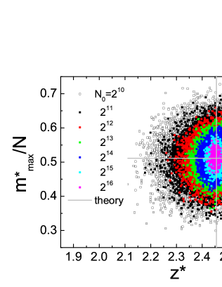
Figure 2: (Color online) Scatter plot for $m_{\rm max}/N$ against $z$, just after the largest jump in $m_{\rm max}$. Color corresponds to a fixed value of $N$. The lines indicate the analytic prediction for the point $(z_{c},S_{c})$, according to Eq. (3).

Results from our numerical simulations for ER graphs, using the algorithm outlined above, are shown in Figs. 1 and 2. Figure 1 shows $S$ versus $z$ for networks of different sizes. Each curve is based on $10^{4}$ runs, except for the largest $N$. The data indeed approach the theoretical curve (indicated in grey), as $N\to\infty$. While Fig. 1 demonstrates that the theory gives the correct $z_{c}$, it is much harder to argue that it gives also the correct $S_{c}$. To see this, we notice that $m_{\rm max}/N$ makes in each run exactly one big jump, from $\approx 0$ to $\approx S_{c}$. The values of $z$ and $S$ just after the jump are shown as scatter plots in Fig. 2. We see clouds of points that are indeed centered near $z_{c}$ and $S_{c}$, and whose sizes decrease with $N$.

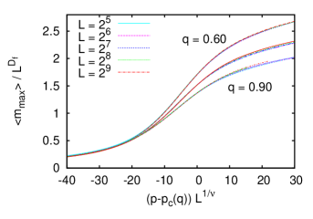
Figure 3: (Color online) Data collapse for $\langle m_{\rm max}\rangle/L^{D_{f}}$ against $(p-p_{c})L^{1/\nu}$, for 2-$d$ lattices. Each set of curves corresponds to one value of $q$, while each curve within each set corresponds to a system size $L$. For this plot, $\nu=1.19$ and $D_{f}=1.85$ were used, and the values of $p_{c}$ are $0.96025,0.77556$, and $0.6544$ for $q=0.6,0.75$, and $0.9$. Due to universality of the scaling function $f(z)$ we can also collapse the three set of curves, by multiplying $m_{\rm max}/L^{D_{f}}$ and $(p-p_{c})L^{1/\nu}$ by suitable $q$-dependent factors (data not shown).

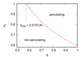
Figure 4: (Color online) Critical values $p_{c}$ versus $q$ for two coupled 2-$d$ lattices. Error bars are much smaller than the symbol sizes. Notice that the bond percolation threshold on the square lattice is $q_{c}=1/2$, thus the curve cannot extend below $q<0.5$. The transition is in the same universality class even for $q=q_{\rm min}=0.5757(4)$, where $p_{c}=1$ and the model simplifies, as no site percolation is involved. For $q\to 1$, the model crosses over to OP.

For bond percolation on the square lattice, the OP threshold is at $q_{c}=1/2$ Stauffer . We therefore look for $\cal AB$-percolation in the parameter range $1/2<q<1$. We assume the usual finite size scaling (FSS) ansatz Stauffer

$$\langle m_{\rm max}\rangle=L^{D_{f}}f[(p-p_{c})L^{1/\nu}]\;,$$ (4)

where $\nu$ is the correlation length exponent, $D_{f}=d-\beta/\nu$ is the fractal dimension of the incipient infinite cluster, and $f(z)$ is a smooth (indeed analytic) function. According to this ansatz, we expect a data collapse if we plot $\langle m_{\rm max}\rangle/L^{D_{f}}$ against $(p-p_{c})L^{1/\nu}$. Three such data collapses are shown in Fig. 3, each for a different value of $q$. Each of the three “curves” in this figure are indeed several collapsed curves corresponding to different values of $L$ in the range $2^{5}$ to $2^{9}$, obtained from more than $10^{6}$ realizations for the smallest lattice and $\approx 10^{4}$ for the largest. For all curves the same values of $D_{f}$ and $\nu$ were used, while $p_{c}$ depends of course on $q$. The values of $p_{c}$ are plotted against $q$ in Fig. 4.

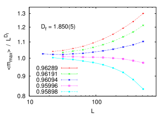
Figure 5: (Color online) Log-log plot of $\langle m_{\rm max}\rangle/L^{D_{f}}$ against $L$, for 2-d interdependent percolation at $q=0.60$ and at fixed values of $p$. At the critical point ($p_{c}=0.96025(20)$) we expect a straight line. The value of the fractal dimension $D_{f}$ is chosen such that this line is horizontal.

Figure 6: (Color online) Log-log plot of $S=\langle m_{\rm max}\rangle/L^{2}$ against $p-p_{c}$, for 2-d interdependent percolation with $q=0.60$. The slight upward curvature for large $p-p_{c}$ indicates the limit of the critical region, while the upward curvature for $p-p_{c}\to 0$ is due to finite size corrections.

The fact that data collapse was obtained in Fig. 3 for $q$-independent values of the exponents indicates that these exponents are universal for $q_{\rm min}\leq q<1$. But a closer inspection of Fig. 3 shows that the quality of the collapse deteriorates as $q\to 1$, due to the expected cross-over to OP (for $q\to 1$, $\cal A$ and $\cal B$ become identical, and the problem crosses over to OP). Thus we use data for $q=0.6$ for more detailed analyses. Figure 5 shows that $m_{\rm max}\sim L^{D_{f}}$ for $p_{c}=0.96025(20)$, with $D_{f}=1.850(5)$, while Fig. 6 shows that $m_{\rm max}\sim(p-p_{c})^{\beta}$ in the limit $L\to\infty$, with $\beta=0.172(2)$ (for a plot with higher resolution see the supplementary material (SM)). Both exponents are clearly different from the values for OP. Indeed, $\beta$ is larger than the value $5/36=0.1389$ for OP, showing that the transition is not more abrupt than in OP, as claimed in Buldy , but less so!

For $d=3$ we also studied systems of up to $2^{18}$ sites, with roughly the same number of realizations as for 2d, and with similar results (see the SM for details): There are also important corrections to scaling, if $q$ is taken too large, but they decrease strongly when $q$ is taken as small as possible. For $q=0.40$ we obtain $p_{c}=0.871(1),\beta=0.51(1),\nu=0.86(1),$ and $D_{f}=2.40(1)$. These values satisfy (like the 2-d exponents) the scaling relation $D_{f}=d-\beta/\nu$, and again they are incompatible with OP (where $\beta=0.4170(3),\nu=0.8734(5),D_{f}=2.5226(1)$ Deng ). As in 2-d, $\beta$ is clearly larger than in OP, indicating that the transition is again less sharp, rather than more abrupt.

In summary, we have shown that coupling two interdependent networks does not generically make the percolation transition more abrupt or discontinuous. Rather, the outcome depends on the network topologies. Real networks (e.g. transportation, telephone, …) often are locally embedded in space, thus their behavior might resemble more that of regular lattices than that of small world networks. The reason why the claim of Buldy does not hold universally is not that the cascade picture breaks down for local networks. Rather, cascades are an essential ingredient in any spreading phenomena on any network, and it depends on the topology whether or not their effects are enhanced by the coupling between different networks.

In the present paper we have only studied two statistically identical networks. It is an open question what happens, say, when a diluted 2-d lattice is fully coupled to an ER network or a scale-free one. Also, one might think of more than 2 interdependent networks Gao . In view of possible applications, one should also study networks that are semi-locally embedded in 2-d space. The latter could also be used to study the cross-over from networks with local connections (as in 2-d lattices) to global (e.g. ER) networks. A priori, one might expect that there exists a tricritical point between these two extremes, or that one of them is unstable against even infinitesimal perturbations.

References

- (1) A.E. Motter, Phys. Rev. Lett. 93, 098701 (2004).
- (2) S.V. Buldyrev et al., Nature 464, 1025 (2010).
- (3) V. Rosato, et al., Int. J. Crit. Infrastruct. 4, 63 (2008).
- (4) R. Parshani, S.V. Buldyrev, and S. Havlin, Phys. Rev. Lett. 105, 048701 (2010).
- (5) S. Havlin et al., arXiv:1012.0206.
- (6) D. Stauffer and A. Aharony, Introduction to Percolation Theory (Taylor & Francis, London, 1992).
- (7) Y. Deng and H.W.J. Blöte, Phys. Rev. E 72, 016126 (2005).
- (8) D. Achlioptas, R.M. d’Souza, and J. Spencer, Science 323, 1453 (2009).
- (9) N.A.M. Araùjo and H.J. Herrmann, Phys. Rev. Lett. 105, 035701 (2010); S.S. Manna and A. Chatterjee, Physica 390A, 117 (2011); W. Chen and R.M. D’Souza, Phys. Rev. Lett. 106, 115701 (2011).
- (10) R.A. da Costa et al., Phys. Rev. Lett. 105, 255701 (2010); P. Grassberger et al., Phys. Rev. Lett. 106, 225701 (2011); O. Riordan and L. Warnke, Science 333, 322 (2011); H.K. Lee, B.J. Kim, and H. Park, Phys. Rev. E 84, 020101(R) (2011).
- (11) M.E.J. Newman and R.M. Ziff, Phys. Rev. E 64, 016706 (2001).
- (12) B. Bollobás, Random Graphs (Academic Press, London, 1985).
- (13) M.E.J. Newman, Phys. Rev. Lett. 95, 108701 (2005).
- (14) J. Gao et al., arXiv:1010.5829 (2011).
- (15) S.-W. Son et al., to be published.