Magneto-Optical Faraday and Kerr Effects in Topological Insulator Films
and in Other Layered Quantized Hall Systems

Abstract

We present a theory of the magneto-optical Faraday and Kerr effects of topological insulator (TI) films. For film thicknesses short compared to wavelength, we find that the low-frequency Faraday effect in ideal systems is quantized at integer multiples of the fine structure constant, and that the Kerr effect exhibits a giant $\pi/2$ rotation for either normal or oblique incidence. For thick films that contain an integer number of half wavelengths, we find that the Faraday and Kerr effects are both quantized at integer multiples of the fine structure constant. For TI films with bulk parallel conduction, we obtain a criterion for the observability of surface-dominated magneto-optical effects. For thin samples supported by a substrate, we find that the universal Faraday and Kerr effects are present when the substrate is thin compared to the optical wavelength or when the frequency matches a thick-substrate cavity resonance. Our theory applies equally well to any system with two conducting layers that exhibit quantum Hall effects.

I Introduction

Because topological insulators (TIs) have gapless helical surface states FuKaneMele ; MooreBalents ; Roy ; KaneHasan that respond strongly to time-reversal symmetry breaking perturbations, magneto-optical studies have emerged as an important tool for their characterizationDrew ; Armitage ; Molenkamp ; SCZhangRev ; Vanderbilt ; Tse_1 ; Tse_2 ; HasanPhysics ; QiBulkSubstrate ; Tkachov . This paper expands on previous workTse_1 ; Tse_2 in which we demonstrated that ideal TIs exhibit striking unversal features in their long-wavelength response — a universal Faraday angle equal to the fine structure constant and a giant $90$ degrees Kerr rotation. The present paper details the formalism used to obtain these results and generalizes the theory to new circumstances motivated by current experimental activity. In particular, we include the influence of bulk conduction on the magneto-optical properties, analyze the role of the substrate material, and examine the case of oblique incidence of the light source. We also extend our theory to include thick TI films in which the electromagnetic wave can excite one of the cavity resonance modes of the film. Although we focus on the case of TI thin films, our results apply generically to systems containing two conducting layers that exhibit quantum Hall effects.

When bulk conduction and surface longitudinal conduction are both negligible, the magneto-optical properties of a TI thin film can be elegantly characterized by adding a magneto-electric coupling term to the electromagnetic Lagrangian to obtain topological field theory SCZhangRev . This description of magneto-electric properties shows that TIs provide a solid-state realization of axion electrodynamics, similar to those anticipated by Wilzcek in Ref. [Wilczek, ]. The topological field theory formulation of magneto-electric properties can be derived by integrating out the electronic degrees of freedom to obtain the magneto-electric polarizability of the bulk insulator, which is expressible as a Chern-Simons $3$ form SCZhangRev ; Vanderbilt . By appealing to bulk time-reversal invariance considerations, it is possible to conclude that the coupling constant $\theta$ of the topological field theorySCZhangRev ; Vanderbilt is $0\,\mathrm{mod}(2\pi)$ for ordinary insulators and $\pi\,\mathrm{mod}(2\pi)$ for TIs. These possibilities correspond respectively to integer quantized surface Hall conductances in the case of ordinary insulators and to half-integer quantized surface Hall conductances Tse_2 in the case of topological insulators, providing a demonstration of this important TI property. The topological field theory approach has a number of limitations, however, in describing real experiments because i) it does not account for the surface longitudinal conductance which is never precisely zero at finite temperatures even when the quantum Hall effect is well established, ii) the surface Hall conductivity in topological field theory is ambiguous up to an integer multiple of $e^{2}/h$, and iii) real thin film samples often have a finite bulk conductivity that is not readily incorporated. In addition, the thin film geometry normally used for magneto-optical studies requires seemingly artificial spatial profiles of the $\theta$ coupling constant, as discussed in the following paragraph. For these reasons we prefer to model the surface Hall conductivities using a microscopic two-dimensional massless Dirac model for the TI surface states that is fully detailed below. The main disadvantage of our approach is that it captures the precise quantization of the DC surface Hall conductivity only when the massless Dirac model’s ultraviolet cutoff is set to infinity. An important lesson from our approach is that topological field theory applies only when time-reversal symmetry breaking is strong enough to overcome disorder and establish a surface quantum Hall effect, and then only in the limit of temperatures and frequencies small compared to the surface gap induced by time-reversal symmetry breaking.

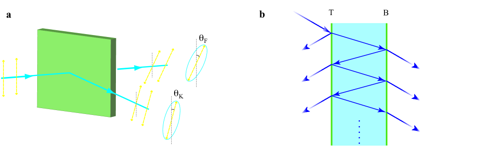
Figure 1: (Color online) (a). Schematic illustration of the Faraday and Kerr effects. Incident linearly polarized light becomes elliptically polarized after transmission (Faraday effect) and reflection (Kerr effect), with polarization plane angle rotations $\theta_{\mathrm{F}}$ and $\theta_{\mathrm{K}}$ respectively. (b) Fabry-Perot-like reflection and transmission in the TI film geometry. ‘T’ stands for the top surface and ‘B’ the bottom surface.

The original discussion of Wilzcek Wilczek imagined axion electrodynamics induced by a bulk spherical medium with a non-zero $\theta$ parameter separated from vacuum with $\theta=0$ by a single simply-connected surface. In the case of a spherical TI sample, this formulation can correctly capture the material’s surface Hall conductivity. Similarly, the case of an ideal semi-infinite TI slab SCZhangRev can be described by a topological field theory model with $\theta\neq 0$ in the topological insulator and $\theta=0$ in vacuum. In a magneto-optics setting, however, a propagating electromagnetic wave necessarily interacts with two nearby surfaces, since a real TI thin film sample has both top and bottom surfaces. Assuming that the mechanism that breaks time-reversal invariance at the TI surface does so in the same sense on both top and bottom, both surfaces will have the same Hall conductivity. In topological field theory, this would be captured by a model in which the discontinuity in $\theta$ in the direction of light propagation has the same sign and magnitude at both surfaces. To describe a thin film with identical half-quantized Hall conductivities on opposite surfaces it is then necessary to take $\theta=\pm 2\pi$ in one of the vacuum regions. A TI thin film model in which the surrounding material has $\theta=0$ everywhere would instead describe a system with opposite Hall conductivities on opposite surfaces. Because of the opposite contributions, the magneto-optical effects would then vanish for films thinner than a wavelength.

Given the surface massless Dirac models, our approach to magneto-electric properties is more conventional. Magneto-electric properties are completely determined by the conductivity of the material, including bulk and surface, longitudinal and Hall contributions. The role of the theta-term in axion electrodynamics equations is completely replaced by the appearance of explicit surface Hall conductivities that influence electromagnetic wave boundary conditions. These calculations make it clear that magneto-electric properties depend essentially on the numerical values of the surface conductivities, not just on whether they are quantized or half-quantized. This is especially important when surface time-reversal invariance is broken by an external magnetic field, since both the sign and the magnitude of the surface currents will be sensitive to the position of the Fermi level within the bulk gap. In addition to this advantage, the optical response of the surface Dirac fermions can be evaluated microscopically, enabling a natural incorporation of dynamical and many-body effects.

Interesting magneto-optical effects occur in both low-frequency and higher frequency regimes. In the latter case, we have found interband absorption Tse_1 and cyclotron resonance Tse_2 features in the Faraday and Kerr rotations that are dramatically enhanced by the cavity confinement effect of the TI thin film. We focus mainly on the large topological magneto-optical effects at low frequencies which can be observed only if the following conditions are satisfied: (1) The TI surface has a quantized Hall effect allowed by time-reversal breaking due to either external magnetic field or exchange coupling to external electronic degrees of freedom. We know from vast experience with the quantum Hall effect in an external magnetic field in graphene, which is also described by a massless Dirac equation, that the quantum Hall effect can occur at quite weak magnetic fields when the Fermi level is close to the Dirac point and disorder is very weak. Exchange-coupling to spin yields a half-quantized anomalous Hall effect in the absence of disorder Haldane ; QSH_Kane . Although there are no experimental examples of quantized anomalous Hall effect as yet, the requirements on time-reversal breaking perturbation strength in the presence of disorder are likely to be similar. The magneto-electric anomalies require large Hall effects at finite electromagnetic wave frequency. This condition requires that the frequency be much smaller than the surface gap. (2) The dimension of the TI along the direction of light travel should be shorter than the electromagnetic wavelength or a nonzero integer multiple of the half wavelength. In either case, the dielectric properties of the TI bulk medium that separates the two quantized Hall layers do not influence the transmitted and reflected light. When these conditions are satisfied, the magneto-optical effects are universal and topologically protected against weak surface disorder.

The outline of our paper is as follows. In the Section II, we review linear response theory for the optical conductivity tensor of TI surface helical quasiparticles. In Section III, we summarize the electromagnetic scattering formalism appropriate for a system with two metallic surfaces surrounded by dielectrics, applicable to TI films and to other similar layered systems. We then present and discuss our results for the magneto-optical Faraday and Kerr effects, first for TI films that are thinner than a wavelength and then for the general case. In Section V we address some issues pertinent to experiments including the influence of bulk conduction, the role of oblique incidence, and the role of substrates. Finally in Section VI we discuss the closely related magneto-optical properties of graphene-based layered massless Dirac systems.

II Dynamical Response of a Spin-Helical Dirac Fermions

We first derive explicit analytic expressions for the longitudinal and Hall optical conductivities of the spin-helical quasiparticles of topological insulator surfaces with time-reversal symmetry broken in two different ways: (1) an exchange field that couples to spin, and (2) an external magnetic field that couples to both spin and orbital degrees of freedom. The former case can be realized by exchange coupling between the TI surface and an adjacent ferromagnetic insulator Tse_1 ; SCZhangRev . The response of TI surface carriers to exchange coupling is unique, and ongoing progress along this direction has been reported by several experimental groups Hasan_doping1 ; Hasan_doping2 ; Shen_doping ; Cui_doping .

In the presence of time-reversal symmetry breaking, the massless Dirac Hamiltonians for the top (T) and bottom (B) surfaces are

$$H=(-1)^{L}\;[v\bm{\tau}\cdot(-i\nabla+e\bm{A}/c)+V/2]+\Delta\tau_{z},$$ (1)

where $\bm{\tau}$ is the spin Pauli matrix vector (expressed in $90^{\circ}$ rotated basis from the real spins spindirection ), $\bm{A}$ is the magnetic vector potential, $\Delta$ is the Zeeman coupling strength, $V$ accounts for a possible potential difference between top and bottom surfaces due to doping or external gates, and $L=0,1$ for the top ($0$) and bottom ($1$) surfaces. Note that in spite of the sign difference in the kinetic energy terms for the top and bottom surfaces, the conductivities are identical on the two surfaces. The massless Dirac surface states description is valid for energies below the energy cut-off of the Dirac Hamiltonian $\varepsilon_{\mathrm{c}}$, which we associate with the separation between the Dirac point and the closest bulk band.

II.1 Exchange Field

Time-reversal symmetry breaking by an exchange field can be realized by interfacing the TI surface with an insulating ferromagnet with magnetization oriented perpendicularly. Magnetic proximity coupling with strength $\Delta$ will favor alignment of the TI surface spins. The numerical value of $\Delta$ would be determined by the orbital hybridization between the ferromagnetic material and the TI surface. $A=0$ in Eq. (1) in the absence of an applied magnetic field. In this limit, the Dirac cone is gapped with conduction ($\mu=1$) and valance ($\mu=-1$) band dispersions and eigenstates

$$\varepsilon_{k\mu}=\mu\varepsilon_{k},\,\,\,\,\,|k\mu\rangle=\begin{bmatrix}C_{\uparrow k\mu}\\ C_{\downarrow k\mu}e^{i\phi_{k}}\end{bmatrix}.$$ (2)

where $\varepsilon_{k}=\sqrt{(vk)^{2}+\Delta^{2}}$, $\phi_{k}$ is the azimuthal angle of the crystal momentum, and

$$C_{\uparrow k\mu} = \mathrm{sgn}(\mu)\sqrt{\varepsilon_{k}+\mathrm{sgn}(\mu)\Delta}/\sqrt{2\varepsilon_{k}},$$

$$C_{\downarrow k\mu} = \sqrt{\varepsilon_{k}-\mathrm{sgn}(\mu)\Delta}/\sqrt{2\varepsilon_{k}},$$ (3)

The optical conductivity tensor of the helical quasiparticles on topological insulator surface can be obtained from the Kubo formula:

$$\sigma_{\alpha\beta}\left(\omega\right)=ig\sum_{k}\sum_{\mu\mu^{\prime}}\frac{f_{k\mu}-f_{k\mu^{\prime}}}{\varepsilon_{k\mu}-\varepsilon_{k\mu^{\prime}}}\frac{\langle k\mu|j_{\alpha}|k\mu^{\prime}\rangle\langle k\mu^{\prime}|j_{\beta}|k\mu\rangle}{\omega+\varepsilon_{k\mu}-\varepsilon_{k\mu^{\prime}}+i/2\tau_{\mathrm{s}}},$$ (4)

where $\alpha,\beta=\{x,y\}$, $\mu,\mu^{\prime}=\pm 1$ denote the band index, $f_{k\mu}$ is the Fermi factor for band $\mu$, $1/\tau_{\mathrm{s}}$ is the quasiparticle lifetime broadening of the surface states, and $g$ is the (odd) number of Dirac cones on the TI surface, which we take for simplicity and concreteness to be $1$. This expression is not quantitatively correct when disorder is present (i.e. when $\tau_{\mathrm{s}}$ is finite), because it does not capture the localization physics that is important in the quantum Hall regime, but it is adequate for our present interest. We evaluate the longitudinal conductivity $\sigma_{xx}(\omega)=\sigma_{xx}^{\mathcal{R}}+i\sigma_{xx}^{\mathcal{I}}$ and the Hall conductivity $\sigma_{xy}(\omega)=\sigma_{xy}^{\mathcal{R}}+i\sigma_{xy}^{\mathcal{I}}$ in the topological transport regime when the Fermi level lies within the TRS breaking gap. Since all surface optical conductivities eventually appear in the outgoing electromagnetic fields in the combination $\sigma_{\alpha\beta}/c$, we shall adopt the ‘natural units’ for the optical conductivities and express ${\sigma}_{\alpha\beta}$ in $e^{2}/\hbar=\alpha\,c$ units ($\alpha=1/137$ is the vacuum fine structure constant) and set $c=1$ except where specified. For the dissipative components of the optical conductivity we find that:

$$\sigma_{xx}^{\mathcal{R}} = \frac{1}{16\pi x(\omega^{2}+\Gamma^{2})^{2}}$$

$$\times\left\{x\left[(\omega^{2}+\Gamma^{2})^{2}+4(\omega^{2}-\Gamma^{2})\Delta^{2}\right]g(x)\right.$$

$$\left.+4\Gamma\Delta^{2}\left[\omega^{2}+\Gamma^{2}+\omega xf(x)\right]\right\}\big{|}_{x=\Delta}^{x=\varepsilon_{\mathrm{c}}}$$

$$\sigma_{xy}^{\mathcal{I}} = \frac{\Delta}{8\pi(\omega^{2}+\Gamma^{2})}\left[-2\omega g(x)-\Gamma f(x)\right]\big{|}_{x=\Delta}^{x=\varepsilon_{\mathrm{c}}}$$ (5)

For the reactive, non-dissipative components of the optical conductivity $\sigma_{xx}^{\mathcal{I}}$ and $\sigma_{xy}^{\mathcal{R}}$, which are due to off-shell virtual transitions, we find that:

$$\sigma_{xx}^{\mathcal{I}} = \frac{1}{32\pi x(\omega^{2}+\Gamma^{2})^{2}}\left\{8\omega\Delta^{2}(\omega^{2}+\Gamma^{2})-16x\omega\Gamma\Delta^{2}g(x)\right.$$

$$\left.+x\left[(\omega^{2}+\Gamma^{2})^{2}+4\Delta^{2}(\omega^{2}-\Gamma^{2})\right]f(x)\right\}\big{|}_{x=\Delta}^{x=\varepsilon_{\mathrm{c}}}$$

$$\sigma_{xy}^{\mathcal{R}} = \frac{\Delta}{8\pi(\omega^{2}+\Gamma^{2})}\left[-2\Gamma g(x)+\omega f(x)\right]\big{|}_{x=\Delta}^{x=\varepsilon_{\mathrm{c}}}$$

where $R(x)|_{x=x_{1}}^{x=x_{2}}$ means $R(x_{2})-R(x_{1})$, $\Gamma=1/2\tau_{\mathrm{s}}$, and

$$f(x) = \mathrm{ln}\left|\frac{(\omega-2x)^{2}+\Gamma^{2}}{(\omega+2x)^{2}+\Gamma^{2}}\right|,$$

$$g(x) = \tan^{-1}\left(\frac{\omega-2x}{\Gamma}\right)-\tan^{-1}\left(\frac{\omega+2x}{\Gamma}\right).$$ (7)

When the disorder broadening is small such that $\Gamma\ll\Delta$, it is useful to obtain analytic results in the disorder-free limit $\Gamma\to 0$, in which case

$$g(x)\big{|}_{x=\Delta}^{x=\varepsilon_{\mathrm{c}}}=-\pi\theta(|\omega|-2|\Delta|),$$ (8)

and Eqs. (5)-(7) reduce to our previous results [Eqs. (2)-(3) in Ref. Tse_1, ] obtained from the quantum kinetic equation approach.

II.2 External Quantizing Magnetic Field

Landau level (LL) quantization of the TI’s surface Dirac cones has recently been observed by STM experiments STM1 ; STM2 . In the presence of a quantizing field, the vector potential in Eq. (1) is given in the Landau gauge by $\bm{A}=(0,Bx)$ and the Zeeman coupling by $\Delta=g_{\mathrm{J}}\mu_{\mathrm{B}}B/2$, where $g_{\mathrm{J}}$ is the electron g factor. Define raising and lowering operators $a=(\ell_{B}/\sqrt{2})[\partial_{x}+(x+x_{0})/\ell_{B}^{2}]$ and $a^{\dagger}=(\ell_{B}/\sqrt{2})[-\partial_{x}+(x+x_{0})/\ell_{B}^{2}]$ with $\ell_{B}=1/\sqrt{e|B|}$ the magnetic length and $x_{0}=k_{y}\ell_{B}^{2}$ the guiding center coordinate, Eq. (1) can be written as

$$\begin{bmatrix}{\Delta}&-i\left({\sqrt{2}v}/{\ell_{B}}\right)a\\ i\left({\sqrt{2}v}/{\ell_{B}}\right)a^{\dagger}&-{\Delta}\end{bmatrix}|\overline{n}\rangle=\varepsilon|\overline{n}\rangle,$$ (9)

where $|\overline{\cdots}\rangle$ denotes an eigenspinor. The LLs are labeled by integers $n$ and for $n\neq 0$ and have eigenenergies [relative to the respective Dirac point energies $(-1)^{L}V/2$] and eigenspinors

$$\varepsilon_{n}=\mathrm{sgn}(n)\sqrt{\frac{2v^{2}}{\ell_{B}^{2}}|n|+\Delta^{2}},\,\,\,\,\,|\overline{n}\rangle=\begin{bmatrix}-i\mathcal{C}_{\uparrow n}||n|-1\rangle\\ \mathcal{C}_{\downarrow n}||n|\rangle\end{bmatrix}.$$ (10)

where $||n|\rangle$ without an overbar denotes a Fock state ($|n|$ is the absolute value of $n$), and

$$\mathcal{C}_{\uparrow n} = \mathrm{sgn}(n)\sqrt{\varepsilon_{|n|}+\mathrm{sgn}(n)\Delta}/\sqrt{2\varepsilon_{|n|}},$$

$$\mathcal{C}_{\downarrow n} = \sqrt{\varepsilon_{|n|}-\mathrm{sgn}(n)\Delta}/\sqrt{2\varepsilon_{|n|}}.$$ (11)

In the $n=0$ LL spins are aligned with the perpendicular field so that

$$\varepsilon_{0}=-\Delta,\,\,\,\,\,|\overline{0}\rangle=\begin{bmatrix}0\\ |0\rangle\end{bmatrix}.$$ (12)

In the quantum Hall regime ($\Omega_{B}\tau_{\mathrm{s}}\gg 1$ where $\Omega_{B}=v/\ell_{B}$ is a characteristic frequency typical of the LLs spacing), the conductivity tensor can be expressed in LL basis as

$$\sigma_{\alpha\beta}\left(\omega\right)=\frac{ig}{2\pi\ell_{B}^{2}}\sum_{nn^{\prime}}\frac{f_{n}-f_{n^{\prime}}}{\varepsilon_{n}-\varepsilon_{n^{\prime}}}\frac{\langle\overline{n}|j_{\alpha}|\overline{n^{\prime}}\rangle\langle\overline{n^{\prime}}|j_{\beta}|\overline{n}\rangle}{\omega+\varepsilon_{n}-\varepsilon_{n^{\prime}}+i/2\tau_{\mathrm{s}}},$$ (13)

where the current operator is $\bm{j}=ie\left[H,\bm{x}\right]=ev\bm{\tau}$. For convenience we rewrite the LL index as $n=sm$, where $m=0,1,2,\cdots N_{\mathrm{c}}$ and $s=\pm 1$ for electron-like and hole-like LLs. The current matrix element $\langle\overline{n}|j_{\alpha}|\overline{n^{\prime}}\rangle$ captures the selection rule $|n^{\prime}|-|n|=\pm 1$ for LL transitions. After some algebra we find that the conductivity tensor Eq. (13) in $e^{2}/\hbar=\alpha c$ units is given by

$$\sigma_{\alpha\beta}(\omega)=\frac{v^{2}}{2\pi\ell_{B}^{2}}\sum_{m=0}^{N_{\mathrm{c}}-1}\sum_{s,s^{\prime}=\pm 1}\frac{f_{sm}-f_{s^{\prime}(m+1)}}{\varepsilon_{sm}-\varepsilon_{s^{\prime}(m+1)}}\;\Gamma_{\alpha\beta}^{s,s^{\prime}}(m,\omega),$$

(14)

where

$$\Gamma_{\left\{\begin{subarray}{l}xx\\ xy\end{subarray}\right\}}^{s,s^{\prime}}(m,\omega)=-\left\{\begin{array}[]{c}i\\ 1\end{array}\right\}\mathcal{C}_{\uparrow s^{\prime}(m+1)}^{2}\mathcal{C}_{\downarrow sm}^{2}$$ (17)

$$\left(\frac{1}{\omega-\varepsilon_{sm}+\varepsilon_{s^{\prime}(m+1)}+i/2\tau_{\mathrm{s}}}\pm\frac{1}{\omega+\varepsilon_{sm}-\varepsilon_{s^{\prime}(m+1)}+i/2\tau_{\mathrm{s}}}\right).$$

In Eq.( 17), $N_{\mathrm{c}}\simeq\ell_{B}^{2}(\varepsilon_{\mathrm{c}}^{2}-\Delta^{2})/2v^{2}$ is the largest LL index with an energy smaller than the ultraviolet cut-off $\varepsilon_{\mathrm{c}}$, prefactor $i$ and sign ‘$+$’ inside the parenthesis apply to the $\Gamma_{xx}$ expression, $1$ and ‘$-$’ to the $\Gamma_{xy}$ expression. Eqs. (14)-(17) express $\sigma_{\alpha\beta}$ as a sum over interband and intraband dipole-allowed transitions which satisfy $|n^{\prime}|-|n|=\pm 1$. In the $\omega=T=\tau_{\mathrm{s}}^{-1}=0$ limit Eq. (14) yields correct half-quantized plateau values for the Hall conductivity.

III Light Propagation through a TI Slab

In this section, we formulate the problem of electromagnetic wave scattering through a topological insulator slab illustrated schematically in Fig. 1(b). Here we discuss only the normal incidence case. More general results for the oblique incidence case are presented in an Appendix.

Consider an electromagnetic wave propagating along the $z$ direction through two materials, labeled by $i$ and $j$, with dielectric constant and magnetic permeability $\epsilon_{i},\mu_{i}$ and $\epsilon_{j},\mu_{j}$ respectively. The interface between them is at $z=a_{i}$. We write the electric field component of the electromagnetic field in the form

$$\tilde{E}^{i}=e^{ik_{i}z}\left[\begin{array}[]{c}E_{x}^{ti}\\ E_{y}^{ti}\end{array}\right]+e^{-ik_{i}z}\left[\begin{array}[]{c}E_{x}^{ri}\\ E_{y}^{ri}\end{array}\right],$$ (22)

where the tilde accents denote vectors $\tilde{E}=[E_{x}\,\,\,E_{y}]^{\mathrm{T}}$, the superscripts ‘$\mathrm{r}$’ and ‘$\mathrm{t}$’ on $\tilde{E}$ denote the reflected and transmitted components of the electric field, and $k_{i}=(\omega/c)\sqrt{\epsilon_{i}\mu_{i}}$ is the wavevector in medium $i$. The corresponding magnetic field is given by Faraday’s law as

$$\tilde{H}^{i}=\sqrt{\frac{\epsilon_{i}}{\mu_{i}}}\left\{e^{ik_{i}z}\left[\begin{array}[]{c}-E_{y}^{ti}\\ E_{x}^{ti}\end{array}\right]+e^{-ik_{i}z}\left[\begin{array}[]{c}E_{y}^{ri}\\ -E_{x}^{ri}\end{array}\right]\right\},$$ (27)

The electric and magnetic fields at the interface $z=a_{i}$ satisfy the electrodynamic boundary conditions $\tilde{E}^{i}=\tilde{E}^{j}$ and $-i\tau_{y}(\tilde{H}^{j}-\tilde{H}^{i})=(4\pi/c)\tilde{J}^{i}$, where $\tau_{y}$ is the Pauli matrix and $\tilde{J}^{i}=\bar{\sigma}^{i}\tilde{E}^{i}$ is the surface current density at $z=a_{i}$. Note that this surface current can have longitudinal and Hall response components in this microscopic theory and not only Hall components as assumed in topological field theory.

The scattering matrix that relates incoming $[\tilde{E}^{\mathrm{t}i}\,\,\,\tilde{E}^{\mathrm{r}j}]^{\mathrm{T}}$ and outgoing $[\tilde{E}^{\mathrm{r}i}\,\,\,\tilde{E}^{\mathrm{t}j}]^{\mathrm{T}}$ fields at a conducting interface can be written in the form

$$S=\left[\begin{array}[]{cc}\bar{r}&\bar{t^{\prime}}\\ \bar{t}&\bar{r^{\prime}}\end{array}\right],$$ (28)

where the superscripts ‘$\mathrm{r}$’ and ‘$\mathrm{t}$’ on $\tilde{E}$ denote reflected and transmitted components of the electric fields, and $\bar{r},\bar{r^{{}^{\prime}}}$ and $\bar{t},\bar{t^{{}^{\prime}}}$ are $2\times 2$ reflection and transmission tensors, which are of the form:

$$\bar{r}=\begin{bmatrix}r_{xx}&r_{xy}\\ -r_{xy}&r_{yy}\end{bmatrix},\,\,\,\,\,\bar{t}=\begin{bmatrix}t_{xx}&t_{xy}\\ -t_{xy}&t_{yy}\end{bmatrix},$$ (29)

and similarly for $\bar{r^{{}^{\prime}}},\bar{t^{{}^{\prime}}}$. Matching boundary conditions, we obtain the following expressions for $\bar{r},\bar{t}$ $\bar{r}^{{}^{\prime}}$ and $\bar{t}^{{}^{\prime}}$:

$$\left\{\begin{array}[]{c}r_{xx}\\ r_{xy}\end{array}\right\}=\frac{e^{i2k_{i}a_{i}}}{(\sqrt{\epsilon_{i}/\mu_{i}}+\sqrt{\epsilon_{j}/\mu_{j}}+4\pi{\sigma}_{xx})^{2}+(4\pi{\sigma}_{xy})^{2}}$$ (32)

$$\times\left\{\begin{array}[]{c}\epsilon_{i}/\mu_{i}-(\sqrt{\epsilon_{j}/\mu_{j}}+4\pi{\sigma}_{xx})^{2}-(4\pi{\sigma}_{xy})^{2}\\ -8\pi\sqrt{\epsilon_{i}/\mu_{i}}{\sigma}_{xy}\end{array}\right\},$$ (35)

$$\left\{\begin{array}[]{c}t_{xx}\\ t_{xy}\end{array}\right\}=\frac{e^{i(k_{i}-k_{j})a_{i}}}{(\sqrt{\epsilon_{i}/\mu_{i}}+\sqrt{\epsilon_{j}/\mu_{j}}+4\pi{\sigma}_{xx})^{2}+(4\pi{\sigma}_{xy})^{2}}$$ (38)

$$\times\left\{\begin{array}[]{c}2\sqrt{\epsilon_{i}/\mu_{i}}(\sqrt{\epsilon_{i}/\mu_{i}}+\sqrt{\epsilon_{j}/\mu_{j}}+4\pi{\sigma}_{xx})\\ -8\pi\sqrt{\epsilon_{i}/\mu_{i}}{\sigma}_{xy}\end{array}\right\}.$$ (41)

For normal incidence, the two diagonal elements of the reflection and transmission matrices are identical: $r_{yy}^{(^{\prime})}=r_{xx}^{(^{\prime})}$ and $t_{yy}^{(^{\prime})}=t_{xx}^{(^{\prime})}$. $\bar{r^{\prime}}$ can be obtained from $\bar{r}$ by making the replacement $k_{i}\to-k_{j}$ and interchanging $\epsilon_{i}/\mu_{i}$ and $\epsilon_{j}/\mu_{j}$, and $\bar{t^{\prime}}$ from $\bar{t}$ by interchanging $\epsilon_{i}/\mu_{i}$ and $\epsilon_{j}/\mu_{j}$. In addition, $\bar{t}$ and $\bar{t}^{\prime}$ are related by $\bar{t}/\sqrt{\epsilon_{i}/\mu_{i}}=\bar{t}^{\prime}/\sqrt{\epsilon_{j}/\mu_{j}}$.

Scattering from a TI film presents an electromagnetic problem in which scattering occurs from two interfaces at which currents flow and dielectric constants are discontinuous. The reflection and transmission tensor can be composed from the single-interface scattering matrices $\bar{r^{(^{\prime})}},\bar{t^{(^{\prime})}}$ for the top and bottom surfaces to obtain

$$\bar{r} = \bar{r_{\mathrm{T}}}+\bar{t_{\mathrm{T}}^{\prime}}\bar{r_{\mathrm{B}}}\left(\bm{1}-\bar{r_{\mathrm{T}}^{\prime}}\bar{r_{\mathrm{B}}}\right)^{-1}\bar{t_{\mathrm{T}}},$$ (42)

$$\bar{t} = \bar{t_{\mathrm{B}}}\left(\bm{1}-\bar{r_{\mathrm{T}}^{\prime}}\bar{r_{\mathrm{B}}}\right)^{-1}\bar{t_{\mathrm{T}}}.$$ (43)

The presence of a dielectric substrate underneath the TI film is easily accounted for by propagating the reflection and transmission tensors Eqs. (42)-(43) through an additional layer of dielectric. Detailed expressions for the reflection and transmission tensors that allow for oblique incidence and account for a dielectric substrate are given in an Appendix.

IV Magneto-optical Faraday and Kerr Effects

For linearly polarized incoming light, the Faraday and Kerr angles can be defined in terms of the relative rotations of left-handed and right-handed circularly polarized light to obtain:

$$\theta_{\mathrm{F}} = \left(\mathrm{arg}\{E_{+}^{\mathrm{t}}\}-\mathrm{arg}\{E_{-}^{\mathrm{t}}\}\right)/2,$$ (44)

$$\theta_{\mathrm{K}} = \left(\mathrm{arg}\{E_{+}^{\mathrm{r}}\}-\mathrm{arg}\{E_{-}^{\mathrm{r}}\}\right)/2,$$ (45)

where ${E}_{\pm}^{\mathrm{r,t}}={E}_{x}^{\mathrm{r,t}}\pm i{E}_{y}^{\mathrm{r,t}}$ are the left-handed (+) and right-handed (-) circularly polarized components of the outgoing electric fields.

In this section, we present our results for an ideal topological insulator under normal light incidence. We then discuss non-ideal effects that may be relevant in experimental situations in Section V. It is important to emphasize that the magneto-optical effects are essentially the same in this limit for time-reversal symmetry broken by exchange coupling or by a quantizing magnetic field. In the case of a quantizing field, there are many gaps in the surface spectrum because of Landau quantization. The quantized Hall conductivity in $e^{2}/h$ units is equal to the filling factor $\nu_{\mathrm{T,B}}$. The largest gap in the magnetic field case occurs occurs at $\nu_{\mathrm{T,B}}=1/2$ and has the same Hall conductivity as for the Zeeman gap case. In the magnetic field case, it is possible to shift the Hall conductivities of either surface by integer multiples of $e^{2}/h$ away from $e^{2}/2h$ simply by shifting the position of the Dirac point relative to the chemical potential, and this shift would influence the magneto-optical effects. When the chemical potential is placed in the largest gap in the magnetic field case, the only differences between the two scenarios are in the details of the higher frequency response.

IV.1 Thin Film $d\ll\lambda$

First we consider the case of a TI film that is thinner than the light wavelength. In this limit it follows from Faraday’s law that the electric field is spatially constant across the film so that the two interfaces can be considered as one. Ampère’s Law implies that the magnetic field changes by a value proportional to the current integrated across the TI film,

$$-i\tau_{y}(\tilde{H}^{\mathrm{T}}-\tilde{H}^{\mathrm{B}})=(4\pi/c)\left(\bar{\sigma}_{\mathrm{T}}+\bar{\sigma}_{\mathrm{B}}\right)\tilde{E},$$ (46)

where $\tilde{H}^{\mathrm{T,B}}$ denotes the magnetic fields in the top and bottom vacuum regions outside of the film. Eq. (46) says that, from the viewpoint of the long electromagnetic wave, the TI film behaves effectively as a single two-dimensional surface with a conductivity equal to the conductivities integrated across the film. We therefore obtain the transmitted and reflected fields

$$\tilde{E}^{\mathrm{t}} = \frac{1}{\left(2+4\pi\sigma_{xx}\right)^{2}+\left(4\pi\sigma_{xy}\right)^{2}}\begin{bmatrix}4\left(1+2\pi\sigma_{xx}\right)\\ 8\pi\sigma_{xy}\end{bmatrix},$$ (47)

$$\tilde{E}^{\mathrm{r}} = \frac{1}{\left(2+4\pi\sigma_{xx}\right)^{2}+\left(4\pi\sigma_{xy}\right)^{2}}$$ (48)

$$\begin{bmatrix}1-\left(1+4\pi\sigma_{xx}\right)^{2}-\left(4\pi\sigma_{xy}\right)^{2}\\ 8\pi\sigma_{xy}\end{bmatrix},$$

for simplicity here we use $\sigma_{xx},\sigma_{xy}$ to denote the total longitudinal and Hall conductivities from both surfaces, respectively. An important observation is that in this limit the transmitted and reflected fields are independent of the bulk dielectric properties of the TI film. For weak disorder and frequencies much smaller than characteristic transition frequencies ($\omega\ll\Delta$ for the exchange field case and $\omega\ll\Omega_{B}$ for the magnetic field case), the optical conductivity has only a dissipationless DC Hall conductivity contribution:

$$\sigma_{xy}^{\mathcal{R}}=\frac{\nu_{\mathrm{T,B}}}{2\pi},$$ (49)

and $\sigma_{xx}^{\mathcal{R}}=\sigma_{xx}^{\mathcal{I}}=0$, $\sigma_{xy}^{\mathcal{I}}=0$. In this low-frequency regime, the magneto-optical response of the exchange field case becomes a special case of the quantizing magnetic field case with $\nu_{\mathrm{T}}=\nu_{\mathrm{B}}=1/2$ as explained above.

From Eqs. (47)-(48) we find the Faraday and Kerr angles

$$\theta_{\mathrm{F}}=\tan^{-1}\left[\left(\nu_{\mathrm{T}}+\nu_{\mathrm{B}}\right)\alpha\right],$$ (50)

$$\theta_{\mathrm{K}}=-\tan^{-1}\left[\frac{1}{\left(\nu_{\mathrm{T}}+\nu_{\mathrm{B}}\right)\alpha}\right].$$ (51)

For total filling factor $\nu_{\mathrm{T}}+\nu_{\mathrm{B}}$ values that are not too large, the Faraday angle is quantized in integer multiples of the fine structure constant

$$\theta_{\mathrm{F}}\simeq(\nu_{\mathrm{T}}+\nu_{\mathrm{B}})\alpha,$$ (52)

and the Kerr angle

$$\theta_{\mathrm{K}}=-\frac{\pi}{2},$$ (53)

becomes a full quarter polarization rotation.

It is also possible to understand Eq. (53) in terms of the scattering mechanism of the reflected partial wave components. This understanding is crucial to see that Eq. (53) applies over a finite frequency range, as discussed in Section V B. The reflected electric field can be easily found from Eq. (42). The algebra is simplified and the physics underlying Eq. (53) more easily illustrated when spatial-inversion symmetry across the TI film is preserved, i.e. when top and bottom surfaces have the same conductivities. This happens when the exchange fields for both surfaces are the same, or in the quantizing magnetic field case, when the surface densities (and thus filling factors) are the same. Spatial-inversion symmetry then implies that $\bar{r_{\mathrm{B}}}=\bar{r_{\mathrm{T}}}^{\prime}$, $\bar{r_{\mathrm{T}}}=\bar{r_{\mathrm{B}}}^{\prime}$, $\bar{t_{\mathrm{B}}}=\bar{t_{\mathrm{T}}}^{\prime}$, and $\bar{t_{\mathrm{T}}}=\bar{t_{\mathrm{B}}}^{\prime}$. This allows the reflected electric field to be expressed solely in terms of the reflection and transmission matrix elements of one (e.g., the top) of the two surfaces. The first term on the right hand side of Eq. (42) represents the partial wave directly reflected from the top surface, which we can evaluate in the low-frequency regime as

$$\tilde{E}^{\mathrm{r}0}=\frac{1}{\left(1+\sqrt{\epsilon/\mu}\right)^{2}+\left(4\pi\sigma_{xy}^{\mathcal{R}}\right)^{2}}\begin{bmatrix}1-\epsilon/\mu-\left(4\pi\sigma_{xy}^{\mathcal{R}}\right)^{2}\\ 8\pi\sigma_{xy}^{\mathcal{R}}\end{bmatrix},$$

(54)

where $\epsilon$, $\mu\simeq 1$ are the bulk dielectric constant and magnetic permeability of the TI, and the second term constitutes all the partial waves that originate from successive reflections from the bottom surface

$$\tilde{E}^{\mathrm{r}^{\prime}} = \frac{1}{1+\left(4\pi\sigma_{xy}^{\mathcal{R}}\right)^{2}}\begin{bmatrix}1\\ {4\pi\sigma_{xy}^{\mathcal{R}}}\end{bmatrix}$$

$$-\frac{1}{\left(1+\sqrt{\epsilon/\mu}\right)^{2}+\left(4\pi\sigma_{xy}^{\mathcal{R}}\right)^{2}}\begin{bmatrix}{2\left(1+\epsilon/\mu\right)}\\ {8\pi\sigma_{xy}^{\mathcal{R}}}\end{bmatrix}.$$

Summing the two contributions, we find that part of the second term on the right-hand side of Eq. (IV.1) cancels out the first term on the right-hand side of Eq. (54) completely, yielding a total reflected field

$$\tilde{E}^{\mathrm{r}}=\frac{1}{1+\left(4\pi\sigma_{xy}^{\mathcal{R}}\right)^{2}}\begin{bmatrix}-\left(4\pi\sigma_{xy}^{\mathcal{R}}\right)^{2}\\ 4\pi\sigma_{xy}^{\mathcal{R}}\end{bmatrix}.$$ (56)

Eq. (56) implies that the reflected partial waves that originate from successive scattering off the bottom surface destructively interfere with the partial wave scattered off the top surface, resulting in a suppression by a factor $\sim(\sigma_{xy}^{\mathcal{R}})^{2}$ of the reflected electric field component along the incident polarization direction. This leads to the giant Kerr angle in Eq. (53). It is worthwhile to make clear that the large Kerr angle occurs because almost all of the reflected partial waves have a $90^{\circ}$ rotated polarization plane; it is not true, however, that almost all of the light is reflected.

IV.2 Thick Film $d\gtrsim\lambda$

In the previous section, we have focused on films with a thickness that is only a fraction of the wavelength. In this section, we shall relax this assumption and generalize our considerations to thicker films, with thickness comparable to or greater than the wavelength inside the film. Thick films do not in general show spectacular magneto-optical effects because the Faraday and Kerr angles are suppressed by the large dielectric constant of the TI bulk. Exceptions occur when the film thickness contains an integer multiple of half wavelengths inside the film, i.e. when the cavity resonance condition $k_{\mathrm{TI}}d=N\pi$ is satisfied. Here $k_{\mathrm{TI}}=\sqrt{\epsilon\mu}\,\omega/c$ is the wave number in the TI film and $N\neq 0$ is an integer. This property was first identified in Ref. [QiBulkSubstrate, ], however the discussion there assumed an infinitely thick dielectric substrate underneath the TI film, neglecting scattering from the inevitable substrate-vacuum interface and thereby overestimating substrate suppression of magneto-optical responses. In this section, we first consider a free-standing thick film. We will then study the influence of a substrate, with its finite thickness properly accounted for, in Section V.

At resonance, a standing wave is established inside the film with the tangential components of the electric and magnetic fields on the interior of the top and bottom surfaces inside the film related simply by a $\pm$ sign, i.e. $E_{\parallel}(z=-d/2^{+})/E_{\parallel}(z=d/2^{-})=(-1)^{N}$ (here $z=0$ is taken at the center of the film), and similarly for $H$. Under such circumstances, the transmitted and reflected electric fields become independent of the film’s bulk dielectric properties, and are found to be given by Eqs. (47)-(48) multiplied by a phase factor $e^{-ik_{0}d}$, where $k_{0}=\omega/c$ is the vacuum wave number. In contrast to the long-wavelength regime we considered earlier in which the electromagnetic field varies slowly across the TI film, at resonance the field amplitudes change rapidly inside the film and the adiabatic condition $k_{0}d\ll 1$ does not apply. Regardless of the film thickness, however, the adiabaticity of TI surface electronic response can always be established at a sufficiently low frequency satisfying $\omega_{N}\ll\Delta$ or $\Omega_{\mathrm{B}}$ [$\omega_{N}=N\pi c/(\sqrt{\epsilon\mu}\,d)$ is the cavity resonance frequency], such that the quantum Hall condition Eq. (49) still holds. It follows from these considerations that the phases of the left-handed and right-handed circularly polarized components of the transmitted and reflected light are given by

$$\mathrm{arg}(E_{\lambda}^{\mathrm{t}}) = \frac{-{\lambda}\sin(k_{0}d)+2\pi\cos(k_{0}d)\sigma_{xy}^{\mathcal{R}}}{{\lambda}\cos(k_{0}d)+2\pi\sin(k_{0}d)\sigma_{xy}^{\mathcal{R}}},$$ (57)

$$\mathrm{arg}(E_{\lambda}^{\mathrm{r}}) = \frac{\cos(k_{0}d)+{\lambda}2\pi\sin(k_{0}d)\sigma_{xy}^{\mathcal{R}}}{\sin(k_{0}d)-{\lambda}2\pi\cos(k_{0}d)\sigma_{xy}^{\mathcal{R}}},$$ (58)

where $\lambda=\pm 1$ labels the left and right-handed circularly polarized light, and $\sigma_{xy}^{\mathcal{R}}$ contains the sum of the top and bottom surface Hall conductivities.

Let us make several remarks here. If we set $k_{0}d\to 0$, Eqs. (57)-(58) coincide with the long-wavelength ($k_{0}d<k_{\mathrm{TI}}d\ll 1$) results, from which we recover Eqs. (50)-(51) for the Faraday and Kerr angles. In general, if in addition to the requirement $k_{\mathrm{TI}}d=N\pi$ for resonance we also have $k_{0}d=M\pi$, then Eqs. (57)-(58) would imply that $\theta_{\mathrm{F}}=\tan^{-1}\left[\left(\nu_{\mathrm{T}}+\nu_{\mathrm{B}}\right)\alpha\right]$ and $\theta_{\mathrm{K}}=-\tan^{-1}\left[1/\left(\nu_{\mathrm{T}}+\nu_{\mathrm{B}}\right)\alpha\right]$ for integer $M$, and $\theta_{\mathrm{F}}=-\tan^{-1}\left[1/\left(\nu_{\mathrm{T}}+\nu_{\mathrm{B}}\right)\alpha\right]$ and $\theta_{\mathrm{K}}=\tan^{-1}\left[\left(\nu_{\mathrm{T}}+\nu_{\mathrm{B}}\right)\alpha\right]$ for half-odd integer $M$. These conditions would require $\sqrt{\epsilon\mu}=N/M$. With real materials this would seem to be rather impossible, however with the advent of metamaterials it may be possible to engineer one with a matching dielectric constant $(N/M)^{2}$, and employ it as an intervening dielectric between two single-layer graphene sheets. This point will be discussed further in Section VI. In this light, we see that the long-wavelength limit $k_{0}d<k_{\mathrm{TI}}d\to 0$ is special because it automatically satisfies both conditions $k_{\mathrm{TI}}d=N\pi$ and $k_{0}d=M\pi$ with $N=M=0$.

When $k_{0}d$ is not equal to a multiple of integer or half-odd integer of $\pi$, which is generally the case, only the cavity resonance condition is satisfied and $k_{0}d$ cannot be assumed as small in Eqs. (57)-(58). Evaluating $\theta_{\mathrm{F}}$ and $\theta_{\mathrm{K}}$ from Eqs. (44)-(45) using Eqs. (57)-(58), we find that the Faraday and Kerr rotations at resonance have the same universal quantized value

$$\theta_{\mathrm{F,K}}=\tan^{-1}\left[\left(\nu_{\mathrm{T}}+\nu_{\mathrm{B}}\right)\alpha\right].$$ (59)

Note that Eqs. (57)-(59) do not depend on the value of $N$ and therefore all cavity resonant modes yield the same Faraday and Kerr rotations given by Eq. (59). It is important to emphasize, at resonance, that although the Faraday angle is the same as the long-wavelength result Eq. (50), the Kerr angle is not given Remark1 by Eq. (51). Rather, both the Faraday and Kerr rotations at resonance are given by the same quantized response in units of $\alpha$ like Eq. (50). The giant Kerr effect Eq. (53), therefore, is a unique long-wavelength low-frequency property of the thin film system only.

V Deviations from an Ideal Topological Insulator Film

Magneto-optical measurements of Faraday and Kerr rotations produced by topological insulators Drew ; Armitage ; Molenkamp subjected to an external magnetic field have been performed by several groups. The samples studied include bulk Bi₂Se₃ crystals Drew , thin Bi₂Se₃ films Armitage and strained HgTe films Molenkamp . It has not yet been possible to achieve ideal samples in which the half-quantized quantum Hall effect occurs, either in DC transport or optically. In this section we consider non-ideal factors that often arise in experimental TI samples, and explain their consequences when they act independently. We focus on the influence of bulk carriers, light scattering at oblique incidence, and the influence of a dielectric substrate.

V.1 Influence of Bulk Carrier Conduction

Real TI samples are complicated by the presence of bulk free carriers which are present because of unintentional doping by bulk defects Transport1 ; Transport2 ; Transport3 ; Transport4 . Recently some progress has been reportedOh1 in reducing the density of bulk carriers in TI thin films.

Bulk conduction can be described by a complex bulk dielectric function $\epsilon(\omega)$ which is related to the bulk conductivity $\Sigma(\omega)$ by

$$\epsilon(\omega)=\epsilon_{\mathrm{b}}+i\frac{4\pi}{\omega}\Sigma(\omega),$$ (60)

where $\epsilon_{\mathrm{b}}$ is the high-frequency dielectric constant of the TI. When the quantized Hall regime is approached on the TI surfaces, the bulk Hall angle $\tan^{-1}(\Sigma_{xy}/\Sigma_{xx})$ is expected to be much smaller than the surface Hall angle (which becomes infinite when $\sigma_{xx}\to 0$). For definiteness the numerical results reported below assume that the longitudinal bulk conductivity dominates, and that its frequency-dependence can be described by the Drude-Lorentz form,

$$\Sigma(\omega)=\frac{\Omega_{\mathrm{b}}^{2}}{4\pi\left(1/\tau_{\mathrm{b}}-i\omega\right)},$$ (61)

where $\Omega_{\mathrm{b}}=\sqrt{{4\pi N_{\mathrm{b}}e^{2}}/{m_{\mathrm{b}}}}$ is the plasma frequency of the bulk carriers (with density $N_{\mathrm{b}}$ and effective mass $m_{\mathrm{b}}$), and $1/\tau_{\mathrm{b}}$ is the disorder scattering rate due to impurities present in the bulk.

The influence of a finite bulk conductivity is particularly simple to describe in the long-wavelength low-frequency limit of Eqs. (47)-(48). The total current integrated across the TI film in Eq. (46) now picks up an extra bulk conductivity contribution given by $\Sigma d$ ($d$ is the film thickness), in addition to the conductivities from the two surfaces. The change in the expressions for the transmitted and reflected electric fields Eqs. (47)-(48) is therefore altered by the replacement $\sigma_{xx}\to\sigma_{xx}+\Sigma d/c$. When the surface has a perfect quantum Hall effect, the modified expressions for the Faraday and Kerr angles are

$$\theta_{\mathrm{F}} = \tan^{-1}\left[\frac{\left(\nu_{\mathrm{T}}+\nu_{\mathrm{B}}\right)\alpha}{1+2\pi\Sigma d/c}\right],$$ (62)

$$\theta_{\mathrm{K}} = \tan^{-1}\left\{\frac{4\left(\nu_{\mathrm{T}}+\nu_{\mathrm{B}}\right)\alpha}{1-(1+4\pi\Sigma d/c)^{2}-[2\left(\nu_{\mathrm{T}}+\nu_{\mathrm{B}}\right)\alpha]^{2}}\right\},$$

where $\Sigma=\Sigma(0)$ is the bulk DC conductivity. The bulk carriers thus enter as an effective longitudinal surface conductivity $\Sigma d$. Eq. (62) implies that the influence of bulk conduction is negligible on the Faraday effect when

$$\frac{\Sigma d}{(e^{2}/h)}\ll 1/\alpha.$$ (64)

For the Kerr effect, Eq. (LABEL:Kerrw0_bulk) implies a stricter condition for negligible bulk conduction:

$$\frac{\Sigma d}{(e^{2}/h)}\lesssim\alpha.$$ (65)

When the bulk conductivity is sufficiently small that Eq. (65) is satisfied, Eqs. (62)-(LABEL:Kerrw0_bulk) reduce to the universal results for the Faraday and Kerr effects, Eqs. (50)-(53).

Eq. (65) can alternately can be expressed as a condition that has to be satisfied by the bulk carrier density:

$$N_{\mathrm{b}}\lesssim\frac{\alpha m_{\mathrm{b}}}{h\tau_{\mathrm{b}}d}.$$ (66)

For a $30$-nm thick Be₂Se₃ film and disorder broadening $\hbar/\tau_{\mathrm{b}}=1-10\,\mathrm{meV}$, we estimate that the to observe the giant Kerr effect, the bulk carrier density must be smaller than $10^{14}\,-\,10^{15}\,\mathrm{cm}^{-3}$. To reach the regime of the quantized Faraday effect given by Eq. (64), the bulk carrier density is allowed to be larger by a factor $1/\alpha^{2}$ so that $N_{\mathrm{b}}\lesssim{m_{\mathrm{b}}}/({\alpha h\tau_{\mathrm{b}}d})\simeq 10^{18}\,-\,10^{19}\,\mathrm{cm}^{-3}$. Fig 2 shows the low-frequency Kerr angle in the presence of bulk conduction. The magneto-optical response is modified by the presence of bulk carriers principally in the low frequency regime where the bulk Drude-Lorentz conductivity is peaked.

Because bulk carriers originate from bulk defects, $N_{\mathrm{b}}$ and $\tau_{\mathrm{b}}$ are related. For the purpose of studying their influence on the magneto-optical response we will nevertheless treat $N_{\mathrm{b}}$ and $\tau_{\mathrm{b}}$ as independent parameters. We first illustrate the case when there are no impurities in the bulk, i.e. the case of a bulk free plasma. We find that the giant Kerr angle remains but undergoes a shift to progressively higher frequencies for increasing bulk carrier density [Fig. 2 (a)]. Including bulk impurities broadens [Figs. 2 (b)-(c)] the giant Kerr effect, but the Kerr angle remains substantial $\sim 1\,\mathrm{rad}$ for a bulk density $N_{\mathrm{b}}=10^{17}\,\mathrm{cm}^{-3}$ and disorder broadening $\hbar/\tau_{\mathrm{b}}=1-10\,\mathrm{meV}$.

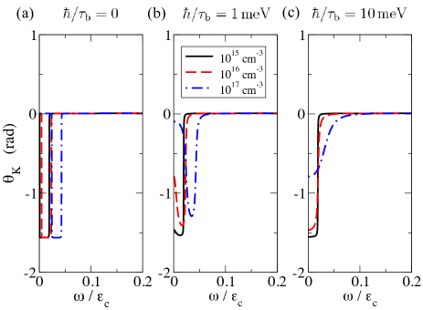
Figure 2: (Color online) Kerr rotation for top and bottom surface densities $n_{\mathrm{T}}=n_{\mathrm{B}}=3\times 10^{11}\,\mathrm{cm}^{-2}$ and filling factors $\nu_{\mathrm{T}}=\nu_{\mathrm{B}}=1/2$ (corresponding to a magnetic field of $25\,\mathrm{T}$) for (a) no bulk carrier scattering (b) $\hbar/\tau_{\mathrm{b}}=1\,\mathrm{meV}$, and (c) $10\,\mathrm{meV}$ at different values of bulk carrier densities $N_{\mathrm{b}}=10^{15}\,\mathrm{cm}^{-3}(\textrm{black solid line})$, $10^{16}\,\mathrm{cm}^{-3}(\textrm{red dashed})$, $10^{17}\,\mathrm{cm}^{-3}(\textrm{blue dot-dashed})$. The dielectric constant of Bi₂Se₃ $\epsilon_{\mathrm{b}}=29$, bulk carrier effective mass $m_{\mathrm{b}}=0.15m_{e}$ Transport4 ; Eto ; Butch , film thickness $d=30\,\mathrm{nm}$.

For thick films, we note that the presence of bulk conduction the cavity resonance condition becomes non-trivial. For this reason there is no simple analytic criterion for neglecting the bulk conductivity. Experimentally, this may also present a challenge since resonance frequencies cannot be readily estimated unless the bulk conductivity is known from a separate transport measurement.

In passing, we mention that bulk optical phonon modes of the topological insulator can also be excited at higher frequencies. Since phonon energies are specific to different TI materials and we are mainly interested in the low-frequency regime for the magneto-optical effects, we shall neglect the bulk optical phonon contributions to the conductivity. Phonon effects can be modeled by including an additional term Drew ; Armitage

$$\epsilon_{\mathrm{ph}}(\omega)=\frac{f_{\mathrm{ph}}}{{\omega_{\mathrm{ph}}}^{2}-\omega^{2}-i\omega/2\tau_{\mathrm{ph}}},$$ (67)

to the dielectric constant Eq. (60), where $f_{\mathrm{ph}}$ is the spectral weight of the phonon mode with frequency $\omega_{\mathrm{ph}}$, and $1/2\tau_{\mathrm{ph}}$ is the phonon damping rate. This separation between the electronic and the phononic contributions to the bulk dielectric function applies only when the electronic time scales ($\Omega_{\mathrm{b}}^{-1},\varepsilon_{F\mathrm{b}}^{-1}$, where $\varepsilon_{F\mathrm{b}}$ is the bulk Fermi energy) are much smaller than the phonon time scale ($\omega_{\mathrm{ph}}^{-1}$), making plasmon-phonon coupling negligible.

V.2 Influence of Oblique Incidence and the Substrate

In this section, we examine the effects of oblique incidence and of the substrate on the magneto-optical effects. This discussion is particularly germane to experiments because oblique incidence may afford an advantage over normal incidence for Kerr effect measurement as it allows for spatial separation between the incident light source and the reflected light polarizer, and enhances the reflected light intensity.

V.2.1 Thin TI Film and Thin Substrate

We now account for a dielectric substrate layer underneath the TI film and allow for the (semi-infinite) medium underneath the substrate to be different from vacuum, solely for generality. The incident angle on the TI film and the emerging angle from the substrate can therefore assume different values, denoted by $\theta_{\mathrm{i}}$ and $\theta_{\mathrm{o}}$ respectively. At low frequencies ($\omega\ll\Delta$ or $\Omega_{B}$) and long wavelength compared to both the film thickness $d$ and substrate thickness $d_{\mathrm{s}}$, the analysis is again simple. We find the following Faraday and Kerr angles under oblique incidence (Expressions for the transmission and reflection coefficients at oblique incidence are presented in the Appendix.):

$$\theta_{\mathrm{F}}=\mathrm{tan}^{-1}\left[\frac{2\alpha(\nu_{\mathrm{T}}+\nu_{\mathrm{B}})\mathrm{cos}\theta_{\mathrm{i}}}{\mathrm{cos}\theta_{\mathrm{i}}+\mathrm{cos}\theta_{\mathrm{o}}}\right],$$ (68)

$$\theta_{\mathrm{K}}=$$ (69)

$$-\mathrm{tan}^{-1}\left[\frac{8\alpha(\nu_{\mathrm{T}}+\nu_{\mathrm{B}})\mathrm{cos}\theta_{\mathrm{i}}\mathrm{cos}\theta_{\mathrm{o}}}{\mathrm{cos}2\theta_{\mathrm{o}}-\mathrm{cos}2\theta_{\mathrm{i}}+8\alpha^{2}(\nu_{\mathrm{T}}+\nu_{\mathrm{B}})^{2}\mathrm{cos}\theta_{\mathrm{i}}\mathrm{cos}\theta_{\mathrm{o}}}\right],$$

It is important to recognize that Eqs. (68)-(69) are independent of the bulk dielectric constants of not only the TI film, but also importantly the substrate. The transmitted and reflected fields are generally dependent on the dielectric constant of the ambient medium surrounding the TI film however; these dependences enter the Faraday and Kerr angles expressions through the incident and emergent angles $\theta_{\mathrm{i}}$ and $\theta_{\mathrm{o}}$. Since the measurement apparatus is almost inevitably located in vacuum, so one has $\theta_{\mathrm{o}}=\theta_{\mathrm{i}}$ by Snell’s law. It is easy to verify that Eqs. (68)-(69) then reduce to the universal results in Section IV A, and it follows that the long-wavelength low-energy results are not influenced by the angle of incidence or the presence of a thin ($d_{\mathrm{s}}\ll\lambda$) dielectric substrate.

The giant Kerr effect survives Tse_1 ; Tse_2 up to a relatively large frequency which we refer to as the Kerr frequency $\omega_{\mathrm{K}}$. First we derive an analytic formula for $\omega_{\mathrm{K}}$ at normal incidence that also allows for the presence of a substrate. For small frequencies, the reflected circularly polarized components can be decomposed into separate leading-order contributions from the top and bottom TI surfaces, the bulk TI dielectric, and the substrate dielectric:

$$E_{\pm}^{\mathrm{r}} \simeq \frac{i\omega}{2c}\left[\left(\epsilon-\mu\right)d+\left(\epsilon_{\mathrm{s}}-\mu_{\mathrm{s}}\right)d_{\mathrm{s}}\right]-i2\pi{\sigma_{xx}^{\mathcal{I}}}^{\prime}(0)\omega$$ (70)

$$\pm i2\pi\sigma_{xy}^{\mathcal{R}}(0),$$

where $\sigma_{xx},\sigma_{xy}$ contain the top and bottom TI surface conductivities, $\epsilon_{\mathrm{s}},\mu_{\mathrm{s}}$ are the dielectric constant and permeability ($=1$) of the substrate, and ^′ in $\sigma_{xx}^{\mathcal{I}}$ denotes a frequency derivative. The real components of $E_{\pm}^{\mathrm{r}}$ are smaller by a factor $\sim\alpha$ in this regime. As frequency increases, the dielectric contribution to the imaginary part of $E_{\pm}^{\mathrm{r}}$ eventually dominates so that the $\pm$ components have the same sign and $\theta_{\mathrm{K}}$ rapidly falls to a small value. The frequency range for which giant Kerr angles occur is approximately given by

$$\omega_{\mathrm{K}}=\frac{2\pi\sigma_{xy}^{\mathcal{R}}(0)}{\left[\left(\epsilon-\mu\right)d+\left(\epsilon_{\mathrm{s}}-\mu_{\mathrm{s}}\right)d_{\mathrm{s}}\right]/2c-2\pi{\sigma_{xx}^{\mathcal{I}}}^{\prime}(0)}.$$ (71)

A similar analysis can be carried out for the case of oblique incidence. The Kerr frequency $\theta_{\mathrm{K}}$ at oblique incidence without substrate is given by

$$\omega_{\mathrm{K}}=\frac{2\pi\sigma_{xy}^{\mathcal{R}}(0)\cos\theta_{\mathrm{i}}}{\left(\epsilon\cos^{2}\theta-\mu\cos^{2}\theta_{\mathrm{i}}\right)d/2c-2\pi{\sigma_{xx}^{\mathcal{I}}}^{\prime}(0)}.$$ (72)

where $\theta_{\mathrm{i}}$ and $\theta$ are the incident angle and refracted angle inside the TI film, respectively, related by Snell’s law $\sin\theta_{\mathrm{i}}=\sqrt{\epsilon\mu}\sin\theta$.

Eqs. (71)-(72) show that oblique incidence and the presence of a substrate reduce the frequency window over which the giant Kerr angles occur. This is illustrated numerically in Fig. (3) where we have calculated the Kerr angle as a function of frequency and magnetic field for different dielectric substrates and different values of incidence angle.

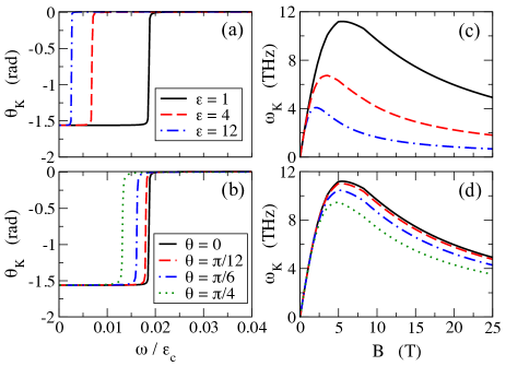
Figure 3: (Color online) Effect of substrate and oblique incidence on the low-frequency Kerr rotation. (a)-(b) illustrate the Kerr angle versus frequency for two cases: (a) normal incidence on a TI film with a dielectric substrate of thickness $d_{\mathrm{s}}=0.5\,\mu\mathrm{m}$: $\epsilon=1$ (a free-standing sample), $\epsilon=4$ (a SiO₂ substrate), $\epsilon=12$ (a Si substrate), and (b) oblique incidence on a free-standing TI film at incidence angle $\theta_{i}=0,\pi/12,\pi/6,\pi/4$. The top and surface densities are $n_{\mathrm{T}}=n_{\mathrm{B}}=3\times 10^{11}\,\mathrm{cm}^{-2}$ and $B=25\,\mathrm{T}$. (c)-(d) show respectively the Kerr frequency as a function of magnetic field corresponding to cases (a) and (b) at the same surface densities. The TI film thickness $d=30\,\mathrm{nm}$.

V.2.2 Thin TI film and Thick Substrate

Above we considered the case when the substrate thickness is small compared with the wavelength. We see that as long as the substrate thickness remains smaller than the wavelength, increasing the thickness only suppresses the Kerr frequency window, but the $\pi/2$ rotation at very small frequencies survives. Experimentally, however, one may have to employ a substrate with supra-wavelength thickness for various reasons; this motivates us to consider the effect of a thicker substrate. When the substrate thickness is increased beyond one wavelength, one can expect that the magnitude of the giant Kerr rotation is suppressed. But that is not the end of the story. Indeed, a logic similar to that employed in Section IV B tells us that when the substrate thickness contains an integer number of half wavelength, the resulting Faraday and Kerr rotations will again be independent of the substrate dielectric properties.

For wavelength short compared with the substrate thickness, but still long compared with the TI film thickness ($k_{\mathrm{TI}}d\ll 1$) and $\omega\ll\Delta$ or $\Omega_{\mathrm{B}}$, we find the following phases for the left- and right-handed ($\lambda=\pm$) circularly polarized transmitted and reflected light for normal incidence

$$\mathrm{arg}\left(E_{\lambda}^{\mathrm{t}}\right)=$$

$$\tan^{-1}\frac{2Z_{\mathrm{s}}^{-1}\cos(k_{\mathrm{s}}d_{\mathrm{s}})\left[\lambda 2\pi\sigma_{xy}^{\mathcal{R}}\cos(k_{0}d_{\mathrm{s}})-\sin(k_{0}d_{\mathrm{s}})\right]+\sin(k_{\mathrm{s}}d_{\mathrm{s}})\left[\left(1+Z_{\mathrm{s}}^{-2}\right)\cos(k_{0}d_{\mathrm{s}})+\lambda 4\pi\sigma_{xy}^{\mathcal{R}}\sin(k_{0}d_{\mathrm{s}})\right]}{2Z_{\mathrm{s}}^{-1}\cos(k_{\mathrm{s}}d_{\mathrm{s}})\left[\lambda 2\pi\sigma_{xy}^{\mathcal{R}}\sin(k_{0}d_{\mathrm{s}})+\cos(k_{0}d_{\mathrm{s}})\right]+\sin(k_{\mathrm{s}}d_{\mathrm{s}})\left[\left(1+Z_{\mathrm{s}}^{-2}\right)\sin(k_{0}d_{\mathrm{s}})-\lambda 4\pi\sigma_{xy}^{\mathcal{R}}\cos(k_{0}d_{\mathrm{s}})\right]},$$ (73)

$$\mathrm{arg}\left(E_{\lambda}^{\mathrm{r}}\right)=-\tan^{-1}\left\{\right.$$ (74)

$$\left.\frac{2\left\{\left(Z_{\mathrm{s}}^{-2}+1\right)\lambda 4\pi\sigma_{xy}^{\mathcal{R}}+\left(Z_{\mathrm{s}}^{-2}-1\right)\left[\lambda 4\pi\sigma_{xy}^{\mathcal{R}}\cos(2k_{\mathrm{s}}d_{\mathrm{s}})+Z_{\mathrm{s}}^{-1}\sin(2k_{\mathrm{s}}d_{\mathrm{s}})\right]\right\}}{\left(Z_{\mathrm{s}}^{-2}+1\right)[Z_{\mathrm{s}}^{-2}-1+\left(4\pi\sigma_{xy}^{\mathcal{R}}\right)^{2}]-\left(Z_{\mathrm{s}}^{-2}-1\right)[Z_{\mathrm{s}}^{-2}+1-\left(4\pi\sigma_{xy}^{\mathcal{R}}\right)^{2}]\cos(2k_{\mathrm{s}}d_{\mathrm{s}})+Z_{\mathrm{s}}^{-1}\left(Z_{\mathrm{s}}^{-2}-1\right)\lambda 8\pi\sigma_{xy}^{\mathcal{R}}\sin(2k_{\mathrm{s}}d_{\mathrm{s}})}\right\},$$

where for notational simplicity we have defined the wave impedance $Z_{\mathrm{s}}=\sqrt{\mu_{\mathrm{s}}/\epsilon_{\mathrm{s}}}$ for the substrate.

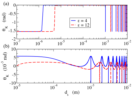
Figure 4: (Color online) (a). Dependence of the low-frequency Kerr rotation of a TI thin film on the substrate thickness $d_{\mathrm{s}}$ for frequency $\omega/\varepsilon_{\mathrm{c}}=10^{-3}$, and substrate dielectric constants $\epsilon=4$ (SiO₂), $\epsilon=12$ (Si). At this frequency, $\lambda\simeq 7\,\mathrm{mm}$ is always much longer than the TI film thickness, but becomes comparable to the substrate thickness when $d_{\mathrm{s}}\sim\lambda/\sqrt{\epsilon_{\mathrm{s}}\mu_{\mathrm{s}}}$. Cavity resonances of the giant Kerr rotation can be seen at values of $d_{\mathrm{s}}$ equal to integer multiples of $\lambda/2\sqrt{\epsilon_{\mathrm{s}}\mu_{\mathrm{s}}}$. (b). Close-up showing the finer features of $\theta_{\mathrm{K}}$ additional to the cavity resonances; Fabry-Perot type oscillations are clearly seen. For thick substrates, the value of $\theta_{\mathrm{K}}$ is strongly suppressed compared to the long-wavelength result away from the cavity resonance values. The values of $n_{\mathrm{T}}$, $n_{\mathrm{B}}$, and $d$ are the same as in Fig. 3.

If, in addition, we impose the requirement that the substrate thickness contains an integer multiple of half wavelengths ($k_{\mathrm{s}}d_{\mathrm{s}}=N\pi$, $N\neq 0$) then Eqs. (73)-(74) greatly simplify, yielding

$$\mathrm{arg}\left(E_{\lambda}^{\mathrm{t}}\right) = \tan^{-1}\frac{\lambda 2\pi\sigma_{xy}^{\mathcal{R}}\cos(k_{0}d_{\mathrm{s}})-\sin(k_{0}d_{\mathrm{s}})}{\lambda 2\pi\sigma_{xy}^{\mathcal{R}}\sin(k_{0}d_{\mathrm{s}})+\cos(k_{0}d_{\mathrm{s}})},$$ (75)

$$\mathrm{arg}\left(E_{\lambda}^{\mathrm{r}}\right) = -\lambda\tan^{-1}\frac{1}{2\pi\sigma_{xy}^{\mathcal{R}}},$$ (76)

from which we recover the quantized Faraday [Eq. (50)] and giant Kerr rotations [Eq. (51)]. This tells us that the Faraday and Kerr rotations can survive suppression effects from a thick substrate as long as the substrate thickness satisfies the resonance condition. Although it is remarkable that Eqs. (50)-(51) still hold in this circumstance, it is important that the light frequency needs to be precisely tuned to the resonant frequency of the substrate. In contrast, if one has the liberty to use a thin substrate, the giant Kerr rotation can be observed in a relatively broad range of frequencies up to $\omega_{\mathrm{K}}$ [Eq. (71)]. Fig. 4 shows the Kerr angle calculated as a function of substrate thickness. We see that the Kerr angle remains $\pi/2$ for substrate thickness $d_{\mathrm{s}}$ much smaller than the wavelength (up to $\sim 1\,\mu\mathrm{m}$ in the plot) and then becomes suppressed for larger substrate thickness. However, when $d_{\mathrm{s}}$ becomes comparable to the wavelength in the substrate, a series of sharply-defined cavity resonance peaks is seen that preserves the giant $\pi/2$ value [Fig. 4 (a)]. Around the same range of $d_{\mathrm{s}}$ values, Fabry-perot like oscillations of the Kerr rotation are also clearly seen in Fig. 4 (b).

VI Generalization to Other Systems with Quantized Hall Conducting Layers

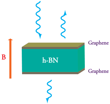
Figure 5: (Color online) Experimental setup of the double-layer graphene heterostructure sandwiching a hexagonal boron nitride (h-BN) substrate. A quantizing magnetic field is applied perpendicularly to the layers.

Because topological insulator properties are at present still obscured by the issue of bulk conduction Transport1 ; Transport2 ; Transport3 ; Transport4 , and because samples do not yet have the quality necessary to yield strongly developed quantum Hall effects, it is natural to ask if similar magneto-optical effects can be achieved in other materials systems. Indeed, the magneto-optical effects we have discussed are not essentially distinct from those of other systems with two nearby conducting layers that exhibit quantum Hall effects. Eqs. (50), (51), (59) for the Faraday and Kerr rotations in Section IV apply to a wide variety of other systems when they are placed in an external magnetic field.

Systems with two nearby graphene layers appear to be particularly attractive because they are also described by massless Dirac equations and, like TI surface states, quite sensitive to time-reversal symmetry breaking perturbations. In fact, the quantum Hall effect can be realized in graphene sheets at magnetic field strengths that are so low QH_Kim1 ; QH_Kim2 ; Geim1 that applications in optics are not out of the question. Aside from integer and fractional quantum Hall effects in external magnetic fields, monolayer and bilayer graphene can also potentially exhibit quantized anomalous Hall effectsGraphene_QAHE1 ; Graphene_QAHE2 ; Franz due to surface adsorption of transition metal atoms.

One experimental system that has now been realized experimentally Kim_BN , but not yet studied optically, consists of two graphene layers separated by a few layers of hexagonal boron nitride. Transport experiments have demonstrated that the quantum Hall effect is already strong in this type of system at fields well below $1$ Tesla. We propose the experimental setup shown in Fig. 5 to observe the dramatic magneto-optical effects. Because of valley and approximate spin degeneracies the strongest quantum Hall effects occur at filling factor $\nu_{\mathrm{T,B}}=\pm 2$, rather than at $\nu_{\mathrm{T,B}}=\pm 1/2$, but this only changes some details of the magneto-optical properties. Indeed, the change in filling factors might be desirable for some potential applications. Realizing systems with two (or indeed many) essentially decoupled layers separated by much less than a wavelength is feasible. The small spacing between essentially isolated quantum Hall layers increases the frequency window over which strong magneto-optical effects are anticipated. In addition bulk conduction is automatically eliminated.

VII Conclusion

We have presented a comprehensive theory for the magneto-optical Faraday and Kerr effects of topological insulator films, and more generally of layered quantized Hall systems. We identify a topological regime in which the light frequency is low compared to surface gaps opened up by time-reversal symmetry breaking perturbations and the light wavelength is either long compared to the film thickness or an integer multiple of twice the film thickness. In the topological regime, the magneto-optical effects are dramatic and universal. For thin films, the Faraday rotation angle is quantized in units of the fine structure constant, and the Kerr angle exhibits a giant $90$ degrees rotation. For thick films that contain a commensurate number of half wavelength, both the Faraday and Kerr rotations are quantized in units of the fine structure constant. In the presence of bulk conduction, the dramatic Faraday and Kerr effects for thin films remain robust as long as the effective two-dimensional conductivity from the bulk, in $e^{2}/h$ units, is smaller than the fine structure constant. The effect of a thick substrate, which may sometimes be experimentally necessary, can be nullified either by making it thinner than a light wavelength or, if it must be thick, by tuning its thickness to an integer number of half wavelength. The giant Kerr effect remains unaffected by oblique incidence when a thin film with a thin substrate is used. These magneto-optical effects can also be realized, perhaps even more readily, in systems with two graphene layers separated by hexagonal boron nitride or another thin dielectric.

VIII Acknowledgement

This work was supported by the Welch under Grant No. F1473 and by DOE under Grant No. DE-FG03-02ER45985. We are indebted to many for their useful discussions throughout the progress of this work: N. Peter Armitage, Kenneth Burch, Dennis Drew, Jim Erskine, Zhong Fang, Jun Kono, Joel Moore, Xiao-Liang Qi, Gennady Shvets, Rolando Valdés Aguilar, David Vanderbilt, and Shou-Cheng Zhang.

IX Appendix. Transmission and Reflection Coefficients at Oblique Incidence

We denote the incident and emergent angles of the electromagnetic wave after scattering with the interface by $\theta_{i}$ and $\theta_{j}$. The matrix elements of the reflection and transmission tensors can be found as

$$r_{xx} = \frac{e^{i2k_{i}a_{i}\cos\theta_{i}}}{D_{ji}}\left\{\sqrt{\frac{\epsilon_{i}}{\mu_{i}}}\cos^{2}\theta_{i}\sec\theta_{j}\left(4\pi{\sigma}_{xx}+\sqrt{\frac{\epsilon_{j}}{\mu_{j}}}\sec\theta_{j}\right)-\sqrt{\frac{\epsilon_{i}}{\mu_{i}}}\left(\sqrt{\frac{\epsilon_{j}}{\mu_{j}}}+4\pi{\sigma}_{xx}\sec\theta_{j}\right)\right.$$

$$\left.-\cos\theta_{i}\left\{4\pi\sqrt{\frac{\epsilon_{j}}{\mu_{j}}}{\sigma}_{xx}+\sec\theta_{j}\left[-\frac{\epsilon_{i}}{\mu_{i}}+\frac{\epsilon_{j}}{\mu_{j}}+16\pi^{2}\left({\sigma}_{xx}^{2}+{\sigma}_{xy}^{2}\right)+4\pi\sqrt{\frac{\epsilon_{j}}{\mu_{j}}}{\sigma}_{xx}\sec\theta_{j}\right]\right\}\right\},$$

$$r_{yy} = -\frac{e^{i2k_{i}a_{i}\cos\theta_{i}}}{D_{ji}}\left\{\sqrt{\frac{\epsilon_{i}}{\mu_{i}}}\cos^{2}\theta_{i}\sec\theta_{j}\left(4\pi{\sigma}_{xx}+\sqrt{\frac{\epsilon_{j}}{\mu_{j}}}\sec\theta_{j}\right)-\sqrt{\frac{\epsilon_{i}}{\mu_{i}}}\left(\sqrt{\frac{\epsilon_{j}}{\mu_{j}}}+4\pi{\sigma}_{xx}\sec\theta_{j}\right)\right.$$

$$\left.+\cos\theta_{i}\left\{4\pi\sqrt{\frac{\epsilon_{j}}{\mu_{j}}}{\sigma}_{xx}+\sec\theta_{j}\left[-\frac{\epsilon_{i}}{\mu_{i}}+\frac{\epsilon_{j}}{\mu_{j}}+16\pi^{2}\left({\sigma}_{xx}^{2}+{\sigma}_{xy}^{2}\right)+4\pi\sqrt{\frac{\epsilon_{j}}{\mu_{j}}}{\sigma}_{xx}\sec\theta_{j}\right]\right\}\right\},$$

$$r_{xy} = -\frac{e^{i2k_{i}a_{i}\cos\theta_{i}}}{D_{ji}}8\pi\sqrt{\frac{\epsilon_{i}}{\mu_{i}}}{\sigma}_{xy}\cos\theta_{i}\sec\theta_{j},$$ (77)

$$t_{xx} = \frac{e^{i\left(k_{i}\cos\theta_{i}-k_{j}\cos\theta_{j}\right)a_{i}}}{D_{ji}}2\sqrt{\frac{\epsilon_{i}}{\mu_{i}}}\cos\theta_{i}\sec\theta_{j}\left[\sqrt{\frac{\epsilon_{i}}{\mu_{i}}}+\cos\theta_{i}\left(4\pi{\sigma}_{xx}+\sqrt{\frac{\epsilon_{j}}{\mu_{j}}}\sec\theta_{j}\right)\right],$$

$$t_{yy} = \frac{e^{i\left(k_{i}\cos\theta_{i}-k_{j}\cos\theta_{j}\right)a_{i}}}{D_{ji}}2\sqrt{\frac{\epsilon_{i}}{\mu_{i}}}\cos\theta_{i}\sec\theta_{j}\left[\sqrt{\frac{\epsilon_{j}}{\mu_{j}}}+\sec\theta_{j}\left(4\pi{\sigma}_{xx}+\sqrt{\frac{\epsilon_{i}}{\mu_{i}}}\cos\theta_{i}\right)\right],$$

$$t_{xy} = -\frac{e^{i\left(k_{i}\cos\theta_{i}-k_{j}\cos\theta_{j}\right)a_{i}}}{D_{ji}}8\pi\sqrt{\frac{\epsilon_{i}}{\mu_{i}}}\cos\theta_{i}\sec\theta_{j}{\sigma}_{xy},$$ (78)

$$r^{\prime}_{xx} = \frac{e^{-i2k_{j}a_{i}\cos\theta_{j}}}{D_{ji}}\left\{-\sqrt{\frac{\epsilon_{i}}{\mu_{i}}}\cos^{2}\theta_{i}\sec\theta_{j}\left(4\pi{\sigma}_{xx}+\sqrt{\frac{\epsilon_{j}}{\mu_{j}}}\sec\theta_{j}\right)+\sqrt{\frac{\epsilon_{i}}{\mu_{i}}}\left(\sqrt{\frac{\epsilon_{j}}{\mu_{j}}}-4\pi{\sigma}_{xx}\sec\theta_{j}\right)\right.$$

$$\left.-\cos\theta_{i}\left\{-4\pi\sqrt{\frac{\epsilon_{j}}{\mu_{j}}}{\sigma}_{xx}+\sec\theta_{j}\left[\frac{\epsilon_{i}}{\mu_{i}}-\frac{\epsilon_{j}}{\mu_{j}}+16\pi^{2}\left({\sigma}_{xx}^{2}+{\sigma}_{xy}^{2}\right)+4\pi\sqrt{\frac{\epsilon_{j}}{\mu_{j}}}{\sigma}_{xx}\sec\theta_{j}\right]\right\}\right\},$$

$$r^{\prime}_{yy} = \frac{e^{-i2k_{j}a_{i}\cos\theta_{j}}}{D_{ji}}\left\{-\sqrt{\frac{\epsilon_{i}}{\mu_{i}}}\cos^{2}\theta_{i}\sec\theta_{j}\left(4\pi{\sigma}_{xx}-\sqrt{\frac{\epsilon_{j}}{\mu_{j}}}\sec\theta_{j}\right)-\sqrt{\frac{\epsilon_{i}}{\mu_{i}}}\left(\sqrt{\frac{\epsilon_{j}}{\mu_{j}}}+4\pi{\sigma}_{xx}\sec\theta_{j}\right)\right.$$

$$\left.-\cos\theta_{i}\left\{4\pi\sqrt{\frac{\epsilon_{j}}{\mu_{j}}}{\sigma}_{xx}+\sec\theta_{j}\left[\frac{\epsilon_{i}}{\mu_{i}}-\frac{\epsilon_{j}}{\mu_{j}}+16\pi^{2}\left({\sigma}_{xx}^{2}+{\sigma}_{xy}^{2}\right)-4\pi\sqrt{\frac{\epsilon_{j}}{\mu_{j}}}{\sigma}_{xx}\sec\theta_{j}\right]\right\}\right\},$$

$$r^{\prime}_{xy} = -\frac{e^{-i2k_{j}a_{i}\cos\theta_{j}}}{D_{ji}}8\pi\sqrt{\frac{\epsilon_{j}}{\mu_{j}}}{\sigma}_{xy}\cos\theta_{i}\sec\theta_{j},$$ (79)

$$t^{\prime}_{xx} = \frac{e^{i\left(k_{i}\cos\theta_{i}-k_{j}\cos\theta_{j}\right)a_{i}}}{D_{ji}}2\sqrt{\frac{\epsilon_{j}}{\mu_{j}}}\left[\sqrt{\frac{\epsilon_{i}}{\mu_{i}}}+\cos\theta_{i}\left(4\pi{\sigma}_{xx}+\sqrt{\frac{\epsilon_{j}}{\mu_{j}}}\sec\theta_{j}\right)\right],$$

$$t^{\prime}_{yy} = \frac{e^{i\left(k_{i}\cos\theta_{i}-k_{j}\cos\theta_{j}\right)a_{i}}}{D_{ji}}2\sqrt{\frac{\epsilon_{j}}{\mu_{j}}}\left[\sqrt{\frac{\epsilon_{j}}{\mu_{j}}}+\sec\theta_{j}\left(4\pi{\sigma}_{xx}+\sqrt{\frac{\epsilon_{i}}{\mu_{i}}}\cos\theta_{i}\right)\right],$$

$$t^{\prime}_{xy} = -\frac{e^{i\left(k_{i}\cos\theta_{i}-k_{j}\cos\theta_{j}\right)a_{i}}}{D_{ji}}8\pi\sqrt{\frac{\epsilon_{j}}{\mu_{j}}}\cos\theta_{i}\sec\theta_{j}{\sigma}_{xy},$$ (80)

where

$$D_{ji} = \sqrt{\frac{\epsilon_{i}}{\mu_{i}}}\cos^{2}\theta_{i}\sec\theta_{j}\left(4\pi{\sigma}_{xx}+\sqrt{\frac{\epsilon_{j}}{\mu_{j}}}\sec\theta_{j}\right)+\sqrt{\frac{\epsilon_{i}}{\mu_{i}}}\left(\sqrt{\frac{\epsilon_{j}}{\mu_{j}}}+4\pi{\sigma}_{xx}\sec\theta_{j}\right)$$ (81)

$$+\cos\theta_{i}\left\{4\pi\sqrt{\frac{\epsilon_{j}}{\mu_{j}}}{\sigma}_{xx}+\sec\theta_{j}\left[\frac{\epsilon_{i}}{\mu_{i}}+\frac{\epsilon_{j}}{\mu_{j}}+16\pi^{2}\left({\sigma}_{xx}^{2}+{\sigma}_{xy}^{2}\right)+4\pi\sqrt{\frac{\epsilon_{j}}{\mu_{j}}}{\sigma}_{xx}\sec\theta_{j}\right]\right\}.$$

Note that $r_{yy},t_{yy}$ are no longer equal to $r_{xx},t_{xx}$ at oblique light incidence. Eqs. (78)-(81) recover the normal incidence results Eqs. (35)-(41) when $\theta_{i}=\theta_{j}=0$.

For completeness, we also include the expressions of the total reflection and transmission tensors in the presence of a layer of dielectric substrate. These can be composed from the expressions Eqs. (42)-(43):

$$\bar{r} = \bar{r_{\mathrm{T}}}+\bar{t_{\mathrm{T}}^{\prime}}\bar{r_{\mathrm{S,B}}}\left(\bm{1}-\bar{r_{\mathrm{T}}^{\prime}}\bar{r_{\mathrm{S,B}}}\right)^{-1}\bar{t_{\mathrm{T}}},$$ (82)

$$\bar{t} = \bar{t_{\mathrm{S,B}}}\left(\bm{1}-\bar{r_{\mathrm{T}}^{\prime}}\bar{r_{\mathrm{S,B}}}\right)^{-1}\bar{t_{\mathrm{T}}}.$$ (83)

where $\bar{r_{\mathrm{S,B}}^{(^{\prime})}}$ and $\bar{t_{\mathrm{S,B}}^{(^{\prime})}}$ (the subscript ’S’ denotes substrate) are the reflection and transmission tensors for light propagation from the bottom surface to the substrate-vacuum interface

$$\bar{r_{\mathrm{S,B}}} = \bar{r_{\mathrm{B}}}+\bar{t_{\mathrm{B}}^{\prime}}\bar{r_{\mathrm{S}}}\left(\bm{1}-\bar{r_{\mathrm{B}}^{\prime}}\bar{r_{\mathrm{S}}}\right)^{-1}\bar{t_{\mathrm{B}}},$$ (84)

$$\bar{t_{\mathrm{S,B}}} = \bar{t_{\mathrm{S}}}\left(\bm{1}-\bar{r_{\mathrm{B}}^{\prime}}\bar{r_{\mathrm{S}}}\right)^{-1}\bar{t_{\mathrm{B}}},$$ (85)

where $\bar{r_{\mathrm{S}}^{(^{\prime})}}$ and $\bar{t_{\mathrm{S}}^{(^{\prime})}}$ are the reflection and transmission tensors for light scattering at the substrate-vacuum interface.

References

- (1) L. Fu, C. L. Kane, and E. J. Mele, Phys. Rev. Lett. 98, 106803 (2007).
- (2) J. E. Moore and L. Balents, Phys. Rev. B 75, 121306(R) (2007).
- (3) R. Roy, Phys. Rev. B 79, 195321 (2009).
- (4) For recent reviews, see M. Z. Hasan and C. L. Kane, Rev. Mod. Phys. 82, 3045 (2010); X.-L. Qi and S.-C. Zhang, arXiv:1008.2026v1.
- (5) A. B. Sushkov, G. S. Jenkins, D. C. Schmadel, N. P. Butch, J. Paglione, and H. D. Drew, Phys. Rev. B 82, 125110 (2010); G. S. Jenkins, A. B. Sushkov, D. C. Schmadel, N. P. Butch, P. Syers, J. Paglione, and H. D. Drew, Phys. Rev. B 82, 125120 (2010).
- (6) R. Valdés Aguilar, A. V. Stier, W. Liu, L. S. Bilbro, D. K. George, N. Bansal, J. Cerne, A. G. Markelz, S. Oh, and N. P. Armitage, arXiv:1105.0237v2.
- (7) J. N. Hancock, J. L. M. van Mechelen, A. B. Kuzmenko, D. van der Marel, C. Brune, E. G. Novik, G. V. Astakhov, H. Buhmann, L. Molenkamp, arXiv:1105.0884v1.
- (8) X.-L. Qi, T. L. Hughes, and S.-C. Zhang, Phys. Rev. B 78, 195424 (2008).
- (9) A. M. Essin, J. E. Moore, and D. Vanderbilt, Phys. Rev. Lett. 102, 146805 (2009).
- (10) W.-K. Tse and A. H. MacDonald, Phys. Rev. Lett. 105, 057401 (2010).
- (11) W.-K. Tse and A. H. MacDonald, Phys. Rev. B 82, 161104(R) (2010).
- (12) M. Z. Hasan, Physics 3, 62 (2010).
- (13) J. Maciejko, X.-L. Qi, H. D. Drew, and S.-C. Zhang, Phys. Rev. Lett. 105, 166803 (2010).
- (14) G. Tkachov and E. M. Hankiewicz, Phys. Rev. B 84, 035405 (2011).
- (15) F. Wilczek, Phys. Rev. Lett. 58, 1799 (1987).
- (16) F. D. M. Haldane, Phys. Rev. Lett. 61, 2015 (1988).
- (17) C. L. Kane and E. J. Mele, Phys. Rev. Lett. 95, 226801 (2005).
- (18) Y. Xia, L. Wray, D. Qian, D. Hsieh, A. Pal, H. Lin, A. Bansil, D. Grauer, Y. S. Hor, R. J. Cava, and M. Z. Hasan, arXiv:0812.2078v1 (2008).
- (19) L. A. Wray, S.-Y. Xu, Y. Xia, D. Hsieh, A. V. Fedorov, H. Lin, A. Bansil, Y. S. Hor, R. J. Cava, and M. Z. Hasan, Nature Physics 7, 32 (2011).
- (20) Y. L. Chen, J. H. Chu, J. G. Analytis, Z. K. Liu, K. Igarashi, H. H. Kuo, X.-L. Qi, S. K. Mo, R. G. Moore, D. H. Lu, M. Hashimoto, T. Sasagawa, S.-C. Zhang, I. R. Fisher, Z. Hussain, and Z. X. Shen, Science 329, 659 (2010).
- (21) J. J. Cha, J. R. Williams, D. Kong, S. Meister, H. Peng, A. J. Bestwick, P. Gallagher, D. Goldhaber-Gordon, and Y. Cui, Nano Lett. 10, 1076 (2010).
- (22) D. Hsieh, Y. Xia, D. Qian, L. Wray, J. H. Dil, F. Meier, J.Osterwalder, L. Patthey, J. G. Checkelsky, N. P. Ong, A. V. Fedorov, H. Lin, A. Bansil, D. Grauer, Y. S. Hor, R. J. Cava, and M. Z. Hasan, Nature 460, 1101 (2009).
- (23) P. Cheng, C. Song, T. Zhang, Y. Zhang, Y. Wang, J.-F. Jia, J. Wang, Y. Wang, B.-F. Zhu, X. Chen, X. Ma, K. He, L. Wang, X. Dai, Z. Fang, X. C. Xie, X.-L. Qi, C.-X. Liu, S.-C. Zhang, Q.-K. Xue, Phys. Rev. Lett. 105, 076801 (2010).
- (24) T. Hanaguri, K. Igarashi, M. Kawamura, H. Takagi, and T. Sasagawa, Phys. Rev. B 82, 081305 (2010).
- (25) In Ref. [QiBulkSubstrate, ], the Kerr angle result Eq. (2) is not correct outside of the long-wavelength limit, since is not an integer multiple of when is. The result applies correctly in the long-wavelength limit only with an infinitely thick substrate.
- (26) V. A. Kulbachinskii, N. Miura, H. Nakagawa, H. Arimoto, T. Ikaida, P. Lostak, and C. Drasar, Phys. Rev. B. 59, 15733 (1999).
- (27) A. D. LaForge, A. Frenzel, B. C. Pursley, T. Lin, X. Liu, J. Shi, and D. N. Basov, Phys. Rev. B 81, 125120 (2010).
- (28) N. P. Butch, K. Kirshenbaum, P. Syers, A. B. Sushkov, G. S. Jenkins, H. D. Drew, and J. Paglione, Phys. Rev. B 81, 241301(R) (2010).
- (29) J. G. Analytis, J.-H. Chu, Y. Chen, F. Corredor, R. D. McDonald, Z. X. Shen, and I. R. Fisher, Phys. Rev. B 81, 205407 (2010); J. G. Analytis, R. D. McDonald, S. C. Riggs, J.-H. Chu, G. S. Boebinger, and I.R. Fisher, Nat. Phys. 6, 960 (2010).
- (30) N. Bansal, Y. S. Kim, M. Brahlek, E. Edrey, S. Oh, arXiv:1104.5709v1.
- (31) K. Eto, Z. Ren, A. A. Taskin, K. Segawa, and Yoichi Ando, Phys. Rev. B 81, 195309 (2010).
- (32) N. P. Butch, K. Kirshenbaum, P. Syers, A. B. Sushkov, G. S. Jenkins, H. D. Drew, and J. Paglione, Phys. Rev. B 81, 241301(R) (2010).
- (33) K. I. Bolotin, F. Ghahari, M. D. Shulman, H. L. Stormer, and P. Kim, Nature 462, 196 (2009).
- (34) F. Ghahari, Y. Zhao, P. Cadden-Zimansky, K. I. Bolotin, and P. Kim, Phys. Rev. Lett. 106, 046801 (2011).
- (35) A. S. Mayorov, D. C. Elias, M. Mucha-Kruczynski, R. V. Gorbachev, T. Tudorovskiy, A. Zhukov, S. V. Morozov, M. I. Katsnelson, V. I. Fal’ko, A. K. Geim, and K. S. Novoselov, arXiv:1108.1742v1 (2011).
- (36) W.-K. Tse, Z. Qiao, Y. Yao, A. H. MacDonald, and Q. Niu, Phys. Rev. B 83, 155447 (2011).
- (37) Z. Qiao, S. A. Yang, W. Feng, W.-K. Tse, J. Ding, Y. Yao, J. Wang, and Q. Niu, Phys. Rev. B 82, 161414 (2010).
- (38) C. Weeks, J. Hu, J. Alicea, M. Franz, and R. Wu, arXiv:1104.3282v1 (2011).
- (39) C. R. Dean, A. F. Young, I. Meric, C. Lee, L. Wang, S. Sorgenfrei, K. Watanabe, T. Taniguchi, P. Kim, K. L. Shepard, and J. Hone, Nat. Nanotech. 5, 722 (2010).