Spontaneous Polaron Transport in Biopolymers

Abstract

Polarons, introduced by Davydov to explain energy transport in $\alpha$-helices, correspond to electrons localised on a few lattice sites because of their interaction with phonons. While the static polaron field configurations have been extensively studied, their displacement is more difficult to explain. In this paper we show that, when the next to nearest neighbour interactions are included, for physical values of the parameters, polarons can spontaneously move, at $T=0$, on bent chains that exhibit a positive gradient in their curvature. At room temperature polarons perform a random walk but a curvature gradient can induce a non-zero average speed similar to the one observed at zero temperature. We also show that at zero temperature a polaron bounces on sharply kinked junctions. We interpret these results in light of the energy transport by transmembrane proteins.

1 Introduction

Proteins, essential components of all biological cells are central to their proper functioning. As “form determines function”, a study of protein structure and dynamics is of utmost importance in elucidating their role in cellular behaviour. One of the key problems in biology is to understand energy transport from one part of the cell to another and to study the role of protein conformations and conformational transitions in this process.

The mechanism of charge and energy transport in proteins and other bio-macromolecules at the atomic scale was proposed Davydov and co-workers[1]. In this approach the transport properties are considered in terms of the emergence of a ‘polaron’ whose properties and dynamics are used to describe the resultant transport. The polaron describes a localised excitation which carries energy corresponding to some vibrational modes of a group of molecules and a distortion of the chain containing these molecules. The system acts as a particle and its dynamical properties can be studied in terms of solutions of particular differential equations that describe its behaviour.

The Davydov theory hinges on the assumption that an extra electron or energy quanta released in the hydrolysis of ATP (adenosine triphosphate) can be stored by the protein molecule in its vibrational mode. The non-linear coupling between the vibrational mode and other excitations on the chain leads to the formation of a soliton (polaron in the case of the interaction between the phonon modes and the electron in a polarizable medium). The soliton (polaron in this case) can then propagate along the polypeptide backbone leading to energy/charge transport. The soliton mediated transport mechanism has been applied to helical proteins[2]. The theory of non-linear energy transport in bio-molecules is reviewed in [3, 4]. Most of the studies are based on simple models of one-dimensional reductions of the three-dimensional structure of the $\alpha$-helix proteins i.e., only a single strand of hydrogen-bonded peptide units is considered. Moreover, the original set of discrete lattice equations is often treated in a continuum approximation. Recent studies based on two and three-dimensional models describing the solitonic and/or polaronic transport of energy are described in detail in [5, 6, 7, 8].

Studies of polaron transport on $\alpha$ helical polymers have recently been reported by Henning [9]. The Henning model is an extension of semiclassical treatments of polaron transport within the Holstein model which incorporates three strands that comprise the $\alpha$ helix. Numerical schemes and variational approaches have been utilized in the treatments of the Holstein model with a hard non-linear on-site potential term in one dimension to obtain polaronic ground states, their phase diagram in terms of the non-linearity parameter as well as the one characterising the electron-phonon coupling[10, 11, 12]. It has also been shown that the presence of the non-linear on-site potential polaron formation is possible in higher dimensions, a fact borne out by the Henning model. Normal mode analysis of this model revealed the existence of a low-frequency pinning mode, and hence enabled the construction of one and two-dimensional moving polaron solutions by a Floquet analysis[10, 11]. The effects of the lattice non-linearity were reported to have led to a dramatic reduction of the polaron effective mass.

However, in most of these studies the polaron is “kicked” from its rest state via a perturbation[13]. In this paper we look at the spontaneous polaron transport via charge-conformational coupling. In particular, we study polaron transport on a flexible chain with an imposed initial bend at both zero ($T=0$) and non-zero ($T\neq 0$) temperatures. We now summarise our main results.

At $T=0$ a polaron can undergo spontaneous motion via the coupling of charge with the conformational degrees of freedom. Thus an imposed bend on the chain causes the polaron to accelerate. However, we have found that when such an accelerating polaron encounters a kink, a slope discontinuity along the chain backbone, it gets reflected instead of continuing along its original direction of motion guided by inertia. The reason for this due to the long-range nature of the exchange coupling term. At finite temperature $T\neq 0$ thermal fluctuations wash away directed transport and the polaron undergoes large amplitude fluctuations about its mean position. However, since the chain ends act as reflecting walls, a polaron formed closer to one end of a straight chain would often get reflected, resulting in an overall small but non-negligible drift.

The paper is organised as follows: In the next section we present the Hamiltonian describing polaron transport on a flexible chain and change variables to dimensionless quantities. The dimensionless parameter values corresponding to physically relevant systems e.g. proteins are computed in Sec.3. We describe the results of our numerical studies in Sec.4 and we set our work in perspective in the final section.

2 Polaron Hamiltonian on a Flexible Chain

We consider a modified version of the polaron model proposed by Mingaleev et al.[14]. Our model involves a semi-classical treatment of the interaction between a phonon field ${\vec{R}_{n}}$ and an electron field $\phi_{n}$ on a flexible linear chain whose nodes are labelled by an index $n$.

The Hamiltonian of the model is given by

$$H = \sum_{n}\left[\frac{\hat{M}}{2}\left(\frac{d{\vec{R}_{n}}}{d\tau}\right)^{2}+\hat{U}_{n}({\vec{R}})+W\left(2|{\phi_{n}}|^{2}-\sum_{m\neq n}J_{nm}\phi_{n}^{*}\phi_{m}\right)-\frac{1}{2}\Delta|\phi_{n}|^{4}\right],$$ (1)

where $M$ is the mass of the chain node, $W$ is the linear excitation transfer energy and $\Delta$ the non-linear self-trapping interaction. The excitation transfer coefficients $J_{n,m}$ are of the form:

$$J_{n,m}=J(|{\vec{r}_{n}}-{\vec{r}_{m}}|)=(e^{\alpha}-1)\,e^{-\alpha|{\vec{r}_{n}}-{\vec{r}_{m}}|/a},$$ (2)

where $\alpha^{-1}$ sets the relative length scale over which the interaction decreases, in units of $a$, and where $a$ is the rest distance between two adjacent sites. The $J_{n,m}$ describes the long range interaction between the electron field at different lattice sites $n$ and $m$; its value decreases exponentially with the distance between them.

Note that the normalisation of the electron field is preserved in our model, i.e.

$$\sum_{n}|\phi_{n}|^{2}=1.$$ (3)

The phonon potential $U_{n}$ consists of three terms:

$$\hat{U}_{n}({\vec{R}})=\frac{\hat{\sigma}}{2}(|{\vec{R}_{n}}-{\vec{R}_{n-1}}|-\hat{a})^{2}+\frac{\hat{k}}{2}\frac{(\theta_{n}-\varphi_{n})^{2}}{\left[1-((\theta_{n}-\varphi_{n})/\theta_{max})^{2}\right]}$$

$$+\frac{\hat{\delta}}{2}\sum_{m\neq n}(\hat{d}-|{\vec{R}_{n}}-{\vec{R}_{m}}|)^{2}\Theta(\hat{d}-|{\vec{R}_{n}}-{\vec{R}_{m}}|).$$ (4)

The first term in Eq.(4) models the elastic energy describing the stretching of the adjacent nodes of the chain, where $\hat{a}$ is the equilibrium separation between them. The second term describes the bending energy of the chain akin to semi-flexible polymers. Here $\varphi_{n}$ is the rest angle between adjacent lattice links and $\theta_{max}$ is the largest angle allowed. In the Mingaleev model[14] $\varphi_{n}=0$ and the equilibrium configuration of the chain is a straight one. Non-zero values of $\varphi_{n}$ lead to a bent chain. The last term, (proportional to $\hat{\delta}$), models hard-core repulsion between the atoms of the chain. However, we note that this term does not contribute significantly in determining the equilibrium chain conformation.

In this paper symbols denoted by an overhead carat sign e.g. $\hat{M}$, $\hat{\sigma}$ etc. correspond to physical variables carrying units and dimensions while those without it correspond to non-dimensional variables and parameters. We rescale time $\tau$ by defining a timescale $\tau_{0}=\frac{\hbar\Delta}{W^{2}}$s and rescale distances by a length scale $a$. The non-linear coupling parameter $g$ appears as a dimensionless ratio of two energy scales.

$$\tau = t\tau_{0}\qquad\qquad g=\frac{\Delta}{W}\qquad\qquad r=\frac{R}{a}.$$ (5)

In terms of these variables the Hamiltonian takes the form

$$H = \frac{W^{2}}{\Delta}\sum_{n}\left[\frac{M}{2}\left(\frac{d{\vec{r}_{n}}}{dt}\right)^{2}+U_{n}({\vec{r}})+g\left(2|{\phi_{n}}|^{2}-\sum_{m\neq n}J_{nm}\phi_{n}^{*}\phi_{m}\right)-\frac{g^{2}}{2}|\phi_{n}|^{4}\right],$$ (6)

where

$$U_{n}({\vec{r}})=\frac{\sigma}{2}(|{\vec{r}_{n}}-{\vec{r}_{n-1}}|-a)^{2}+\frac{k}{2}\frac{(\theta_{n}-\varphi_{n})^{2}}{\left[1-((\theta_{n}-\varphi_{n})/\theta_{max})^{2}\right]}+\frac{\delta}{2}\sum_{m\neq n}(d-|{\vec{r}_{n}}-{\vec{r}_{m}}|)^{2}\Theta(d-|{\vec{r}_{n}}-{\vec{r}_{m}}|)$$ (7)

with

$$M = \hat{M}\frac{a^{2}W^{2}}{\hbar^{2}\Delta}\qquad\qquad\sigma=\hat{\sigma}\frac{a^{2}\Delta}{W^{2}}\qquad\qquad\delta=\hat{\delta}\frac{a^{2}\Delta}{W^{2}}$$

$$k = \hat{k}\frac{\Delta}{W^{2}}\qquad\qquad a=\frac{\hat{a}}{a}=1\qquad\qquad d=\frac{\hat{d}}{a}.$$ (8)

Writing ${\vec{r}_{n}}=(x_{1,n},x_{2,n},x_{3,n},)$ we can derive the equation of motion for $x_{i,n}$ from the Hamiltonian Eq.(6). Thermal fluctuations are incorporated by adding a delta correlated white noise $F(t)$ which satisfies

$$<F(0)F(s)>=2\Gamma k_{B}T\delta(s).$$ (9)

The resulting Langevin equations describing the coupled dynamics of the chain and of the polaron is given by

$$M\frac{d^{2}x_{i,n}}{dt^{2}}+\Gamma\frac{dx_{i,n}}{dt}+F(t)+\sum_{m}\frac{dU_{m}}{dx_{i,n}}-g\sum_{k}\sum_{m<k}\frac{dJ_{km}}{dx_{i,n}}(\phi_{k}^{*}\phi_{m}+\phi_{m}^{*}\phi_{k}) = 0$$

$$i\frac{d\phi_{n}}{dt}-2\phi_{n}+\sum_{m\neq n}J_{nm}\phi_{m}+g|{\phi_{n}}|^{2}\phi_{n} = 0,$$ (10)

Note that we also have

$$\overline{k_{B}T}=k_{B}T\frac{W^{2}}{\Delta}=k_{B}TWg$$ (11)

and, as the equation for $x_{i}$ is expressed in units of $W^{2}/(\Delta a)$, we have $\Gamma=\hat{\Gamma}a^{2}/\hbar$.

3 Physical Parameter Values

In order to study the feasibility of the mechanism of the energy transport via polarons for biologically relevant systems we have used the parameter values corresponding to those of $\alpha$-helices.

We note that for Amid-I vibrations in $\alpha$-helices [15] we have: $W\approx 2\times 10^{-22}J\approx 1.2meV$, $\hat{\sigma}=19.5N/m$ and $\hat{M}=2\times 10^{-25}kg$. $a\approx 0.45nm$. $\epsilon=0.02eV$. $\Delta=8\frac{\epsilon^{2}}{\hat{\sigma}}=4.74\times 10^{-22}J=0.003eV$. Moreover, $\hat{k}$ can be evaluated from the persistence length of $\alpha$-helices $\lambda\approx 65nm$ [16]

$$\hat{k}=\lambda k_{B}T/a\approx 6\times 10^{-19}J.$$ (12)

Though we do not have experimental values of $\hat{\delta}$, it is clear that it must be larger than $\hat{\sigma}$. For the friction coefficient we assume that $\hat{\Gamma}\approx 6\pi\mu a$, where $\mu=0.001Pa\,s$ is the water viscosity. Incidentally, for the cytoplasm $\mu$ is up to $4$ times larger than this value.

At “room” temperature $T=300K$, the non-dimensional parameter values are

$$g=2.5\qquad\qquad \sigma=51351.\qquad\qquad k=7776\qquad\qquad\Gamma=8143$$ (13)

$$M=2.79\times 10^{5}\qquad\qquad k_{B}T=54\qquad\qquad\nu=0.01\qquad\qquad\tau_{0}=10^{-12}s.$$

Following Mingaleev et al. [14] we choose $\alpha=2$.

Next we have performed the simulation of the time evolution described by the equations Eq.(2) - to explore the coupled dynamics of polaron transport and the conformational transitions of the chain associated with such motion. For the values of $g$ and $k$ mentioned above, we have found that the physical $\alpha$-helices are too rigid for the polaron to bend the chain and move along it as suggested for DNA in [14] (see Fig. 2 in [14] where our $g$ corresponds to $N$).

As a matter of fact, physical polarons always have a relatively small energy, too small to bend a polymer spontaneously, even for DNA. Nevertheless, the Mingaleev et al. model can be used to study the properties of polarons on chains that are, like most proteins, naturally bent. One can expect the electron-phonon interaction to lead to the spontaneous displacement of polarons on bending gradients for the following reason: the main effect of the electron-phonon interaction is to favour configurations where the distance between nodes is reduced (i.e. the interatomic separation is smaller than the equilibrium lattice spacing in the vicinity of the polaron). As a kink in the linear chain reduces the distance between nodes that are not adjacent to each other, one expects that the polaron would be attracted by the kink. Thus chain conformations where the angle between consecutive tangent vectors increases monotonically serve as an attractive potential as seen by the polaron. It is thus expected that the polaron will accelerate towards a region of high curvature.

In the next section we present the results of investigations of whether these expectations are correct for the physically relevant proteins (i.e for chains with physically relevant values of their parameters).

4 Polaron on a Bent Chain

We consider a chain of $N=60$ points with a bent mid-section i.e. the region between $n=25$ and $n=45$. Such a configuration is achieved by setting, initially, $\varphi_{n}$ as follows:

$$\begin{array}[]{ll}n<25&\varphi_{n}=0\\ 25\leq n\leq 45&\varphi_{n}=(n-25)d\varphi\\ n>45&\varphi_{n}=0,\\ \end{array}$$ (14)

where $d\varphi$ is the incremental increase in the angle between adjacent links.

In order to numerically simulate the dynamics of the polaron on such a chain, we initially generated and saved the polaron on an undeformed (i.e. straight) lattice ($\varphi_{n}=0$ for all $n$). Such a polaron was obtained by a relaxation method: a friction term was added to the phonon field and the eigenvalue problem for the electron field was solved simultaneously by relaxation. Starting with an electron spread over a few lattice sites and located on a node which we have chosen to be $n=30$, the system was relaxed until both the electron and the phonon fields reached a stationary configuration. This produced a polaron configuration centred at $n=30$. The lattice was then deformed by changing the values of $\varphi_{n}$ to those of (14) and a second relaxation was performed to let the phonon field reach its equilibrium configuration. The electron field of the relaxed polaron was then restored, the time set to $t=0$, and the equations for the phonon and electron fields integrated numerically.

The zero temperature ($T=0$) dynamics was obtained by numerically integrating the electron and phonon fields in Eq.(2) employing a fourth order Runge-Kutta scheme, noting the time it took for the electron to start moving.

Fig. 1 summarises our results for $T=0$. Panel (a) shows typical trajectories of a polaron for different values of $\alpha$, the parameter that models the range of the long-ranged interaction $J_{mn}$ (Eq.(2)) Our simulations show that the main effect of including the next to the nearest neighbour interaction is to make the polaron “to get attracted” to the bend. This is caused by the fact that the lattice points near this bend are nearer to each other and this lowers the energy of the polaron. Hence, on a bent chain, with a slowly increasing bending angle, the polaron is attracted increasingly to the bend as it moves along the chain. This corresponds to the spontaneous displacement of the polaron. It is curious to note that upon reaching the edge of the bent chain beyond which the chain is straight the polaron is reflected. This can be explained by the fact that the energy of the polaron is the lowest where the bending angle is large and the highest where the chain is straight. The transition from a bent to a straight configuration thus corresponds to a potential wall on which the polaron bounces. One notices also that as the parameter $\alpha$ is increased the exchange energy between non adjacent nodes decreases more rapidly with the distance separating them. This results in a smaller acceleration of the polaron as seen in Fig. 1. The speed of the polaron was evaluated as $V=[n(t_{0}+\Delta t)-n(t_{0})]/\Delta t$ where $t_{0}$ is the time at which the polaron started to move and $\Delta t=50$. When the polaron travelled a distance larger than 20, we took $V=20/\Delta t$ where $\Delta t$ was the time taken to cover this distance.

Fig. 1(b) shows the chain configuration with the electron density superimposed on it. Each filled circle (black) corresponds to a lattice point, while the electron density, denoted in grey/yellow, is overlayed on them. The intensity of the lighter circles provides a measure of the electron density at a particular site, i.e. a lighter colour corresponds to a higher electron density. The maximum in the electron density corresponds to the position of the polaron used to generate Fig. 1(a).

\begin{picture}(14.0,7.0)\epsfbox{Fig1a.eps} \epsfbox{Fig1bv2.ps} \end{picture}

Figure 1: Polaron displacement on a bent chain with $d\varphi=0.01$ at $T=0$ for a $N=60$ chain with the initial polaron position at $x_{0}=30$. The time step of integration is chosen to be $dt=50$. Panel (a) shows the trajectory of the polaron on the bent chain for different values of $\alpha$ ($\alpha=1$ (red solid line), $\alpha=1.5$ (blue dashed line), $\alpha=2$ (green dash-dotted line), and $\alpha=2.2$ (magenta dotted line). Panel (b) shows the chain configuration and the electron density. Each circle corresponds to a node and a lighter colour corresponds to a higher electron density.

Next we have investigated the dependence of the polaron dynamics on $d\varphi$ - the gradient of the bending angle of the chain. Fig. 2 shows the variation of the average velocity $\langle V\rangle$ as a function of $d\varphi$. For our choice of parameter values the polaron does not move until a critical value $d\varphi\approx 0.0056$ is reached. The dependence of the velocity on $d\varphi$ in the critical region follows a power law $\langle V\rangle\sim\left(d\varphi-d\varphi_{c}\right)^{\nu}$ akin to elastic depinning of interfaces. In order to express the average speed in physical units, we have to multiply the dimensionless speed by $a/t\approx 328.5\frac{nm}{ns}$. Thus the average speed of the polaron $\langle V\rangle\approx 16nm/ns$.

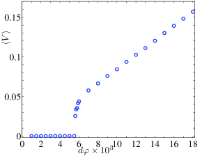
Figure 2: Figure showing the variation of the velocity $\langle V\rangle$ as a function of the bend angle $d\varphi$ for a bent chain of $N=60$ nodes. The initial position of the polaron is at $x_{0}=30$, the bent region extends from $n=25$ to $n=45$ and $T=0$. The speed was computed as $V=d/\Delta t$ where $\Delta t=50$ and $d$ is the distance travelled by the polaron during this time interval.

In order to study the effect of thermal fluctuations on the polaron transport we have performed finite temperature $T\neq 0$ simulations. For such simulations we generated a polaron on a straight lattice at $T=0$ as above and saved it. Next, we deformed the lattice into a bent configuration as above and integrated our equations for $300$ units of time to ensure thermal equilibrium. We then restored the electron field, without altering the phonon field, and numerically integrated Eq (2) with the noise term to investigate the motion of the polaron along the chain. This simulation strategy, faithfully mimics the sudden excitation of a polaron and its time evolution.

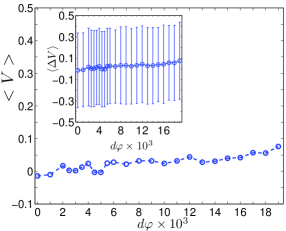
Figure 3: Figure shows the variation of the average velocity $\langle V\rangle$ as a function of the bend angle $d\varphi$ for a $N=60$ chain. The chain is bent between $n=[25,45]$ nodes, and the initial position of the polaron is at $x_{0}=30$. The temperature $T=300K$, and the data is averaged over $N_{run}=1000$ simulations. The speed was evaluated exactly like in figure 2. Inset shows the variance of the velocity vs. $d\varphi$ data.

Our finite temperature studies have focused on the polaron dynamics at “room temperature”, i.e. $T=300K$. Clearly, the effects of taking non-zero temperature are very significant as seen in Fig. 3. It is clear from this figure that the polaron undergoes large amplitude fluctuations about its initial position and its velocity is significantly altered by the thermal effects. The thermally averaged polaron velocity shown in Fig. 3 is averaged over $N_{run}=1000$ simulations, each time having measured the average displacement over $t=50$ units of time. In all cases the life time of the polaron was of the order $t=200$, in our units, which corresponds to about $300ps$. Afterwards the electron was delocalised on the lattice. In Fig. 4 we have plotted the variation of the thermally averaged velocity as a function of $d\varphi$; this is to be compared with the curve obtained for $T=0$ in Fig. 2.

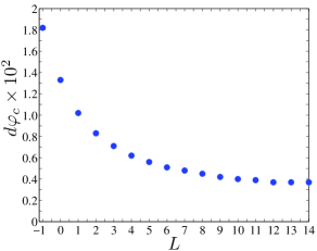
Figure 4: Figure shows the variation of the critical bend angle $d\varphi_{c}$ as a function of the initial relative polaron position L with respect to the bent region, $n_{0,pol}=25+L$. N = 60 and T = 0. The speed was evaluated exactly like in figure 2.

Our simulations clearly show that the thermal effects lead to a wider displacement of the polaron wich can involve motion in both directions. The polaron is thus subjected to a random walk motion in a system with an attractive force provided by the bend of the chain. So, while the displacement of a polaron in a protein at room temperature is random, its position is still biased by the bending gradient; a thermalised polaron thus follows a random walk, but its average displacement is similar to that of a polaron at $T=0$.

In order to quantify the dependence of the bend on the spontaneous transport of polarons we have calculated the dependence of the critical incremental angle between segments $d\varphi_{c}$ on its initial distance from the bend at $T=0$. This is shown in Fig. 4. It is clear from the plot that $d\varphi_{c}\propto\exp[-\xi L]$, where $\xi$ is a constant and L is the distance between the polaron and the edge of the region with the bend.

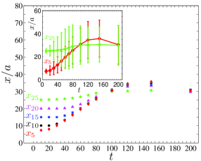
Figure 5: Figure shows the average position of a polaron as a function of time for a straight chain of $N=60$ segments at $T=300K$ for different initial positions ($x_{i}=5$ (red diamonds), $x_{i}=10$ (black circles), $x_{i}=15$ (blue squares), $x_{i}=20$ (magenta upper triangles) and $x_{i}=25$ (green stars) ) averaged over $N_{run}=1000$. Inset shows the average position and the fluctuation about the mean position of the polaron for two initial positions $x_{i}=5$ and $x_{i}=25$.

Finally we have also explored a possible mechanism of the energy/polaron transport for biomolecules i.e. $\alpha$ helices in our case. Thus we have considered the transport of polarons on straight chains at finite temperatures. Since the edges of the chains act as reflecting walls a polaron that is initially formed close to one edge of the chain will get reflected from it during the course of its random walk motion with an amplitude set by the thermal energy scale. Fig. 5 shows the dependence of the mean position of such a polaron that has initially been created at $x_{0}=5,10,\ldots 25$. While the steady state polaron position is the same for all values of $x_{0}$, their early time behaviour is significantly different. Thus a polaron formed at $x_{0}=5$ has a high average velocity due to its reflections from the $n=0$ edge and is, on average, transported further at a given time (say $t=140$ ) than a polaron formed at $x_{0}=25$. This compels us to conjecture the following model of polaronic transport for biophysical systems: if a polaron is generated by electron-phonon interactions near an edge of a short straight segment of a protein it will undergo reflections from the nearby edge, leading to the directed motion towards the other edge. When the system contains receptor molecules that can absorb this non-linear excitation and transfer it to other molecules or polymers, the polaron displacement can be used to transport the energy released by ATP hydrolysis to a nearby regions of the cell where it is needed.

5 Conclusions

In this paper we have studied the transport of energy along bio-polymers via polaronic mode. Starting from a model that describes coupled electron phonon dynamics, we chose physically relevant parameter values and studied polaron dynamics on bent configurations of bio-polymers. We have found that the bent chain induces spontaneous polaron transport due to some of its nodes being closer together and so generating an attractive potential for the polaron. When we looked at this problem for proteins at zero temperature the movement of polarons was observed when the gradient of the bend was quite small ($d\varphi<0.0055$ in our units). The polaron moved at a speed $V\approx 16nm/ns$ and lived for about $t=300ps$. The thermalisation of the polaron, at room temperature, modified some aspects of the polaron transport: the polaron now exhibited a random walk motion biased in the direction of the bending gradient. The bending gradient of the chain thus induced an average polaron displacement. Moreover, on a straight chain, we observed that a polaron near the edge of the chain exhibits spontaneous displacement in the direction away from the edge. We have thus shown that polaron displacement can be induced spontaneously without the need to kick the polaron in one direction and that the direction of transport can be determined by the configuration of the polymer.

6 Acknowledgement

- [1] \NameDavydov A. S. \REVIEWJ. Theor. Biol.381973559;\NameDavydov A. S.\REVIEWPhys. Scr.201979387;\NameDavydov A. S.\REVIEWPhys. D319811.
- [2] \NameDavydov A. S. \BookSolitons in Molecular Systems \EditorD. Reidel \PublDordrecht \Year1985; \NameDavydov A. S.\REVIEWJ. Theor. Biol.381973559.
- [3] \NameScott A. C. \REVIEWPhys. Rep.21719921.
- [4] \NameCruzeiro L. \REVIEWJ. Biol. Phys.35200943.
- [5] \NameOlsen O. H. et al.\REVIEWPhys. Rev. A3819885856; \NameOlsen O. H., Lomdahl P. S. Kerr W. C.\REVIEWPhys. Lett. A1361969402.
- [6] \NameLa Magna A., Pucci R., Piccitto G., Siringo F.\REVIEWPhys. Rev. B521995273
- [7] \NameZolotaryuk V., Christiansen P. L., Savin A. V \REVIEWPhys. Rev. E5419963881.
- [8] \NameChristiansen P. L., Zolotaryuk V., Savin A. V. \REVIEWPhys. Rev. E561997877.
- [9] \NameHenning D.\REVIEWPhys. Rev. B652002147302.
- [10] \NameKalosakas G., Aubry S., Tsironis G. P. \REVIEWPhys. Rev. B5819983094.
- [11] \NameVoulgarakis N. K Tsironis G. P. \REVIEWPhys. Rev. B632001014302.
- [12] \NameBrizhik L., Eremko A., Piette B. Zakrzewski W. J. \REVIEWPhys. Rev. E702004031914.
- [13] \NameBrizhik L., Eremko A., Piette B. Zakrzewski W. J. \REVIEWJ. Phys. : Condens. Matter.222010155105
- [14] \NameMingaleev S. F., Gaididei Y. B., Christiansen P. L. Kivshar Y. S. \REVIEWEurophys. Lett.592002403.
- [15] \NameScott A. C. \REVIEWPhys. Rev. A261988578.
- [16] \NamePhillips G. N., Chacko S. \REVIEWBiopolymers38199689