Networks and genealogical trees Data analysis: algorithms and implementation; data management Interdisciplinary applications of physics

Influence, originality and similarity in directed acyclic graphs

Abstract

We introduce a framework for network analysis based on random walks on directed acyclic graphs where the probability of passing through a given node is the key ingredient. We illustrate its use in evaluating the mutual influence of nodes and discovering seminal papers in a citation network. We further introduce a new similarity metric and test it in a simple personalized recommendation process. This metric’s performance is comparable to that of classical similarity metrics, thus further supporting the validity of our framework.

The past two decades have witnessed a network revolution [1] fueled by the ever-increasing computer computational power at our disposal and by the availability of rich datasets mapping virtually all fields of human activity [2, 3]. Complex networks and algorithms based on these resources found their application in the most diverse fields, ranging from nonlinear dynamics and critical phenomena [4, 5] to social and economic systems [6]. Random walks are among the most prominent classes of processes taking place on networks, being employed in importance rankings for the World Wide Web [7], recommender systems [8], disease transmission models [9], nodes similarity [10] and many other areas [11].

A relatively less-studied class of networks is represented by directed acyclic graphs (DAGs) which occur in both natural and artificial systems. Their acyclicity (absence of directed cycles) stems either from an implicit time ordering (as in citation networks where only past papers can be cited) or from natural constraints (as in food webs). Even when nodes of a DAG do not have time stamps attached, a causal structure with all edges pointing from later to earlier nodes can always be recovered. Theoretical models exist for building random DAGs with fixed degree sequences or with fixed expected degrees [12, 13].

Acyclicity turns out to be highly advantageous to filter information through a random walk process. If we consider a random walk on a generic network, the probability of passing through a given node—which we refer to as passage probability—is usually not a meaningful quantity as it may well be equal to one for all nodes in the network. The situation is rather the opposite if we instead consider a DAG, as every random walk along the network’s edges comes to an end when a root node with zero out-degree is reached.

In this Letter we introduce an analytical framework for DAGs to quantify the influence of one node over another based on the passage probability and discuss its applications. In particular we propose a method to identify papers fundamental to the growth of a given research area and define a new similarity metric. Relation to PageRank, which has been used to citation data before [14] (see [15] for a historical perspective of PageRank and other fields of its applicability), is also discussed. We test our framework on citation data provided by the American Physical Society and we show that: i) the proposed method is able to uncover seminal papers even if they do not have particularly high citation counts, (ii) the similarity metric performs well when used as a component of a simple recommendation algorithm [16]. Note that the time dimension, neglected by many information filtering techniques, is implicitly taken into account by acting on a DAG. While we use academic citation data to test our model and often refer to papers and citations instead of nodes and edges, majority of this work is general and applicable to other DAGs such as those representing family trees and reference networks of patents [17] and legal cases [18].

Consider a directed acyclic graph composed of $N$ nodes and $L$ directed edges pointing from newer to older nodes. In- and out-degree of node $x$ are denoted as $k_{x}^{in}$ and $k_{x}^{out}$, respectively. We further denote by $\mathcal{A}_{x}$ the set of nodes that can be reached from node $x$ ($x$’s ancestors) and by $\mathcal{P}_{x}$ the set of nodes from which $x$ can be reached ($x$’s progeny). Since the network is acyclic, $\forall x:\ \mathcal{A}_{x}\cap\mathcal{P}_{x}=\emptyset$. A random walk starting in node $x$ can be encoded in an $N$-dimensional vector $\boldsymbol{G}_{x}$ whose $i$th component represents the probability of passing through node $i$ (see Fig. 1a for an illustration). Thanks to the network’s acyclicity, $\boldsymbol{G}_{x}$ fulfills the equation

$$\boldsymbol{G}_{x}=\mathsf{W}\boldsymbol{G}_{x}$$ (1)

where $\mathsf{W}$ is the transition matrix with elements $W_{ij}=1/k_{i}^{out}$ if $i$ cites $j$ and $W_{ij}=0$ otherwise. The boundary condition for Eq. (1) is given by $(\boldsymbol{G}_{x})_{x}=1$ which reflects that any random walk certainly passes through its starting point. (One can also obtain $\boldsymbol{G}_{x}$ by simply following the random walk starting at node $x$ as it is done in Fig. 1a.) Elements of $\boldsymbol{G}_{x}$ are by definition positive for all nodes in $\mathcal{A}_{x}$ and zero for all other nodes. Nodes without out-going links are represented by a zero column in $\mathsf{W}$ and act as sinks for the random walk.

Figure 1: Comparison of a random walk starting at $X$ (a) with passing of “genes” (b). According to the description in the main text, $\boldsymbol{c}_{i}=\boldsymbol{e}_{i}$ for $i=1,2,3$, $\boldsymbol{c}_{4}=\tfrac{1}{3}(\boldsymbol{c}_{1}+\boldsymbol{c}_{2}+\boldsymbol{c}_{3})+\boldsymbol{e}_{4}$, $\boldsymbol{c}_{5}=\boldsymbol{c}_{3}+\boldsymbol{e}_{5}$, $\boldsymbol{c}_{6}=\tfrac{1}{3}(\boldsymbol{c}_{4}+\boldsymbol{c}_{5}+\boldsymbol{c}_{3})+\boldsymbol{e}_{6}=\tfrac{1}{9}\boldsymbol{e}_{1}+\tfrac{1}{9}\boldsymbol{e}_{2}+\tfrac{7}{9}\boldsymbol{e}_{3}+\tfrac{1}{3}\boldsymbol{e}_{4}+\tfrac{1}{3}\boldsymbol{e}_{5}+\boldsymbol{e}_{6}$. Coefficients in $\boldsymbol{c}_{6}$ agree with the corresponding passing probabilities in (a). Note that while the random walk proceeds from top to bottom, genetic composition propagates from bottom to top.

To obtain a compact formalism, we construct an $N\times N$ matrix $\mathsf{G}$ where column $x$ is equal to $\boldsymbol{G}_{x}$. Elements of this matrix have simple interpretation: $G_{yx}$ represents the probability of passing through node $y$ when starting in node $x$. One may check that $G_{yx}=\sum_{n=0}^{\infty}(\mathsf{W}^{n})_{yx}$ (since $\mathsf{W}$ is a transition matrix, $(\mathsf{W}^{n})_{yx}$ is the probability of moving from $x$ to $y$ over a path of length $n$). Note that while Eq. (1) reminds an equation for stationary occupation probabilities, this not the case: Unlike the classical random walk utilized by PageRank, the stationary occupation probability here is zero for all nodes due to the presence of sinks (the relation between our framework and PageRank is discussed in detail below). This concept can be readily generalized for a weighted DAG by assuming that the probability of choosing an outgoing edge is proportional to the edge’s weight.

It is instructive to complement the above random walk approach with an analogy based on genes spreading in a population. In the context of citation data, consider vectors of “genetic” composition of papers and assume that each paper’s vector is obtained by averaging the vectors of the cited papers (inherited knowledge) and by adding the paper’s contribution (new knowledge). A similar model based on genetic composition of scientific papers has been shown to reproduce many quantitative features of science [19]. Fig. 1 illustrates this process on a toy network. For example, $\boldsymbol{c}_{6}=\tfrac{1}{3}(\boldsymbol{c}_{1}+\boldsymbol{c}_{4}+\boldsymbol{c}_{5})+\boldsymbol{e}_{6}$ where $\boldsymbol{e}_{6}$ represents contribution of paper $6$ which is, by definition, orthogonal to contribution vectors of all previous papers. Vectors $\boldsymbol{e}_{1},\boldsymbol{e}_{2},\dots$ therefore constitute a basis of a space of growing dimension. The accumulation of knowledge is reflected in the lack of normalization of the composition vectors $\boldsymbol{c}_{x}$ which are of greater magnitude for recent papers than for old ones. From a correspondence between all possible paths from $x$ to $y$ and possible ways how composition $\boldsymbol{c}_{y}$ can propagate to $x$, it is straightforward to show that when composition of a paper is written in terms of the base vectors, coefficients of respective base vectors are equal to the passage probabilities obtained by the random walk approach and hence $\boldsymbol{c}_{x}=\boldsymbol{G}_{x}$ (see Fig. 1). We can say that the previously introduced passage probabilities $\boldsymbol{G}_{x}$ represent influence of past papers on paper $x$ and, at the same time, “genetic” composition of paper $x$.

Given our understanding that $G_{xy}$ quantifies the influence of $x$ on $y$, we may introduce the total aggregate impact of node $x$

$$I_{x}=\sum_{y}G_{xy}.$$ (2)

where the number of non-zero terms in the summation is $P_{x}:=\lvert\mathcal{P}_{x}\rvert$ (which we refer to as the progeny size of node $x$). The value $I_{x}$ is not meaningful by itself because it is naturally biased by the size of $\mathcal{P}_{x}$. This makes it sensitive to the time of the paper’s appearance (old nodes tend to have greater progenies) and to the amount of literature in this paper’s research field. It is therefore more informative to plot $I_{x}$ vs $P_{x}$. A large value of $I_{x}/P_{x}$ is achieved when the influence of $x$ is effectively channeled to the papers in $\mathcal{P}_{x}$: for example when even papers that do not cite $x$ directly refer mostly to papers citing $x$. Therefore we expect outliers in the plane $(P_{x},I_{x})$ to be seminal papers which founded new branches of research.

It is illustrative to discuss the relation between the aggregate impact $I_{x}$ and the Google PageRank score. To do that, we combine Eqs. (1) and (2) to write $I_{x}$ as a solution of the self-consistent equation

$$I_{x}=1+\sum_{y}W_{yx}I_{y}$$ (3)

where $I_{x}:=1$ for all nodes without progeny (i.e., $k_{x}^{in}=0$). The structure of this equation resembles that of the classical PageRank equation. The similarity can be enhanced further if instead of the “gene” composition spreading discussed above, we consider its normalized version. This normalized spreading is achieved by assuming that each paper’s genetic vector is composed by a fraction $(1-\alpha)$ of its original contribution plus a fraction $\alpha$ of the average over its parents’ genetic vectors (thus the vector’s norm is fixed to one for all papers with at least one ancestor). Hence we obtain a new matrix of genetic composition, $\mathsf{G}^{\alpha}$ which in turn can be used to compute new aggregate impact $I^{\alpha}_{x}$. The self-consistent equation for $I^{\alpha}_{x}$ now has the form

$$I^{\alpha}_{x}=1-\alpha+\alpha\sum_{y}W_{yx}I^{\alpha}_{y}$$ (4)

where $I^{\alpha}_{x}:=1-\alpha$ for all nodes without progeny. Up to replacing $1-\alpha$ with $(1-\alpha)/N$ (which only affects the overall scale of $I^{\alpha}_{x}$), this equation is identical to the equation of the PageRank: $\alpha$ and $1-\alpha$ are the probabilities that the random walk follows an existing link and jumps, respectively, and $I^{\alpha}_{x}$ is the PageRank value of node $x$. Since the term $1-\alpha$ only sets the scale of $I^{\alpha}_{x}$ and in the limit $\alpha\to 1$ the propagation term $\alpha\sum_{y}W_{yx}I^{\alpha}_{y}$ in Eq. (4) is equal to that in Eq. (3), we see that rankings of nodes according to the aggregate impact $I_{x}$ and the limit PageRank value $\lim_{\alpha\to 1}I^{\alpha}_{x}$ are equivalent.

Both $I_{x}$ and $I^{\alpha}_{x}$ are naturally biased by the progeny size of node $x$. In the case of $I^{\alpha}_{x}$, this bias can be partially removed by setting $\alpha<1$ which leads to impact spreading mainly over a local neighborhood. In the case of $I_{x}$, we remove the bias by placing the nodes in the plane $(I_{x},P_{x})$ which allows us to better distinguish exceptional nodes than the one-dimensional PageRank value with one parameter ($\alpha$). While PageRank certainly has its merit for the WWW, in what follows we attempt to show that influence and impact propagating without damping are useful for DAGs.

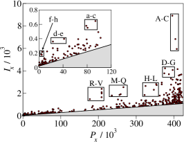
Figure 2: Total influence of papers $I_{x}$ versus their progeny size $P_{x}$ for the APS citation data (for clarity, only $413$ papers with $I_{x}>20+P_{x}/400$ are shown). Details about the marked outliers are given in Tab. 1.

We now illustrate our ideas on the citation data provided by the American Physical Society (APS). This data contains all 449 705 papers published by the APS from 1893 to 2009 together with their citations to the APS journals. To make the data strictly acyclic, we do not consider a small number of citations that are between papers of the same print date; we are then left with 4 672 812 citations. Fig. 2 shows all papers published by the APS after 1940 and reveals an expected linear relationship between $I_{x}$ and $P_{x}$ with several outstanding papers whose influence is much greater than that of other papers of the same progeny size. (Papers published before 1940 are omitted because of the data sparseness which is amplified by the limitation of our data to citations to and from the APS journals.) Table 1 lists the outliers together with scientific prizes as a proxy for their quality. While our results are affected by using only the APS citations, one can conclude that majority of these outlying papers really represents exceptional research. While it is not our goal to rank the papers, one could achieve that for example by dividing $I_{x}$ by the average $I_{x}$ of papers with the same progeny size $P_{x}$, thus making papers of different age comparable.

Id	Title	Authors	Year	Prize	PR	CR
A	Statistics of the Two-Dimensional Ferromagnet…	H. A. Kramers, G.H. Wannier	1941	LM	54	1 645
B	Crystal Statistics in a Two-Dimensional Model…	L. Onsager	1944	NP	8	87
C	Theory of Superconductivity	J. Bardeen, et al.	1957	NP	2	10
D	The Maser–New Type of Microwave Amplifier,…	J. Gordon, et al.	1955	NP	369	14 517
E	Infrared and Optical Masers	A. Schawlow, C. Townes	1958	NP	171	2 108
F	Population Inversion and Continuous Optical Maser	A. Javan et al.	1961	+	169	14 517
G	Dynamical Model of Elementary Particles Based on…	Y. Nambu, G. Jona-Lasinio	1961	NP	24	50
H	Self-Consistent Equations Including Exchange and…	W. Kohn, L. Sham	1965	NP	1	1
I	Inhomogeneous Electron Gas	P. Hohenberg, W. Kohn	1964	MPM	3	2
J	A Model of Leptons	S. Weinberg	1967	NP	6	18
K	Static Phenomena Near Critical Points:…	L. Kadanoff, et al.	1967	MPM	58	355
L	Radiative Corrections as the Origin of Spontaneous…	S. Coleman, E. Weinberg	1973	DM	31	75
M	Scaling Theory of Localization:…	E. Abrahams, et al.	1979	NP	11	24
N	New Measurement of the Proton Gyromagnetic Ratio…	E.R. Williams, P.T. Olsen	1979		150	26 327
O	New Method for High-Accuracy Determination of…	K. Klitzing	1980	NP	32	134
P	Cluster Formation in Two-Dimensional Random Walk	H. Rosenstock, C. Marquardt	1980		109	217 150
Q	Diffusion-Limited Aggregation…	T.A. Witten, L.M. Sander	1981	+	17	64
R	Electronic Structure of BaPb1-XBiXO3	L.F. Mattheiss, D.R. Hamann	1983		106	4 224
S	Bulk Superconductivity at 36 K in La1.8Sr0.2CuO4	R.J. Cava et al.	1987		37	1 086
T	Evidence for Superconductivity above 40 K In…	C.W. Chu et al.	1987		40	606
U	Superconductivity at 93 K in a New Mixed-Phase…	M.K. Wu et al.	1987	+	19	102
V	Self-Organized Criticality: An Explanation of…	P. Bak et al.	1987	+	16	47
a	Teleporting an Unknown Quantum State via…	C.H. Bennett et al.	1993	+	53	26
b	Bose-Einstein Condensation in a Gas of Sodium Atoms	K.B. Davis et al.	1995	NP	63	27
c	Evidence of Bose-Einstein Condensation in…	C.C. Bradley et al.	1995	+	99	51
d	TeV Scale Superstring and Extra Dimensions	G. Shiu, S.-H.H. Tye	1998		216	3 991
e	Small-World Networks: Evidence for a Crossover Picture	M. Barthélémy, L.A.N. Amaral	1999	+	658	9 872
f	Negative Refraction Makes a Perfect Lens	J.B. Pendry	2000	DM	279	192
g	Composite Medium with Simultaneously Negative…	D.R. Smith et al.	2000	+	433	459
h	Statistical Mechanics of Complex Networks	R. Albert, A.-L. Barabási	2002	VNM	112	59

Table 1: An approximately time-ordered list of the papers marked in Fig. 2 (labels agree with those marked in the figure). To evaluate the quality of the list, we indicate the most important prize received by the authors for research pertinent to the listed papers (LM=Lorentz Medal, NP=Nobel Prize, MPM=Max Planck Medal, DM=Dirac Medal, VNM=John Von Neumann Medal). Important prizes are rarely awarded soon after a discovery is made and this bias is well visible in our table. To overcome this, we add an additional distinguishing criterion for prize-free papers: if they are described as pioneering works in a certain domain on Wikipedia, we mark them with $+$. The last two columns show the paper’s ranking given by the Page Rank score when $\alpha=0.5$ (PR) and the citation count (CR). Bold labels correspond to the papers not detectable as outliers in Fig. 3.

Outliers in the $(P_{x},I_{x})$ plane often do not have particularly high citation counts. When we apply the classical PageRank algorithm to our data as in [14], we observe than many of them do not receive high PageRank values. The differences stem, of course, from differences between the algorithms. While PageRank is a reputation metric [20] awarding papers cited by other reputable papers, our approach focuses on the progeny created by each individual paper. In consequence, even a paper which is not directly cited by popular papers can score high if it establishes a new research direction or a school of thought. In this sense, our approach evaluates originality of papers. On the other hand, interdisciplinary works necessarily focus the flow of influence less and hence they are not likely to score high with respect to the $I_{x}/P_{x}$ criterion.

We finally note that the definition of the PageRank score $I^{\alpha}_{x}$ in Eq. 4 allows for a meaningful research of outliers in the $(I^{\alpha}_{x},k^{in}_{x})$ plane (see [14]), similarly as we do in the $(I_{x},P_{x})$ plane for the aggregate impact $I_{x}$. While some papers appear as outliers in both planes, there are some significant differences which further demonstrate the distinction between our evaluation metric and the PageRank (see Fig. 3). These differences, marked with bold letters in Table 1, correspond to relatively recent but seminal papers, suggesting that our method is more effective in removing the inherent time bias of citation data discussed above.

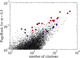
Figure 3: PageRank with $\alpha=0.5$ vs citation count (with an older version of the APS data, a similar plot was already presented in [14]). Outliers from Fig. 2 are marked either with red squares (if they can be considered as outliers also in this figure) and with blue crosses (if they are not outliers here—these papers have their number written in bold in Table 1).

After showing that our concept of influence quantified by the $\mathsf{G}$ matrix has its merit, we use it to evaluate similarity of papers. The basic idea is that papers $x$ and $y$ are similar if they are influenced by the same works (they have similar “genetic” composition). To evaluate this similarity we take

$$S^{*}(x,y)=\sum_{i}\sqrt{G_{ix}G_{iy}}.$$ (5)

It is also possible to base the similarity on $\min\{G_{ix},G_{iy}\}$ or $G_{ix}G_{iy}$, for example—we present here the choice performing best in our numerical tests. Note that this similarity is not normalized: its lower bound is zero but the upper bound is bounded only by $\mathcal{A}_{x}\cap\mathcal{A}_{y}$. We stress that $S^{*}$ is parameter-free and hence practical to use.

The standard way to evaluate a similarity metric is to test how well it is able to reproduce missing links in a network [21, 22]. In practice this means that small part of links (usually $10\%$) is removed from the network and one attempts to guess the removed links by seeing which similar nodes are not connected. A similarity metric which is able to “repair” well the network presumably captures well the network’s structure and one may use it also for other purposes than link prediction. In the case of our similarity metric $S^{*}$, we adopt a slightly different approach: we test how good recommendations it is able to provide to selected individuals. This change is motivated by potential practical use of such recommendations for scientists who often face the problem of searching for relevant literature in their research field [24].

Our tests are done as follows. We first divide the data in two parts: papers published until year 2003 (the sample set—it contains approximately $75\%$ of all papers) and those published after 2003 (the probe set). Then we find 20 most-cited articles published in each core APS journal in 2003 (we consider seven journals: Phys. Rev. Lett., Rev. Mod. Phys. and Phys. Rev. A–E) and take their last authors if they published at least one paper with the APS after 2003. Recommendations are made for each test author separately on the basis of papers published by this author in 2003. Denoting the set of papers published by author $\alpha$ in 2003 as $\mathcal{U}_{\alpha}$, the recommendation score of paper $x$ is given by its similarity with all $y$ in this set

$$r_{x}=\sum_{y\in\mathcal{U}_{\alpha}}S^{*}(x,y).$$ (6)

Papers that haven’t been cited by author $\alpha$ until 2003 are then sorted according to their score in a descending order and those at the top represent personalized recommendation for this author.

Resulting recommendations are evaluated using the probe set which allows us to label as “relevant” those papers that were eventually cited by a given author after 2003. To curb the level of noise in the results, we discard authors with less than $10$ relevant papers to be guessed. Then we are left with the final set of $99$ test authors who have on average $116$ relevant items to be guessed out of almost $340\,000$ papers published until 2003. To assess the recommendations, we use metrics often used in the field of recommender systems [16]: (i) precision $P_{100}$ (the fraction of the top 100 places of the recommendation list occupied by the relevant papers), (ii) recall $R_{100}$ (the fraction of the relevant papers appearing at the top 100 places of the recommendation list), (iii) the average ranking of the relevant papers $q_{R}$ (expressed as a fraction of all potentially relevant papers), and (iv) the fraction of the relevant papers with non-zero score $f_{R}$. A good recommendation list should have relevant papers at the top, i.e., high $P_{100}$ and $R_{100}$ and low $q_{R}$, and it should assign non-zero scores to most relevant papers, e.g. high $f_{R}$ (all these quantities lie in the range $[0,1]$).

To test our similarity, we compare its performance in a recommendation process with other similarity metrics. Based on results presented in [22], we have selected three highly performing metrics: the Common Neighbors similarity (CN), the Resource Allocation Index (RA), and the Katz-based similarity (KA). Since they are all defined on undirected networks, we evaluate them assuming that all links in our data are undirected. CN simply counts the number of common neighbors for a pair of nodes. RA does the same but it values less common neighbors with many connections,

$$S^{RA}(x,y)=\sum_{z\in\Gamma(x)\cap\Gamma(y)}\lvert\Gamma(z)\rvert^{-1}$$ (7)

where $\Gamma(x)$ is the set of direct neighbors of node $x$. We finally employ a commonly used similarity, KA, which counts the number of paths between two given nodes with individual paths weighted exponentially less according to their length (this similarity has a close relation with the Katz centrality measure [23]). Denoting the network’s adjacency matrix with $\mathsf{A}$, KA can be written in the form of a series

$$S^{KA}(x,y)=\sum_{i=1}^{\infty}\beta^{i}(\textsf{A}^{i})_{xy}.$$ (8)

In our case, we use $\beta=0.75$ which yields slightly superior performance. Local similarities $S^{CN}$ and $S^{RA}$ are computationally considerably less demanding than global (based on the whole network) similarities $S^{*}$ and $S^{KA}$. For practical reasons, we limit the computation of $S^{*}$ to papers that are not more than six steps from both $x$ and $y$. For $S^{KA}$, we limit its summation to the order $\mathsf{A}^{12}$ (see Fig. 4 for how these restrictions affect the results).

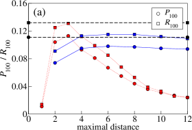
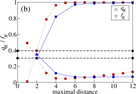
Figure 4: Precision and recall (a) and average ranking of relevant items and fraction of ranked relevant items (b) for $S^{KA}$ (red symbols, dotted lines), $S^{*}$ (blue symbols, solid lines) and $S^{RA}$ (black symbols, dashed lines). $S^{KA}$ shows a strong dependency on the maximal distance with best $P_{100}$ and $R_{100}$ achieved when the maximal distance is $3$. However, $q_{R}$ is only $0.79$ at this point which means that at this level of truncation, it represents a transition between local and global similarity metrics. When all powers of $\mathsf{A}$ are included, $S^{KA}$ performs poorly with respect to all measured characteristics but $f_{R}$. By contrast, the performance of $S^{*}$ decreases only slightly when the maximal distance is above eight.

Similarities described above can be substituted for $S^{*}(x,y)$ in Eq. (6), leading to recommendations which can be in turn compared with those obtained with $S^{*}$. Test results can be found in Fig. 4 where we plot performances of different algorithms vs the maximal distance used to compute global similarities. Results for the Resource Allocation Index are indicated with flat lines while results for the Common Neighbor similarity are omitted because they are always worse than for $RA$. In general we see a good performance of $S^{RA}$ with respect to precision and recall. This is because local metrics rank only a small set of papers (local neighborhoods) where there is high probability of finding relevant papers. The drawback is that only a minor part of relevant papers is found ($f_{R}\approx 0.4$) and their average ranking is poor ($q_{R}\approx 0.3$).

At the same time, global metrics $S^{*}$ and $S^{KA}$ are able to rank almost all relevant objects and achieve much lower average ranking, but they pay for this enhanced ’variety’ with worse performance at top places of their recommendation lists. When the maximal distance of five or more is considered (which is necessary for making $S^{KA}$ a truly global similarity metric with $f_{R}\approx 1$, $S^{*}$ significantly outperforms $S^{KA}$ and, from the point of view of recommendation, provides a good compromise between global and local metrics. This is despite the fact that $S^{KA}$ and $S^{RA}$ are computed on undirected data which gives them access to more information: they assign similarity also to nodes with overlapping progeny, not only to those with overlapping ancestors as $S^{*}$ does. Further tests show that if we prevent $S^{RA}(x,y)$ from accessing this information, its precision and recall decrease to $0.104$ and $0.124$ respectively which is comparable to the results obtained with $S^{*}$. We may conclude that $S^{*}$ is a reliable similarity metric which is able to compete with other known metrics.

In conclusion, our results unveil the value of the passage probability in random walks on DAGs. On the example of scientific citations we showed that it allows us to quantify the influence of a given paper (node) on the others, to identify seminal and innovative papers (i.e., instrumental nodes of the network), and to introduce a similarity metric whose performance is comparable with that of other state-of-the-art metrics. In this Letter, we aimed at simplicity and hence we didn’t consider additional effects that may have impact on the interpretation of the analyzed citation data. For example, we didn’t consider that every paper relies on general knowledge which is however never cited. To reflect that, one could for example add an artificial node referred by every other node in the network and repeat the same analysis as we did. Further, similarly as for PageRank [25], our framework also lends itself to generalizations based on assigning past citations with lower weights to better reflect current relevance or, more generally, trends. We believe that our framework might prove useful well beyond citation networks as it opens possibilities for the investigation of asymmetric interactions in DAGs by exploiting their intrinsic acyclic nature. The presented ideas and tools can be readily applied to citation networks related to any kind of intellectual production such as patents and legal cases. Similar networks of dependency relations can also be found in biology (phylogenetic networks and food webs, for example) as well as in other systems that can be mapped into a DAG, where individuation of fundamental nodes and estimation of dependency relations within the graph can be useful and non-trivial tasks.

- [1] \NameM. E. J. Newman \REVIEWSIAM Review452003167.
- [2] \NameD. J. Watts \REVIEWAnnual Review of Sociology302004243.
- [3] \NameM. C. González A.-L. Barabási \REVIEWNature Physics32007224.
- [4] \NameS. H. Strogatz \REVIEWNature4102001268.
- [5] \NameS. N. Dorogovtsev, A. V. Goltsev, J. F. F. Mendes \REVIEWRev. of Mod. Phys.8020081275.
- [6] \NameM. O. Jackson \BookSocial and Economic Networks \PublPrinceton Univ. Press \Year2008.
- [7] \NameA. N. Langville C. D. Meyer \BookGoogle’s PageRank and Beyond: The Science of Search Engine Rankings \PublPrinceton Univ. Press \Year2006.
- [8] \NameT. Zhou et al. \REVIEWPNAS10720104511.
- [9] \NameM. Altmann \REVIEWSoc. Networks1519931.
- [10] \NameF. Fouss et al. \REVIEWIEEE Trans. Knowl. Data Eng.192007355.
- [11] \NameW. R. Young, A. J. Roberts G. Stuhne \REVIEWNature4122001328.
- [12] \NameB. Karrer M. E. J. Newman \REVIEWPhys. Rev. Lett.1022009128701.
- [13] \NameB. Karrer M. E. J. Newman \REVIEWPhys. Rev. E802009046110.
- [14] \NameP. Chen et al. \REVIEWJournal of Informetrics120078.
- [15] \NameM. Franceschet \REVIEWComm. of the ACM54201192.
- [16] \NameG. Adomavicius A. Tuzhilin \REVIEWIEEE Trans. Knowl. Data Eng.172005734.
- [17] \NameA. Jaffe M. Trajtenberg \BookPatents, Citations and Innovations: A Window on the Knowledge Economy \PublMIT Press \Year2002.
- [18] \NameJ. H. Fowler et al. \REVIEWPolitical Analysis152007324.
- [19] \NameN. Gilbert \REVIEWSoc. Res. Online219972.
- [20] \NameA. Jøsang, R. Ismail C. Boyd \REVIEWDecision Supp. Syst.432007618.
- [21] \NameD. Liben-Nowell J. Kleinberg \REVIEWJ. of the Am. Soc. Inf. Sci. and Tech.5820101019.
- [22] \NameL. Lü T. Zhou \REVIEWPhysica A39020111150.
- [23] \NameL. Katz \REVIEWPsychometrika18195339.
- [24] \NameS. M. McNee et al. \BookProceedings of ACM CSCW \PublACM \Year2002 \Page116.
- [25] \NameD. Walker et al. \ReviewJ. Stat. Mech. \Year2007 \PageP06010.