Spooky action at a distance in general probabilistic theories

Abstract

We call a probabilistic theory “complete” if it cannot be further refined by no-signaling hidden-variable models, and name a theory “spooky” if every equivalent hidden-variable model violates Shimony’s Outcome Independence. We prove that a complete theory is spooky if and only if it admits a pure steering state in the sense of Schrödinger. Finally we show that steering of complementary states leads to a Schrödinger’s cat-like paradox.

1 Introduction

Since the early days physicists have been wondering whether Quantum Theory (QT) can be considered complete [1, 2], or more refined theories compatible with quantum predictions could exist. These models, also known as Hidden Variable Theories (HVT), reproduce QT thanks to a statistical definition of pure quantum states, which are obtained as averages over the more fundamental states of the HVT. In this approach, which reduces QT to a Statistical Mechanics, many results have been obtained, such as the theorems by Kochen-Specker and Bell [3, 4], and the results by Conway-Kochen on the free will [5, 6].

Recently, General Probabilistic Theories (GPT) have received great attention as the appropriate framework to study foundational aspects of physics [7, 8, 9, 10, 11, 12, 13]. Despite much work has been devoted to the relations between probabilistic theories and HVTs, these results are mostly a characterization of the probability measures, lacking a conceptual physical characterization of the theory itself, for example in terms of axioms. So far there exist examples of probability measures that do not respect locality, signaling, non-contextuality, determinism, completeness, etc., but none of these highlights the physical properties that a GPT must fulfill in order to achieve such violations.

The present Letter breaks the ground in the direction of providing a characterization theorem for complete “spooky” theories (see definitions in the following). Roughly speaking, the spookiness of a complete theory is the apparent “action at a distance” due to outcome correlations [14]. We show that spookiness for complete theories is equivalent to Schrödinger’s steering property [15, 16]. We do not discuss the completeness assumption since an exhaustive inquiry would require a much more complicate analysis, comparable to a generalized Bell theorem for GPTs. Finally, we use the results about spookiness to prove that complementarity and steering are necessary and sufficient conditions to raise a Schrödinger’s cat-like paradox.

2 Hidden variable theories for a GPT

The most important feature of a given probabilistic theory—such as QT or more generally any GPT—is the probability rule that links the various elements of the theory itself. More precisely, given a state $\rho$, a group of observers for the theory ($A,B,C,\dots$) and the measurements $a,b,c,\dots$ that $A,B,C,\dots$ perform, the probability rule $\operatorname{Pr}\!\left[a_{i},b_{j},c_{k},\dots\vphantom{a,b,c,\dots\rho}\right|\left.a,b,c,\dots\rho\vphantom{a_{i},b_{j},c_{k},\dots}\right]$ is defined for every possible outcome $a_{i},b_{j},c_{k},\dots$ over a suitable sample space $\Omega$. In the remainder of the Letter, we will drop the explicit dependence of all probablity rules on the state $\rho$. We can now define a hidden variable description for the previous model as follows.

Definition 1 (Hidden Variable Theory).

An equivalent HVT for a GPT is given by a set $\Lambda\ni\lambda$, and a probability rule $\widetilde{\operatorname{Pr}}\!\left[\cdot\vphantom{\cdot}\right|\left.\cdot\vphantom{\cdot}\right]$ on $\Omega\times\Lambda$, such that [17]

$$\operatorname{Pr}\!\left[a_{i},b_{j},c_{k},\dots\vphantom{a,b,c,\dots}\right|\left.a,b,c,\dots\vphantom{a_{i},b_{j},c_{k},\dots}\right]=$$ (1)

$$\sum_{\lambda}\widetilde{\operatorname{Pr}}\!\left[a_{i},b_{j},c_{k},\dots\vphantom{a,b,c,\dots,\lambda}\right|\left.a,b,c,\dots,\lambda\vphantom{a_{i},b_{j},c_{k},\dots}\right]\widetilde{\operatorname{Pr}}\!\left[\lambda\vphantom{a,b,c,\dots}\right|\left.a,b,c,\dots\vphantom{\lambda}\right].$$

for every state of the GPT.

In the following we will restrict our attention to HVTs satisfying two requirements: $\lambda$-independence, namely $\widetilde{\operatorname{Pr}}\!\left[\lambda\vphantom{a,b,c,\dots}\right|\left.a,b,c,\dots\vphantom{\lambda}\right]=\widetilde{\mathrm{Pr}}[\lambda]$, i.e. $\lambda$ is an objective parameter independent of the choice of measurements ; and parameter independence, namely $\widetilde{\operatorname{Pr}}\!\left[a_{i}\vphantom{a,b,c,\dots,\lambda}\right|\left.a,b,c,\dots,\lambda\vphantom{a_{i}}\right]=\widetilde{\operatorname{Pr}}\!\left[a_{i}\vphantom{a,\lambda}\right|\left.a,\lambda\vphantom{a_{i}}\right]$ and similarly for $b$, $c$, $\dots$, i.e. the HVT is no-signaling. Clearly, given a GPT, without these two restrictions we can always build an equivalent deterministic HVT which is signaling, and denies observers’ free choice [17].

A GPT is complete if every equivalent HVT provides no further descriptive detail. Besides classical probability theory, there is at least a GPT that is complete in the present sense, which is indeed Quantum Theory, as proved recently by Colbeck and Renner in Ref. [19].

It is now crucial to require that probabilities depend non-trivially on the hidden variable.

Definition 2 (Descriptively significant HVT).

A HVT is descriptively significant for an equivalent GPT if it satisfies $\lambda$-independence and parameter independence, and there exists a pure state and measurements $a,b,\dots,a_{i},b_{j},\dots$ such that for some $\lambda,\lambda^{\prime}\in\Lambda$ with $\widetilde{\operatorname{Pr}}\!\left[a_{i},b_{j},\dots\vphantom{a,b,\dots,\lambda}\right|\left.a,b,\dots,\lambda\vphantom{a_{i},b_{j},\dots}\right]\neq 0$, one has

$$\widetilde{\operatorname{Pr}}\!\left[a_{i},b_{j},\dots\vphantom{a,b,\dots,\lambda}\right|\left.a,b,\dots,\lambda\vphantom{a_{i},b_{j},\dots}\right]\neq\widetilde{\operatorname{Pr}}\!\left[a_{i},b_{j},\dots\vphantom{a,b,\dots,\lambda^{\prime}}\right|\left.a,b,\dots,\lambda^{\prime}\vphantom{a_{i},b_{j},\dots}\right].\!\!\!$$ (2)

Definition 3 (Complete GPT).

A GPT is complete if every equivalent HVT is not descriptively significant.

The reason why it is important to investigate only descriptively significant HVTs is the following. Given a non significant HVT for a given GPT, for all pure states and all $a,b,\dots,a_{i},b_{j},\dots$, we have that, by Eq.(2) and Eq.(1)

$$\operatorname{Pr}\!\left[a_{i},b_{j},\dots\vphantom{a,b,\dots}\right|\left.a,b,\dots\vphantom{a_{i},b_{j},\dots}\right]=\widetilde{\operatorname{Pr}}\!\left[a_{i},b_{j},\dots\vphantom{a,b,\dots,\lambda_{i}}\right|\left.a,b,\dots,\lambda_{i}\vphantom{a_{i},b_{j},\dots}\right],$$ (3)

for all $\lambda_{i}\in\Lambda$ such that $\widetilde{\operatorname{Pr}}\!\left[a_{i},b_{j},\dots\vphantom{a,b,\dots,\lambda_{i}}\right|\left.a,b,\dots,\lambda_{i}\vphantom{a_{i},b_{j},\dots}\right]\neq 0$. Therefore, we conclude that $\widetilde{\operatorname{Pr}}\!\left[a_{i},b_{j},\dots\vphantom{a,b,\dots,\lambda_{i}}\right|\left.a,b,\dots,\lambda_{i}\vphantom{a_{i},b_{j},\dots}\right]$ shares all the features of $\operatorname{Pr}\!\left[a_{i},b_{j},\dots\vphantom{a,b,\dots}\right|\left.a,b,\dots\vphantom{a_{i},b_{j},\dots}\right]$, e.g. non locality or complementarity.

Given a GPT, among all HVTs equivalent to it and not descriptively significant, there is one theory that enjoys the so-called “single-valuedness property” [17].

Definition 4 (Single-valuedness).

A HVT satisfies the single-valuedness property if $\left|\Lambda\right|=1$.

For a HVT with single-valuedness there exists only one hidden variable value $\lambda_{0}$, whence for every $i$ and $j$, $\operatorname{Pr}\!\left[a_{i},b_{j}\vphantom{a,b}\right|\left.a,b\vphantom{a_{i},b_{j}}\right]\equiv\widetilde{\operatorname{Pr}}\!\left[a_{i},b_{j}\vphantom{a,b,\lambda_{0}}\right|\left.a,b,\lambda_{0}\vphantom{a_{i},b_{j}}\right]$. Given a GPT there is always an equivalent hidden variable model which satisfies single-valuedness [17]: this fact recalls the intuition that QT can be regarded itself as a HVT, where the hidden variable role is played by the quantum state. If we want to study a complete probabilistic theory it is useful to refer to the simplest non descriptively significant equivalent hidden variable model, that is the one which satisfies single-valuedness.

Thanks to J. P. Jarrett [20], it is known that the Bell locality [3] is equivalent to the conjunction of two different properties: the aforementioned Parameter Independence and the Shimony’s so-called Outcome Independence [21]. Parameter independence corresponds to the property of “no-signaling without exchange of physical systems” in [9] for GPTs, while Outcome Independence can be stated as the factorizability of joint probabilities, i.e. 

$$\widetilde{\operatorname{Pr}}\!\left[a_{i},b_{j}\vphantom{a,b,\lambda}\right|\left.a,b,\lambda\vphantom{a_{i},b_{j}}\right]=\widetilde{\operatorname{Pr}}\!\left[a_{i}\vphantom{a,b,\lambda}\right|\left.a,b,\lambda\vphantom{a_{i}}\right]\times\widetilde{\operatorname{Pr}}\!\left[b_{j}\vphantom{a,b,\lambda}\right|\left.a,b,\lambda\vphantom{b_{j}}\right].$$ (4)

Notice that the previous definition can be applied to a general GPT, regarded as a single-valued HVT.

The EPR paradox can be rewritten in the following similar way [22, 17]: quantum predictions are not compatible with any equivalent non descriptively significant HVT which satisfies Outcome Independence. For this reason, according to EPR, QT presents a spooky action at a distance. We now want to extend the EPR result, namely: which are the GPTs that present this spooky flavor? First we must define in what sense a theory can present spooky features.

Definition 5 (Spooky theory).

A GPT is spooky if it violates outcome independence on a pure state and every equivalent descriptively significant HVT does so.

From now on, we will focus on complete spooky GPTs, unless told otherwise.

3 Review of general probabilistic theories

Before starting we need to introduce the usual notation for GPTs. For a detailed discussion see [7]. The symbols $\rho_{A}$, $\left|\rho\right)_{A}$ and denote the state $\rho$ for system $A$, representing the information about the system initialization, including the probability that such preparation can occur. The set of the states of a given system $A$ is a (truncated) positive cone, and therefore given the states $\{\rho_{i}\}_{i\in\eta}$ for $A$, every their convex combination belongs to the cone of the states of $A$. The extremal rays of the cone—namely the states which cannot be seen as a convex combination of other ones—are the so called pure states.

Similarly, $c_{iA}$, $\left(c_{i}\right|_{A}$ and mean the effect $c_{i}$ for system $A$ or, in more practical terms, the $i$-th outcome of the test (measurement) $c=\{c_{i}\}_{i\in\eta}$ on system $A$. Given a system $A$, its effects are bounded linear positive functionals from the states of $A$ to $\left[0,1\right]\subset\mathbb{R}$, and therefore they belong to the dual cone of the cone of the states. The application of the effect $c_{i}$ on the state $\rho$ is written as $(c_{i}|\rho)_{A}$ or , and it means the probability that the outcome of measure $c$ performed on the state $\rho$ of system $A$ is $c_{i}$, i.e. $(c_{i}|\rho)_{A}:=\operatorname{Pr}\!\left[c_{i}\vphantom{c}\right|\left.c\vphantom{c_{i}}\right]$. In the following we will not specify the system when it is clear from the context or it is generic.

The symbol $e_{A}$ will denote a deterministic effect for system $A$, namely a measurement with a single outcome. For any state $\sigma$, the symbol $(e|\sigma)$ denotes its preparation probability within a test including a measurement $\{c_{i}\}_{i\in\eta}$ such that $e=\sum_{i\in\eta}c_{i}$. A state $\sigma$ is deterministic if we know with certainty that it has been prepared in any test, whence $(e|\sigma)=1$ for every deterministic effect $e$. An ensemble is a collection of (possibly non-deterministic) states $\{\alpha_{i}\}_{i\in\eta}$ such that $\rho:=\sum_{i\in\eta}\alpha_{i}$ is deterministic. A GPT is causal (i.e. it satisfies the no-signaling from the future axiom [7]) iff the deterministic effect is unique. Thanks to this last feature, in a causal GPT the preparation probability for the state $\sigma$ is well defined since it is independent of the tests following the preparation. For this reason, for every state $\rho$ we can always consider the deterministic state $\bar{\rho}:=(e|\rho)\rho$, or, in other words, in a causal theory evey state is proportional to a deterministic one. In the following, we will consider a general causal GPT.

4 Spookiness, steering and completeness

In this section we will show our main results. Let $\rho$ be a joint deterministic state for systems $A$ and $B$. Let $a_{0}$, $a_{1}$ be two effects for $A$ forming a so-called complete test: namely, for every state $\sigma$ of $A$ we have $(a_{0}|\sigma)+(a_{1}|\sigma)=(e|\sigma)$. Similarly, let the effects $b_{0}$, $b_{1}$ form a complete test for $B$. Let us define the following useful shorthand

$$p_{ij}:=\operatorname{Pr}\!\left[a_{i},b_{j}\vphantom{a,b}\right|\left.a,b\vphantom{a_{i},b_{j}}\right]\equiv\begin{aligned} \lx@xy@svg{\hbox{\raise 0.0pt\hbox{\kern 7.58508pt\hbox{\ignorespaces\ignorespaces\ignorespaces\hbox{\vtop{\kern 0.0pt\offinterlineskip\halign{\entry@#!@&&\entry@@#!@\cr&&\\&&\crcr}}}\ignorespaces{\hbox{\kern-7.58508pt\raise 0.0pt\hbox{\hbox{\kern 5.00002pt\raise-1.18056pt\hbox{$\textstyle{\hphantom{\rho}}$}}}}}\ignorespaces\ignorespaces\ignorespaces\ignorespaces{\hbox{\kern-2.58507pt\raise-6.85226pt\hbox{\hbox{\kern 0.0pt\raise-1.18056pt\hbox{$\textstyle{\rho}$}}}}}\ignorespaces\ignorespaces\ignorespaces\ignorespaces\ignorespaces\ignorespaces{\hbox{\lx@xy@droprule}}\ignorespaces\ignorespaces\ignorespaces\ignorespaces\ignorespaces{\hbox{\lx@xy@droprule}}\ignorespaces\ignorespaces\ignorespaces\ignorespaces\ignorespaces\ignorespaces{\hbox{\lx@xy@droprule}}\ignorespaces\ignorespaces\ignorespaces\ignorespaces\ignorespaces\ignorespaces\ignorespaces{\hbox{\lx@xy@droprule}}\ignorespaces{\hbox{\kern-7.58508pt\raise 7.62495pt\hbox{\hbox{\kern 0.0pt\raise-8.99994pt\hbox{$\textstyle{\hbox{\cirbuild@}}$}}}}}\ignorespaces{\hbox{\kern-7.58508pt\raise-21.32948pt\hbox{\hbox{\kern 0.0pt\raise 8.99994pt\hbox{$\textstyle{\hbox{\cirbuild@}}$}}}}}{\hbox{\kern 5.0pt\raise 0.0pt\hbox{\hbox{\kern-2.625pt\raise 1.00006pt\hbox{$\textstyle{\scriptstyle A}$}}}}}\ignorespaces\ignorespaces\ignorespaces\ignorespaces{}{\hbox{\lx@xy@droprule}}\ignorespaces{}{\hbox{\lx@xy@droprule}}{\hbox{\kern 9.28125pt\raise 0.0pt\hbox{\hbox{\kern 0.0pt\raise 0.0pt\hbox{$\textstyle{\lx@xy@svgnested{\hbox{\raise 0.0pt\hbox{\kern 12.21516pt\hbox{{\hbox{\kern-6.10757pt\raise 0.0pt\hbox{\hbox{\kern 2.5pt\raise-1.22945pt\hbox{$\textstyle{\vphantom{\rule{0.0pt}{1.00006pt}a_{i}}}$}}}}}{\hbox{\kern-6.10759pt\raise 0.0pt\hbox{\hbox{\kern 0.0pt\raise 0.0pt\hbox{\cirbuild@}}}}}\ignorespaces{\hbox{\kern-7.21516pt\raise 0.0pt\hbox{\hbox{\kern 0.0pt\raise-1.22945pt\hbox{$\textstyle{a_{i}}$}}}}}\ignorespaces\ignorespaces\ignorespaces\ignorespaces\ignorespaces{\hbox{\kern-12.21516pt\raise 6.10759pt\hbox{\hbox{\kern 0.0pt\raise-1.22945pt\hbox{$\textstyle{\hphantom{a_{i}}}$}}}}}\ignorespaces\ignorespaces\ignorespaces{\hbox{\lx@xy@droprule}}\ignorespaces\ignorespaces\ignorespaces\ignorespaces\ignorespaces{\hbox{\kern-12.21516pt\raise-6.10759pt\hbox{\hbox{\kern 0.0pt\raise-1.22945pt\hbox{$\textstyle{\hphantom{a_{i}}}$}}}}}\ignorespaces\ignorespaces\ignorespaces{\hbox{\lx@xy@droprule}}\ignorespaces\ignorespaces\ignorespaces{\hbox{\kern-12.21516pt\raise 6.10759pt\hbox{\hbox{\kern 0.0pt\raise-1.22945pt\hbox{$\textstyle{\hphantom{a_{i}}}$}}}}}\ignorespaces\ignorespaces\ignorespaces{\hbox{\kern-12.21516pt\raise-6.10759pt\hbox{\hbox{\kern 0.0pt\raise-1.22945pt\hbox{$\textstyle{\hphantom{a_{i}}}$}}}}}\ignorespaces\ignorespaces\ignorespaces{\hbox{\lx@xy@droprule}}}}}}}$}}}}}\ignorespaces\ignorespaces\ignorespaces\ignorespaces{}{\hbox{\lx@xy@droprule}}\ignorespaces{}{\hbox{\lx@xy@droprule}}{\hbox{\lx@xy@droprule}}{\hbox{\kern-7.58508pt\raise-13.70451pt\hbox{\hbox{\kern 5.00002pt\raise-1.18056pt\hbox{$\textstyle{\hphantom{\rho}}$}}}}}{\hbox{\kern 5.0pt\raise-13.70451pt\hbox{\hbox{\kern-2.83037pt\raise 1.00006pt\hbox{$\textstyle{\scriptstyle B}$}}}}}\ignorespaces\ignorespaces\ignorespaces\ignorespaces{}{\hbox{\lx@xy@droprule}}\ignorespaces{}{\hbox{\lx@xy@droprule}}{\hbox{\kern 8.76346pt\raise-13.70451pt\hbox{\hbox{\kern 0.0pt\raise 0.0pt\hbox{$\textstyle{\lx@xy@svgnested{\hbox{\raise 0.0pt\hbox{\kern 11.91833pt\hbox{{\hbox{\kern-7.43999pt\raise 0.0pt\hbox{\hbox{\kern 3.98082pt\raise-2.00446pt\hbox{$\textstyle{\vphantom{\rule{0.0pt}{1.00006pt}b_{j}}}$}}}}}{\hbox{\kern-7.44pt\raise 0.0pt\hbox{\hbox{\kern 0.0pt\raise 0.0pt\hbox{\cirbuild@}}}}}\ignorespaces{\hbox{\kern-6.91833pt\raise 0.0pt\hbox{\hbox{\kern 0.0pt\raise-2.00446pt\hbox{$\textstyle{b_{j}}$}}}}}\ignorespaces\ignorespaces\ignorespaces\ignorespaces\ignorespaces{\hbox{\kern-11.91833pt\raise 7.44pt\hbox{\hbox{\kern 0.0pt\raise-2.00446pt\hbox{$\textstyle{\hphantom{b_{j}}}$}}}}}\ignorespaces\ignorespaces\ignorespaces{\hbox{\lx@xy@droprule}}\ignorespaces\ignorespaces\ignorespaces\ignorespaces\ignorespaces{\hbox{\kern-11.91833pt\raise-7.44pt\hbox{\hbox{\kern 0.0pt\raise-2.00446pt\hbox{$\textstyle{\hphantom{b_{j}}}$}}}}}\ignorespaces\ignorespaces\ignorespaces{\hbox{\lx@xy@droprule}}\ignorespaces\ignorespaces\ignorespaces{\hbox{\kern-11.91833pt\raise 7.44pt\hbox{\hbox{\kern 0.0pt\raise-2.00446pt\hbox{$\textstyle{\hphantom{b_{j}}}$}}}}}\ignorespaces\ignorespaces\ignorespaces{\hbox{\kern-11.91833pt\raise-7.44pt\hbox{\hbox{\kern 0.0pt\raise-2.00446pt\hbox{$\textstyle{\hphantom{b_{j}}}$}}}}}\ignorespaces\ignorespaces\ignorespaces{\hbox{\lx@xy@droprule}}}}}}}$}}}}}\ignorespaces\ignorespaces\ignorespaces\ignorespaces{}{\hbox{\lx@xy@droprule}}\ignorespaces{}{\hbox{\lx@xy@droprule}}{\hbox{\lx@xy@droprule}}\ignorespaces}}}}\ignorespaces\end{aligned}. \textstyle{\rho} \textstyle{\scriptstyle A} \textstyle{a_{i}} \textstyle{\scriptstyle B} \textstyle{b_{j}} \textstyle{\rho} \textstyle{\scriptstyle A} \textstyle{a_{i}} \textstyle{\scriptstyle B} \textstyle{b_{j}}$$ (5)

The number $p_{ij}$ represents the probability that Alice and Bob obtain respectively the $i$-th and the $j$-th outcome while performing measurements $a$ and $b$ on the state $\rho$.

Under these assumptions the following theorems hold.

Theorem 1.

A complete GPT is spooky if and only if there exists a pure state $\rho$ of $AB$ and tests $\{a_{0},a_{1}\}$ of $A$ and $\{b_{0},b_{1}\}$ of $B$ such that the probabilities $p_{ij}$ of Eq. (5) satisfy the following constraint:

$$p_{00}\ p_{11}\neq p_{01}p_{10}.$$ (6)

Proof.

A complete GPT is spooky iff it has a test $\left\{a_{0},a_{1}\right\}$ for system $A$, a test $\{b_{0},b_{1}\}$ for system $B$, and pure state $\rho$ for $AB$ such that $p_{ij}$ is not factorized. This is equivalent to the requirement that the matrix $p_{ij}$ has rank larger than one, namely for a $2\times 2$ matrix the determinant of the matrix is non vanishing, i.e. Eq. (6) holds. $\,\blacksquare$

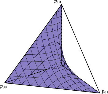
Figure 1: The tetrahedron (outlined in thick black line) represents the set of possible values of probabilities $p_{00}$, $p_{01}$, $p_{10}$ satisfying the normalization condition. The hyperbolic paraboloid identifies the probabilities that satisfy Outcome Independence.

The theorem states that if we describe by a pure state of a GPT an experiment with probabilities given by Eq.(6), then we can not provide a local explanation for the observed physical phenomenon.

Notice that the previous result does not manifestly require any choice by the observers, since it needs only one test for each subsystem. Consequently, there are no explicit assumptions about the observers’ free will, thus extending Brandenburger–Yanofsky’s reformulation of the EPR paradox [17]. One may wonder how such non-locality can be proved without observers’ choice between “complementary” measurements. The answer resides in the completeness requirement. Clearly a GPT with only one measurement for each observer always admits an equivalent HVT, which is the deterministic one, since there is no requirement for parameter independence and $\lambda$-independence.

Generally, requiring $0\leq p_{ij}\leq 1$ and $\sum p_{ij}=1$ implies that $p_{00}$, $p_{01}$, $p_{10}$ must lie in the tetrahedron outlined in figure 1 ($p_{11}$ is simply obtained by the normalization condition). The spookiness condition, namely Eq. (6), defines a hyperbolic paraboloid, and all spooky theories give rise to points of the tetrahedron that do not lie on the surface of the paraboloid.

We now prove a theorem that along with Theorem 1 provides the main result in this Letter. The following theorem pertains to the property of steering [15, 16] for a GPT, that we briefly recall here.

Definition 6 (Steering state for an ensemble).

The state $\rho$ of the system $AB$ steers the ensemble $\{p_{i}\alpha_{i}\}_{i\in\eta}$ of states of the system $A$ if there exists a test $\{b_{i}\}_{i\in\eta}$ of the system $B$ such that

$$\begin{aligned} \lx@xy@svg{\hbox{\raise 0.0pt\hbox{\kern 7.58508pt\hbox{\ignorespaces\ignorespaces\ignorespaces\hbox{\vtop{\kern 0.0pt\offinterlineskip\halign{\entry@#!@&&\entry@@#!@\cr&&\\&&\crcr}}}\ignorespaces{\hbox{\kern-7.58508pt\raise 0.0pt\hbox{\hbox{\kern 5.00002pt\raise-1.18056pt\hbox{$\textstyle{\hphantom{\rho}}$}}}}}\ignorespaces\ignorespaces\ignorespaces\ignorespaces{\hbox{\kern-2.58507pt\raise-11.95804pt\hbox{\hbox{\kern 0.0pt\raise-1.18056pt\hbox{$\textstyle{\rho}$}}}}}\ignorespaces\ignorespaces\ignorespaces\ignorespaces\ignorespaces\ignorespaces{\hbox{\lx@xy@droprule}}\ignorespaces\ignorespaces\ignorespaces\ignorespaces\ignorespaces{\hbox{\lx@xy@droprule}}\ignorespaces\ignorespaces\ignorespaces\ignorespaces\ignorespaces\ignorespaces{\hbox{\lx@xy@droprule}}\ignorespaces\ignorespaces\ignorespaces\ignorespaces\ignorespaces\ignorespaces\ignorespaces{\hbox{\lx@xy@droprule}}\ignorespaces{\hbox{\kern-7.58508pt\raise 7.62495pt\hbox{\hbox{\kern 0.0pt\raise-8.99994pt\hbox{$\textstyle{\hbox{\cirbuild@}}$}}}}}\ignorespaces{\hbox{\kern-7.58508pt\raise-31.54103pt\hbox{\hbox{\kern 0.0pt\raise 8.99994pt\hbox{$\textstyle{\hbox{\cirbuild@}}$}}}}}{\hbox{\kern 12.58508pt\raise 0.0pt\hbox{\hbox{\kern-2.625pt\raise 1.00006pt\hbox{$\textstyle{\scriptstyle A}$}}}}}\ignorespaces\ignorespaces\ignorespaces\ignorespaces{}{\hbox{\lx@xy@droprule}}\ignorespaces{}{\hbox{\lx@xy@droprule}}{\hbox{\lx@xy@droprule}}{\hbox{\kern 26.64333pt\raise 0.0pt\hbox{\hbox{\kern-3.0pt\raise 0.0pt\hbox{\hbox{\kern 3.0pt\raise 0.0pt\hbox{$\textstyle{\ignorespaces\ignorespaces\ignorespaces\ignorespaces}$}}}}}}}\ignorespaces\ignorespaces\ignorespaces\ignorespaces{}{\hbox{\lx@xy@droprule}}\ignorespaces{}{\hbox{\lx@xy@droprule}}{\hbox{\lx@xy@droprule}}{\hbox{\kern-7.58508pt\raise-23.91606pt\hbox{\hbox{\kern 5.00002pt\raise-1.18056pt\hbox{$\textstyle{\hphantom{\rho}}$}}}}}{\hbox{\kern 12.58508pt\raise-23.91606pt\hbox{\hbox{\kern-2.83037pt\raise 1.00006pt\hbox{$\textstyle{\scriptstyle B}$}}}}}\ignorespaces\ignorespaces\ignorespaces\ignorespaces{}{\hbox{\lx@xy@droprule}}\ignorespaces{}{\hbox{\lx@xy@droprule}}{\hbox{\lx@xy@droprule}}{\hbox{\kern 17.58508pt\raise-23.91606pt\hbox{\hbox{\kern 0.0pt\raise 0.0pt\hbox{$\textstyle{\lx@xy@svgnested{\hbox{\raise 0.0pt\hbox{\kern 11.22093pt\hbox{{\hbox{\kern-6.89555pt\raise 0.0pt\hbox{\hbox{\kern 3.7851pt\raise-2.54889pt\hbox{$\textstyle{\vphantom{\rule{0.0pt}{1.00006pt}b_{i}}}$}}}}}{\hbox{\kern-6.89555pt\raise 0.0pt\hbox{\hbox{\kern 0.0pt\raise 0.0pt\hbox{\cirbuild@}}}}}\ignorespaces{\hbox{\kern-6.22093pt\raise 0.0pt\hbox{\hbox{\kern 0.0pt\raise-2.54889pt\hbox{$\textstyle{b_{i}}$}}}}}\ignorespaces\ignorespaces\ignorespaces\ignorespaces\ignorespaces{\hbox{\kern-11.22093pt\raise 6.89555pt\hbox{\hbox{\kern 0.0pt\raise-2.54889pt\hbox{$\textstyle{\hphantom{b_{i}}}$}}}}}\ignorespaces\ignorespaces\ignorespaces{\hbox{\lx@xy@droprule}}\ignorespaces\ignorespaces\ignorespaces\ignorespaces\ignorespaces{\hbox{\kern-11.22093pt\raise-6.89555pt\hbox{\hbox{\kern 0.0pt\raise-2.54889pt\hbox{$\textstyle{\hphantom{b_{i}}}$}}}}}\ignorespaces\ignorespaces\ignorespaces{\hbox{\lx@xy@droprule}}\ignorespaces\ignorespaces\ignorespaces{\hbox{\kern-11.22093pt\raise 6.89555pt\hbox{\hbox{\kern 0.0pt\raise-2.54889pt\hbox{$\textstyle{\hphantom{b_{i}}}$}}}}}\ignorespaces\ignorespaces\ignorespaces{\hbox{\kern-11.22093pt\raise-6.89555pt\hbox{\hbox{\kern 0.0pt\raise-2.54889pt\hbox{$\textstyle{\hphantom{b_{i}}}$}}}}}\ignorespaces\ignorespaces\ignorespaces{\hbox{\lx@xy@droprule}}}}}}}$}}}}}\ignorespaces\ignorespaces\ignorespaces\ignorespaces{}{\hbox{\lx@xy@droprule}}\ignorespaces{}{\hbox{\lx@xy@droprule}}{\hbox{\lx@xy@droprule}}\ignorespaces}}}}\ignorespaces\end{aligned}\equiv\ p_{i}\ \lx@xy@svg{\hbox{\raise 0.0pt\hbox{\kern 9.99472pt\hbox{\ignorespaces\ignorespaces\ignorespaces\hbox{\vtop{\kern 0.0pt\offinterlineskip\halign{\entry@#!@&&\entry@@#!@\cr&&\crcr}}}\ignorespaces{\hbox{\kern-9.99472pt\raise 0.0pt\hbox{\hbox{\kern 0.0pt\raise 0.0pt\hbox{$\textstyle{\lx@xy@svgnested{\hbox{\raise 0.0pt\hbox{\kern 6.66315pt\hbox{{\hbox{\kern-6.66315pt\raise 0.0pt\hbox{\hbox{\kern 2.5pt\raise-1.22945pt\hbox{$\textstyle{\vphantom{\alpha_{i}\rule{0.0pt}{1.00006pt}}}$}}}}}{\hbox{\kern-6.66315pt\raise 0.0pt\hbox{\hbox{\kern 0.0pt\raise 0.0pt\hbox{\cirbuild@}}}}}\ignorespaces{\hbox{\kern 0.0pt\raise 0.0pt\hbox{\hbox{\kern 0.0pt\raise-1.22945pt\hbox{$\textstyle{\alpha_{i}}$}}}}}\ignorespaces\ignorespaces\ignorespaces\ignorespaces\ignorespaces{\hbox{\kern 5.0pt\raise 6.66315pt\hbox{\hbox{\kern 0.0pt\raise-1.22945pt\hbox{$\textstyle{\hphantom{\alpha_{i}}}$}}}}}\ignorespaces\ignorespaces\ignorespaces{\hbox{\lx@xy@droprule}}\ignorespaces\ignorespaces\ignorespaces\ignorespaces\ignorespaces{\hbox{\kern 5.0pt\raise-6.66315pt\hbox{\hbox{\kern 0.0pt\raise-1.22945pt\hbox{$\textstyle{\hphantom{\alpha_{i}}}$}}}}}\ignorespaces\ignorespaces\ignorespaces{\hbox{\lx@xy@droprule}}\ignorespaces\ignorespaces\ignorespaces{\hbox{\kern 5.0pt\raise 6.66315pt\hbox{\hbox{\kern 0.0pt\raise-1.22945pt\hbox{$\textstyle{\hphantom{\alpha_{i}}}$}}}}}\ignorespaces\ignorespaces\ignorespaces{\hbox{\kern 5.0pt\raise-6.66315pt\hbox{\hbox{\kern 0.0pt\raise-1.22945pt\hbox{$\textstyle{\hphantom{\alpha_{i}}}$}}}}}\ignorespaces\ignorespaces\ignorespaces{\hbox{\lx@xy@droprule}}}}}}}$}}}}}{\hbox{\kern 14.99472pt\raise 0.0pt\hbox{\hbox{\kern-2.625pt\raise 1.00006pt\hbox{$\textstyle{\scriptstyle A}$}}}}}\ignorespaces\ignorespaces\ignorespaces\ignorespaces{}{\hbox{\lx@xy@droprule}}\ignorespaces{}{\hbox{\lx@xy@droprule}}{\hbox{\lx@xy@droprule}}{\hbox{\kern 19.99472pt\raise 0.0pt\hbox{\hbox{\kern-3.0pt\raise 0.0pt\hbox{\hbox{\kern 3.0pt\raise 0.0pt\hbox{$\textstyle{\ignorespaces\ignorespaces\ignorespaces\ignorespaces}$}}}}}}}\ignorespaces\ignorespaces\ignorespaces\ignorespaces{}{\hbox{\lx@xy@droprule}}\ignorespaces{}{\hbox{\lx@xy@droprule}}{\hbox{\lx@xy@droprule}}\ignorespaces}}}}\ignorespaces\qquad\left(\forall i\in\eta\right). \textstyle{\rho} \textstyle{\scriptstyle A} \textstyle{\scriptstyle B} \textstyle{b_{i}} \textstyle{\alpha_{i}} \textstyle{\scriptstyle A} \textstyle{\rho} \textstyle{\scriptstyle A} \textstyle{\scriptstyle B} \textstyle{b_{i}} \textstyle{\alpha_{i}} \textstyle{\scriptstyle A}$$ (7)

Theorem 2.

A GPT admits a steering state $\rho$ for a non trivial ensemble of two different states if and only if the probabilities of $\rho$ satisfy Eq. (6) for some local test $a,b$.

Proof.

Let us prove the two-way implication in two steps.

$\left(\Rightarrow\right)$

The steering assumption implies the existence of a state $\rho$ for the composite system $AB$ which steers the marginal ensemble $\{p_{0}\alpha_{0},p_{1}\alpha_{1}\}$, with $0<p_{0},p_{1}<1$, $p_{0}+p_{1}=1$ and $\alpha_{i}$ deterministic states for $A$, such that $(a_{0}|\alpha_{0})\neq(a_{0}|\alpha_{1})$ for some effect $a_{0}$. This last inequality implies that there exists $0<\left|w\right|\leq 1$ such that $(a_{0}|\alpha_{0})=(a_{0}|\alpha_{1})+w$ (or equivalently $(a_{1}|\alpha_{0})=(a_{1}|\alpha_{1})-w$). Therefore, using the substitutions of Eq. (5), the RHS of Eq. (6) $p_{01}p_{10}=p_{0}p_{1}(a_{0}|\alpha_{1})(a_{1}|\alpha_{0})$ can be rewritten as

$$p_{0}p_{1}\{(a_{0}|\alpha_{0})(a_{1}|\alpha_{1})-w[(a_{0}|\alpha_{0})+(a_{1}|\alpha_{1})]+w^{2}\}$$

$$=p_{0}p_{1}\{(a_{0}|\alpha_{0})(a_{1}|\alpha_{1})-w\},$$ (8)

where we used $(a_{1}|\alpha_{1})=(a_{1}|\alpha_{0})+w$ and the normalization $(a_{0}|\alpha_{0})+(a_{1}|\alpha_{0})=1$. Since $w\neq 0$ and $0<p_{0},p_{1}<1$, we conclude that the RHS of Eq. (6) is not equal to $p_{0}p_{1}(a_{0}|\alpha_{0})(a_{1}|\alpha_{1})=p_{00}p_{11}$, thus proving Eq. (6).

$\left(\Leftarrow\right)$

Let us introduce for system $A$ the (non-deterministic) states $\tilde{\alpha}_{0}$, $\tilde{\alpha}_{1}$ defined as

$$\begin{aligned} \lx@xy@svg{\hbox{\raise 0.0pt\hbox{\kern 9.75964pt\hbox{\ignorespaces\ignorespaces\ignorespaces\hbox{\vtop{\kern 0.0pt\offinterlineskip\halign{\entry@#!@&&\entry@@#!@\cr&&\crcr}}}\ignorespaces{\hbox{\kern-9.75964pt\raise 0.0pt\hbox{\hbox{\kern 0.0pt\raise 0.0pt\hbox{$\textstyle{\lx@xy@svgnested{\hbox{\raise 0.0pt\hbox{\kern 7.03445pt\hbox{{\hbox{\kern-7.03444pt\raise 0.0pt\hbox{\hbox{\kern 3.29202pt\raise-2.68779pt\hbox{$\textstyle{\vphantom{\tilde{\alpha}_{i}\rule{0.0pt}{1.00006pt}}}$}}}}}{\hbox{\kern-7.03445pt\raise 0.0pt\hbox{\hbox{\kern 0.0pt\raise 0.0pt\hbox{\cirbuild@}}}}}\ignorespaces{\hbox{\kern 0.0pt\raise 0.0pt\hbox{\hbox{\kern 0.0pt\raise-2.68779pt\hbox{$\textstyle{\tilde{\alpha}_{i}}$}}}}}\ignorespaces\ignorespaces\ignorespaces\ignorespaces\ignorespaces{\hbox{\kern 5.0pt\raise 7.03445pt\hbox{\hbox{\kern 0.0pt\raise-2.68779pt\hbox{$\textstyle{\hphantom{\tilde{\alpha}_{i}}}$}}}}}\ignorespaces\ignorespaces\ignorespaces{\hbox{\lx@xy@droprule}}\ignorespaces\ignorespaces\ignorespaces\ignorespaces\ignorespaces{\hbox{\kern 5.0pt\raise-7.03445pt\hbox{\hbox{\kern 0.0pt\raise-2.68779pt\hbox{$\textstyle{\hphantom{\tilde{\alpha}_{i}}}$}}}}}\ignorespaces\ignorespaces\ignorespaces{\hbox{\lx@xy@droprule}}\ignorespaces\ignorespaces\ignorespaces{\hbox{\kern 5.0pt\raise 7.03445pt\hbox{\hbox{\kern 0.0pt\raise-2.68779pt\hbox{$\textstyle{\hphantom{\tilde{\alpha}_{i}}}$}}}}}\ignorespaces\ignorespaces\ignorespaces{\hbox{\kern 5.0pt\raise-7.03445pt\hbox{\hbox{\kern 0.0pt\raise-2.68779pt\hbox{$\textstyle{\hphantom{\tilde{\alpha}_{i}}}$}}}}}\ignorespaces\ignorespaces\ignorespaces{\hbox{\lx@xy@droprule}}}}}}}$}}}}}{\hbox{\kern 14.75964pt\raise 0.0pt\hbox{\hbox{\kern-2.625pt\raise 1.00006pt\hbox{$\textstyle{\scriptstyle A}$}}}}}\ignorespaces\ignorespaces\ignorespaces\ignorespaces{}{\hbox{\lx@xy@droprule}}\ignorespaces{}{\hbox{\lx@xy@droprule}}{\hbox{\lx@xy@droprule}}{\hbox{\kern 19.75964pt\raise 0.0pt\hbox{\hbox{\kern-3.0pt\raise 0.0pt\hbox{\hbox{\kern 3.0pt\raise 0.0pt\hbox{$\textstyle{\ignorespaces\ignorespaces\ignorespaces\ignorespaces}$}}}}}}}\ignorespaces\ignorespaces\ignorespaces\ignorespaces{}{\hbox{\lx@xy@droprule}}\ignorespaces{}{\hbox{\lx@xy@droprule}}{\hbox{\lx@xy@droprule}}\ignorespaces}}}}\ignorespaces\end{aligned}:=\begin{aligned} \lx@xy@svg{\hbox{\raise 0.0pt\hbox{\kern 7.58508pt\hbox{\ignorespaces\ignorespaces\ignorespaces\hbox{\vtop{\kern 0.0pt\offinterlineskip\halign{\entry@#!@&&\entry@@#!@\cr&&\\&&\crcr}}}\ignorespaces{\hbox{\kern-7.58508pt\raise 0.0pt\hbox{\hbox{\kern 5.00002pt\raise-1.18056pt\hbox{$\textstyle{\hphantom{\rho}}$}}}}}\ignorespaces\ignorespaces\ignorespaces\ignorespaces{\hbox{\kern-2.58507pt\raise-11.95804pt\hbox{\hbox{\kern 0.0pt\raise-1.18056pt\hbox{$\textstyle{\rho}$}}}}}\ignorespaces\ignorespaces\ignorespaces\ignorespaces\ignorespaces\ignorespaces{\hbox{\lx@xy@droprule}}\ignorespaces\ignorespaces\ignorespaces\ignorespaces\ignorespaces{\hbox{\lx@xy@droprule}}\ignorespaces\ignorespaces\ignorespaces\ignorespaces\ignorespaces\ignorespaces{\hbox{\lx@xy@droprule}}\ignorespaces\ignorespaces\ignorespaces\ignorespaces\ignorespaces\ignorespaces\ignorespaces{\hbox{\lx@xy@droprule}}\ignorespaces{\hbox{\kern-7.58508pt\raise 7.62495pt\hbox{\hbox{\kern 0.0pt\raise-8.99994pt\hbox{$\textstyle{\hbox{\cirbuild@}}$}}}}}\ignorespaces{\hbox{\kern-7.58508pt\raise-31.54103pt\hbox{\hbox{\kern 0.0pt\raise 8.99994pt\hbox{$\textstyle{\hbox{\cirbuild@}}$}}}}}{\hbox{\kern 12.58508pt\raise 0.0pt\hbox{\hbox{\kern-2.625pt\raise 1.00006pt\hbox{$\textstyle{\scriptstyle A}$}}}}}\ignorespaces\ignorespaces\ignorespaces\ignorespaces{}{\hbox{\lx@xy@droprule}}\ignorespaces{}{\hbox{\lx@xy@droprule}}{\hbox{\lx@xy@droprule}}{\hbox{\kern 26.64333pt\raise 0.0pt\hbox{\hbox{\kern-3.0pt\raise 0.0pt\hbox{\hbox{\kern 3.0pt\raise 0.0pt\hbox{$\textstyle{\ignorespaces\ignorespaces\ignorespaces\ignorespaces}$}}}}}}}\ignorespaces\ignorespaces\ignorespaces\ignorespaces{}{\hbox{\lx@xy@droprule}}\ignorespaces{}{\hbox{\lx@xy@droprule}}{\hbox{\lx@xy@droprule}}{\hbox{\kern-7.58508pt\raise-23.91606pt\hbox{\hbox{\kern 5.00002pt\raise-1.18056pt\hbox{$\textstyle{\hphantom{\rho}}$}}}}}{\hbox{\kern 12.58508pt\raise-23.91606pt\hbox{\hbox{\kern-2.83037pt\raise 1.00006pt\hbox{$\textstyle{\scriptstyle B}$}}}}}\ignorespaces\ignorespaces\ignorespaces\ignorespaces{}{\hbox{\lx@xy@droprule}}\ignorespaces{}{\hbox{\lx@xy@droprule}}{\hbox{\lx@xy@droprule}}{\hbox{\kern 17.58508pt\raise-23.91606pt\hbox{\hbox{\kern 0.0pt\raise 0.0pt\hbox{$\textstyle{\lx@xy@svgnested{\hbox{\raise 0.0pt\hbox{\kern 11.22093pt\hbox{{\hbox{\kern-6.89555pt\raise 0.0pt\hbox{\hbox{\kern 3.7851pt\raise-2.54889pt\hbox{$\textstyle{\vphantom{\rule{0.0pt}{1.00006pt}b_{i}}}$}}}}}{\hbox{\kern-6.89555pt\raise 0.0pt\hbox{\hbox{\kern 0.0pt\raise 0.0pt\hbox{\cirbuild@}}}}}\ignorespaces{\hbox{\kern-6.22093pt\raise 0.0pt\hbox{\hbox{\kern 0.0pt\raise-2.54889pt\hbox{$\textstyle{b_{i}}$}}}}}\ignorespaces\ignorespaces\ignorespaces\ignorespaces\ignorespaces{\hbox{\kern-11.22093pt\raise 6.89555pt\hbox{\hbox{\kern 0.0pt\raise-2.54889pt\hbox{$\textstyle{\hphantom{b_{i}}}$}}}}}\ignorespaces\ignorespaces\ignorespaces{\hbox{\lx@xy@droprule}}\ignorespaces\ignorespaces\ignorespaces\ignorespaces\ignorespaces{\hbox{\kern-11.22093pt\raise-6.89555pt\hbox{\hbox{\kern 0.0pt\raise-2.54889pt\hbox{$\textstyle{\hphantom{b_{i}}}$}}}}}\ignorespaces\ignorespaces\ignorespaces{\hbox{\lx@xy@droprule}}\ignorespaces\ignorespaces\ignorespaces{\hbox{\kern-11.22093pt\raise 6.89555pt\hbox{\hbox{\kern 0.0pt\raise-2.54889pt\hbox{$\textstyle{\hphantom{b_{i}}}$}}}}}\ignorespaces\ignorespaces\ignorespaces{\hbox{\kern-11.22093pt\raise-6.89555pt\hbox{\hbox{\kern 0.0pt\raise-2.54889pt\hbox{$\textstyle{\hphantom{b_{i}}}$}}}}}\ignorespaces\ignorespaces\ignorespaces{\hbox{\lx@xy@droprule}}}}}}}$}}}}}\ignorespaces\ignorespaces\ignorespaces\ignorespaces{}{\hbox{\lx@xy@droprule}}\ignorespaces{}{\hbox{\lx@xy@droprule}}{\hbox{\lx@xy@droprule}}\ignorespaces}}}}\ignorespaces\end{aligned}\qquad\left(i=0,1\right). \textstyle{\tilde{\alpha}_{i}} \textstyle{\scriptstyle A} \textstyle{\rho} \textstyle{\scriptstyle A} \textstyle{\scriptstyle B} \textstyle{b_{i}} \textstyle{\tilde{\alpha}_{i}} \textstyle{\scriptstyle A} \textstyle{\rho} \textstyle{\scriptstyle A} \textstyle{\scriptstyle B} \textstyle{b_{i}}$$ (9)

Thanks to Eqs. (5,9), Eq. (6) can be rewritten as follows

$$(a_{0}|\tilde{\alpha}_{0})(a_{1}|\tilde{\alpha}_{1})=(a_{0}|\tilde{\alpha}_{1})(a_{1}|\tilde{\alpha}_{0})+w,$$ (10)

where $0<\left|w\right|\leq 1$. It is useful to define the deterministic states $\alpha_{0}$, $\alpha_{1}$ for system $A$ such that

$$\tilde{\alpha}_{i}=(e|\tilde{\alpha}_{i})\alpha_{i}\qquad\left(i=0,1\right).$$ (11)

Since $\{a_{0},a_{1}\}$ is a complete test, $(a_{0}|\tilde{\alpha}_{i})+(a_{1}|\tilde{\alpha}_{i})=(e|\tilde{\alpha}_{i})$, for $i=0,1$, and from Eq. (10) we conclude that $(e|\tilde{\alpha}_{0})$ and $(e|\tilde{\alpha}_{1})$ cannot be zero (otherwise $w$ would be zero, against the hypothesis). Thus Eq. (10) can be divided by $(e|\tilde{\alpha}_{0})(e|\tilde{\alpha}_{1})$, obtaining

$$(a_{0}|\alpha_{0})(a_{1}|\alpha_{1})=(a_{0}|\alpha_{1})(a_{1}|\alpha_{0})+\frac{w}{(e|\tilde{\alpha}_{0})(e|\tilde{\alpha}_{1})}.$$ (12)

Using $(a_{1}|\alpha_{i})=1-(a_{0}|\alpha_{i})$, one has

$$(a_{0}|\alpha_{0})=(a_{0}|\alpha_{1})+\frac{w}{(e|\tilde{\alpha}_{0})(e|\tilde{\alpha}_{1})}.$$ (13)

The last term of the RHS of the previous equation is not equal to zero, since $w\neq 0$, thus we conclude that $(a_{0}|\alpha_{0})\neq(a_{0}|\alpha_{1})$. Since $(e|\tilde{\alpha}_{0}),(e|\tilde{\alpha}_{1})\neq 0,1$ the ensemble $\{(e|\tilde{\alpha}_{0})\alpha_{0},(e|\tilde{\alpha}_{1})\alpha_{1}\}$ is not trivial. Finally, according to (9), and remembering that $b_{0}$, $b_{1}$ constitute a complete test for system $B$, it can be easily seen that the state $\rho$ for the composite system $AB$ steers the non trivial ensemble $\{(e|\tilde{\alpha}_{0})\alpha_{0},(e|\tilde{\alpha}_{1})\alpha_{1}\}$ thanks to effects $b_{0}$, $b_{1}$. $\,\blacksquare$

As a natural consequence of Theorems 1 and 2, we have the following corollary.

Corollary 1.

For a complete GPT the conditions: i) spookiness, ii) existence of a pure steering state for a non-trivial ensemble, and iii) existence of a pure state satisfying Eq. (6), are all equivalent.

Notice that completeness is always assumed in our arguments (apart from Theorem 2). Indeed, since the hyperbolic paraboloid of Fig. 1 includes the four vertices of the tetrahedron, the probabilities of a single couple of tests $a=\{a_{0},a_{1}\}$ for $A$ and $b=\{b_{0},b_{1}\}$ for $B$ can always be thought of as a mixture of factorized probabilities, and consequently there could be in principle a descriptively significant HVT compatible with any such model. In order to state stronger no-go theorems—like Bell’s inequality—one must consider incompatible tests, and the assumption of free will becomes crucial.

5 Complementarity and Schrödinger’s cat

From the results in the previous section the following corollary can be easily proved.

Corollary 2.

A complete GPT with a pure steering state for a mixture of two states $\alpha_{0},\alpha_{1}$ with $\alpha_{1}$ conclusively discriminable from $\alpha_{0}$ is spooky.

Before proving the last corollary, we precisely define when two states are probabilistically discriminable.

Definition 7 (Conclusively discriminable states).

The state $\alpha_{1}$ is conclusively discriminable from the state $\alpha_{0}$ if there exists an effect $a$ such that $(a|\alpha_{0})=0$ and $0<(a|\alpha_{1})\leq 1$. If $(a|\alpha_{1})=1$ we say that $\alpha_{0}$, $\alpha_{1}$ are perfectly discriminable.

Proof of the corollary.

Two states $\alpha_{0},\alpha_{1}$ with $\alpha_{1}$ conclusively discriminable from $\alpha_{0}$ provide a particular case of different states. Therefore we can apply Theorem 2 and conclude that the probabilities for the GPT must reside in the tetrahedron and not on the hyperbolic paraboloid. Hence, according to Theorem 1, the complete GPT is spooky. $\,\blacksquare$

We will now show that complementarity–along with steering–implies all variants of the Schrödinger-cat paradox. The notion of complementarity has been the main focus of Bohr’s philosophy of QT, however, it has been often criticized for the lack of a precise mathematical formulation. A definition of complementarity is provided in the framework of quantum logic (see e. g. [23] and references therein), however, it has never been defined as a general notion outside QT. This is due to the fact that complementarity regards contexts that may seem unrelated, as wave-particle duality and non-commutativity. Uncertainty and its quantitative relation with non-locality was analyzed in Ref. [24]. Here we propose a notion of complementarity that summarizes all the aspects that emerge within QT, and allows for a precise mathematical formulation within the broader context of GPTs. In order to do that, let us define what is a proposition for a GPT.

Definition 8 (Proposition for a GPT).

Given a GPT, let $a:=\{a_{0},a_{1}\}$ be a complete binary test. The test $a$ is a proposition if there exist two states $\alpha_{0}$ and $\alpha_{1}$ such that $(a_{i}|\alpha_{j})=\delta_{ij}$.

We will call a state $\rho$ sharp for a set of propositions $\{a^{(i)}\}$ if the probabilities for all effects of such propositions are either zero or one. We can now precisely formulate complementarity.

Definition 9 (GPT with Complementarity).

A GPT entails complementarity if there are two propositions $a^{(0)}$ and $a^{(1)}$ having no common sharp state. These propositions will be called complementary.

One may think that a more general definition of complementarity involves a number $N\geq 2$ of propositions $\{a^{(i)}\}_{i=0}^{N}$ having no common sharp state. However, this is just equivalent to Definition 9, namely complementarity is an intrinsically dual notion .

By the above definition the complementary propositions cannot jointly have a definite truth value. What is the paradox of the famous Schrödinger’s cat argument [25]? In its popularized version the paradox lies in the fact that the cat pure state is a superposition $\left|\Psi^{\pm}\right\rangle:=2^{-\frac{1}{2}}(\left|\text{dead}\right\rangle\pm\left|\text{alive}\right\rangle)$ before the measurement of its state of life, thus coming from complementarity per se (the test $\{\left|\Psi^{+}\right\rangle\!\!\left\langle\Psi^{+}\right|,\left|\Psi^{-}\right\rangle\!\!\left\langle\Psi^{-}\right|\}$ is complementary to $\{\left|\text{dead}\right\rangle\!\!\left\langle\text{dead}\right|,\left|\text{alive}\right\rangle\!\!\left\langle\text{alive}\right|\}$. However, the original paradox is subtler and relies on the ability to remotely prepare orthogonal states for the cat. Let us imagine for example that the state of life of the cat is entangled with the spin of an electron as in the state $2^{-\frac{1}{2}}(\left|\uparrow\right\rangle\otimes\left|\text{alive}\right\rangle+\left|\downarrow\right\rangle\otimes\left|\text{dead}\right\rangle)$. After the measurement of the spin of the electron along the $z$ direction we have prepared the cat in the states $\left|\text{dead}\right\rangle$ or $\left|\text{alive}\right\rangle$ each with probability $1/2$. The proposition corresponding to the life state of the cat has a truth value that is conditioned by the outcome of a measurement on the electron. This situation by itself would not be puzzling if the state were a mixture, as in the Bell’s argument of Bertlmann’s socks. The paradox is the fact that in a pure state a definite property–the cat is alive–is neither true nor false. This version of the paradox stems from pure state steering of an ensemble of perfectly discriminable states.

We now provide a third version of the paradox, which relies on the existence of a pure state that steers an ensemble of sharp states for complementary propositions. This is the case e.g. of the state $2^{-\frac{1}{2}}(\left|\uparrow\right\rangle\otimes\left|\text{alive}\right\rangle+\left|\downarrow\right\rangle\otimes\left|\Psi^{+}\right\rangle)$. After the measurement of the spin of the electron along the $z$ direction we have prepared the cat in the states $\left|\text{alive}\right\rangle$ or $2^{-\frac{1}{2}}(\left|\text{dead}\right\rangle+\left|\text{alive}\right\rangle)$ each with probability $1/2$. In this case the outcome of the measurement does not simply decide the truth value of a proposition, but it even establishes which proposition has a definite truth value. It is worth noticing that, according to Definition 9, the tests $\{\left|\text{alive}\right\rangle\!\!\left\langle\text{alive}\right|,\left|\text{dead}\right\rangle\!\!\left\langle\text{dead}\right|\}$ and $\{\left|\Psi^{+}\right\rangle\!\!\left\langle\Psi^{+}\right|,\left|\Psi^{-}\right\rangle\!\!\left\langle\Psi^{-}\right|\}$ are complementary. Complementarity and steering are thus the ingredients for the third version of the paradox: given a GPT, suppose that for a system $A$ (the cat) there are two complementary propositions $a$, $\tilde{a}$. By hypothesis there are two sets of states $\{\alpha_{i}\}$, $\{\tilde{\alpha}_{i}\}$ such that $(a_{i}|\alpha_{j})=(\tilde{a}_{i}|\tilde{\alpha}_{j})=\delta_{ij}$, $0<(a_{i}|\tilde{\alpha}_{j}),(\tilde{a}_{i}|\alpha_{j})<1$. If the theory has a pure steering state $\rho_{AB}$ for the ensemble $\{p_{0}\alpha_{0},p_{1}\tilde{\alpha}_{0}\}$ of the system $A$, thanks to our corollary we conclude that the GPT is spooky, since $\tilde{\alpha}_{0}$ (“alive”) is conclusively discriminable from $\alpha_{0}$ ($\Psi^{+}$) by test $a$. We notice that the first version of the paradox involves only complementary, the second one involves only pure-state steering, whereas the third one uses both. If the theory is complete, the existence of a pure steering state for a perfectly discriminable or complementary ensemble implies spookiness, which is thus necessary for the second and third version of the paradox.

6 Conclusion

We have shown that for a complete GPT spookiness and pure state steering of a non-trivial ensemble are equivalent. Moreover, we thoroughly introduced the notion of complementarity for GPTs, and used it in order to discuss three different versions the Schrödinger cat paradox. A crucial ingredient for all our results is completeness, namely the property of a GPT consisting in the impossibility of having descriptively significant HVTs. Classical probability theory is complete, and the same has been recently proved also for QT [19]. In our knowledge QT is the only theory satisfying the hypotheses of our theorems. Nevertheless, our result is relevant, due to its generality, and because it highlights the interplay between two main features of the theory–spookiness and existence of a pure steering state–without recurring to the mathematical structure of Hilbert spaces, only relying on the conceptual formalism of GPTs. The question whether the theorem applies to a wider class of theories opens a decisive new problem, namely determining what GPTs are complete, and–if other than Classical and Quantum–what are the common features they enjoy.

References

- [1] J. von Neumann, Mathematische Grundlagen der Quantenmechanik, Springer-Verlag, Berlin, 1932, translated as Mathematical Foundations of Quantum Mechanics, Princeton University Press, 1955.
- [2] A. Einstein, B. Podolsky, N. Rosen, Can quantum-mechanical description of physical reality be considered complete?, Phys. Rev. 47 (10) (1935) 777–780.
- [3] J. S. Bell, On the Einstein Podolsky Rosen paradox, Physics 1 (3) (1964) 195–200.
- [4] S. Kochen, E. P. Specker, The problem of hidden variables in quantum mechanics, Indiana Univ. Math. J. 17 (1968) 59–87.
- [5] J. Conway, S. Kochen, The free will theorem, Found. Phys. 36 (2006) 1441–1473.
- [6] J. Conway, S. Kochen, The strong free will theorem, Notices Amer. Math. Soc. 56 (2) (2009) 226–232.
- [7] G. Chiribella, G. M. D’Ariano, P. Perinotti, Informational derivation of quantum theory, Phys. Rev. A 84 (1) (2011) 012311.
- [8] L. Hardy, Quantum Theory From Five Reasonable Axioms, quant-ph/0101012 (2001) 1.
- [9] G. Chiribella, G. M. D’Ariano, P. Perinotti, Probabilistic theories with purification, Phys. Rev. A 81 (6) (2010) 062348.
- [10] G. M. D’Ariano, Probabilistic theories: What is special about quantum mechanics?, in: A. Bokulich, G. Jaeger (Eds.), Philosophy of Quantum Information and Entanglement, Cambridge University Press., 2010, Ch. 5.
- [11] B. Dakic, C. Brukner, Quantum Theory and Beyond: Is Entanglement Special?, quant-ph/0911.0695.
- [12] L. Masanes, M. P. Müller, A derivation of quantum theory from physical requirements, New J. Phys. 13 (6) (2011) 063001.
- [13] C. Brukner, Questioning the rules of the game, Physics 4 (2011) 55. doi:10.1103/Physics.4.55.
- [14] M. Born, A. Einstein, H. Born, The Born-Einstein Letters, Walker, 1971.
- [15] E. Schrödinger, Discussion of probability relations between separated systems, Math. Proc. Cambridge Phylos. Soc. 31 (04) (1935) 555–563.
- [16] L. P. Hughston, R. Jozsa, W. K. Wootters, A complete classification of quantum ensembles having a given density matrix, Phys. Lett. A 183 (1) (1993) 14–18.
- [17] A. Brandenburger, N. Yanofsky, A classification of hidden-variable properties, J. Phys. A 41 (42).
- [18] J. Bell, Speakable and Unspeakable in Quantum Mechanics, Cambridge University Press, Cambridge, 1987, p. 154.
- [19] R. Colbeck, R. Renner, No extension of quantum theory can have improved predictive power, Nature Commun. 2 (2011) 411. doi:10.1038/ncomms1416.
- [20] J. P. Jarrett, On the physical significance of the locality conditions in the bell arguments, Noûs 18 (4) (1984) 569–589.
- [21] A. Shimony, Controllable and uncontrollable non-locality, in: Proceedings of the International Symposium on Foundations of Quantum Theory, Physics Society Tokyo, 1984.
- [22] T. Norsen, EPR and Bell Locality, in: E. B. A. Bassi, D. Dürr, T. Weber, N. Zanghì (Eds.), Quantum Mechanics: Are there Quantum Jumps? and On the Present Status of Quantum Mechanics, Vol. 844 of American Institute of Physics Conference Series, 2006, pp. 281–293.
- [23] P. J. Lahti, Characterization of quantum logics, Int. J. Theo. Phys. 19 (1980) 905. doi:10.1007/BF00671482.
- [24] J. Oppenheim, S. Wehner, The uncertainty principle determines the nonlocality of quantum mechanics, Science 330 (6007) (2010) 1072–1074. doi:10.1126/science.1192065.
- [25] E. Schrödinger, Die gegenwärtige situation in der quantenmechanik, Naturwissenschaften 23 (1935) 807–812; 823–828; 844–849.