Spectroscopic characterization of the atmospheres of potentially habitable planets: GL 581 d as a model case study

Zusammenfassung

Context. Were a potentially habitable planet to be discovered, the next step would be the search for an atmosphere and its characterization. Eventually, surface conditions, hence habitability, and biomarkers as indicators for life would be assessed.

Aims. The Super-Earth candidate Gliese (GL) 581 d is the first potentially habitable extrasolar planet discovered so far. Therefore, GL 581 d is used to illustrate a hypothetical detailed spectroscopic characterization of such planets.

Methods. Atmospheric profiles from a wide range of possible 1D radiative-convective model scenarios of GL 581 d were used to calculate high-resolution synthetic emission and transmission spectra. Atmospheres were assumed to be composed of N₂, CO₂ and H₂O. From the spectra, signal-to-noise ratios (SNR) were calculated for a telescope such as the planned James Webb Space Telescope (JWST). Exposure times were set equal to the duration of one transit.

Results. The presence of the model atmospheres could be clearly inferred from the calculated synthetic spectra due to strong water and carbon dioxide absorption bands. Surface temperatures could be inferred for model scenarios with optically thin spectral windows. Dense, CO₂-rich (potentially habitable) scenarios did not allow for the characterization of surface temperatures and to assess habitability. Degeneracies between CO₂ concentration and surface pressure further complicated the interpretation of the calculated spectra, hence the determination of atmospheric conditions. Still, inferring approximative CO₂ concentrations and surface pressures would be possible.

In practice, detecting atmospheric signals is challenging since calculated SNR values are well below unity in most of the cases. The SNR for a single transit was only barely larger than unity in some near-IR bands for transmission spectroscopy.

Most interestingly, the false-positive detection of biomarker candidates such as methane and ozone could be possible in low resolution spectra due to the presence of CO₂ absorption bands which overlap with biomarker spectral bands. This can be avoided however by observing all main CO₂ IR bands instead of concentrating on, e.g., the 4.3 or 15$\mu$m bands only. Furthermore, a masking of ozone signatures by CO₂ absorption bands is shown to be possible. Simulations imply that such a false-negative detection of ozone would be possible even for rather large ozone concentrations of up to 10^-5.

1

1 Introduction

Currently, more than 500 extrasolar planets and planet candidates are known. Over 100 of these planets transit their central star. Ten of the transiting planets are so-called Super-Earths with masses below 10 Earth masses: CoRoT-7 b (Léger et al. 2009), GJ 1214 b (Charbonneau et al. 2009), Kepler-9 d (Holman et al. 2010, Torres et al. 2011), Kepler-10 b (Batalha et al. 2011), Kepler-10 c (Fressin et al. 2011), Kepler-11 b, d, e and f (Lissauer et al. 2011) and 55 Cnc e (Winn et al. 2011, Demory et al. 2011).

The unique geometrical orientation of transiting planets offers the opportunity for the spectral characterization of their atmospheres. Transmission spectroscopy during the primary transit favors ultraviolet (UV), visible and near-infrared (IR) wavelengths, since the stellar signal is stronger towards shorter wavelengths. Emission spectroscopy during the secondary eclipse is easier in the mid-IR since the planet-star flux ratio is higher in this wavelength regime. Thus, both methods are complementary.

Emission and transmission observations have been performed for almost 30 extrasolar planets to date. Thermal emission of radiation has been detected (e.g., Deming et al. 2005, Harrington et al. 2006, Knutson et al. 2007, Alonso et al. 2009). Furthermore, the chemical composition of the atmospheres and exospheres of some of these planets has been determined. Atoms (H, C, O, Na, Fe, Mg) and molecules (CO, CO₂, CH₄, H₂O) have been detected (e.g., Charbonneau et al. 2002, Vidal-Madjar et al. 2004, Tinetti et al. 2007, Grillmair et al. 2008, Swain et al. 2009, Stevenson et al. 2010, Madhusudhan et al. 2011). Although there is some discussion on-going as to whether some of these observations are valid (Gibson et al. 2011, Mandell et al. 2011), atmospheric characterization of exoplanets is indeed feasible with current instrumentation. For two transiting Super-Earths, spectroscopic observations have been already performed (CoRoT-7 b, Guenther et al. 2011, and GJ 1214 b, Bean et al. 2010, Désert et al. 2011, Croll et al. 2011, Crossfield et al. 2011). For CoRoT-7 b, upper limits on the extension of the exosphere have been obtained. The observations of GJ 1214 b narrowed down the range of possible atmospheric scenarios, favoring either a cloud-free water vapor atmosphere or a cloudy hydrogen-dominated, methane-depleted atmosphere. These two planets are however far too hot to be considered habitable in the classical sense of life as we know it on Earth.

Nevertheless, studies of potential atmospheric signatures of terrestrial habitable planets have been performed, in order to predict signal strengths and assess observation strategies (e.g., Des Marais et al. 2002, Segura et al. 2003, Ehrenreich et al. 2006, Kaltenegger & Traub 2009, Miller-Ricci et al. 2009, Deming et al. 2009, Belu et al. 2011, Rauer et al. 2011).

The extrasolar planet GL 581 d (Udry et al. 2007, Mayor et al. 2009) is the first potentially habitable Super-Earth (Wordsworth et al. 2010b, von Paris et al. 2010, Hu & Ding 2011, Kaltenegger et al. 2011, Wordsworth et al. 2011). The orbital inclination of GL 581 d has been shown to lie in a range between 40-88^∘, based on photometric constraints for GL 581 b (López-Morales et al. 2006) and dynamical simulations of the whole system (Mayor et al. 2009). Hence, GL 581 d is unlikely to transit its central star. However, we used GL 581 d as an analogue of similar, transiting systems which are anticipated to be found in the near future. In this study, we illustrate the possible spectroscopic characterization of potentially habitable planets based on a wide range of atmospheric model scenarios of GL 581 d from von Paris et al. (2010), following the strategy outlined below. Synthetic spectra of some specific, potentially habitable GL 581 d model atmospheres have already been presented by Kaltenegger et al. (2011) and Wordsworth et al. (2011). However, they did not discuss the potential detectability (i.e., signal-to-noise ratios) of spectral features or the potentially possible detailed characterization of their model atmospheres.

The paper is organized as follows: Section 2 briefly outlines the mentioned observing strategy. Section 3 presents atmospheric scenarios and models used. Results will be shown in Sect. 4. Conclusions are given in Sect. 5.

2 Potential atmospheric characterization of terrestrial exoplanets

2.1 Observations

The observable quantity during transit measurements is the wavelength-dependent planet-to-star contrast ratio, i.e. the transit or eclipse depth. Based on the knowledge of the stellar radius, transmission spectra thus measure the apparent planetary radius as a function of wavelength. However, this depends critically on the accurate characterization of the central star, which is the main source of uncertainty for derived planetary properties (see, e.g., the case of GJ 1214 b, Carter et al. 2011). From the stellar properties such as spectrum and radius, and adopting a baseline value for the planetary radius, emission spectra during secondary eclipse can be translated into brightness temperature spectra. The brightness temperature spectra are particularly illustrative since the brightness temperature is the apparent atmospheric temperature at a given wavelength. For optically thin spectral windows, the brightness temperature corresponds to the surface temperature.
Note that in the following, we assume that the stellar properties as well as the geometric planet radius are known exactly.

2.2 Atmospheric characterization

An observation strategy would aim at (1) establishing the existence of an atmosphere, (2) determining the major atmospheric constituents along with radiative trace gases, (3) characterizing surface conditions, hence assessing habitability and ultimately, (4) searching for atmospheric species which would indicate the presence of life on a planet. Usually, however, the existence of an atmosphere and its composition can only be established via atmospheric and spectral modeling with subsequent comparison to the obtained data (e.g., Madhusudhan & Seager 2009, Miller-Ricci et al. 2009, Miller-Ricci & Fortney 2010).
An additional challenge is the possible false-positive or false-negative identification of so-called biomarkers (e.g., O₃, CH₄, N₂O) which was discussed, e.g., by Selsis et al. (2002) or Schindler & Kasting (2000). Biomarkers are atmospheric species assumed to be indicative of the presence of a biosphere on the planet. On Earth, N₂O, for example, is believed to be almost exclusively produced by denitrifying bacteria, and O₃ is a photochemical product of oxygen which itself originates mainly from photosynthetic organisms. Such biomarkers are detectable in the Earth’s atmosphere due to absorption bands (ozone: 9.6 $\mu$m, nitrous oxide: 7.8 and 4.5 $\mu$m, methane: 7.7 and 3.3 $\mu$m).
It has to be distinguished between the false-positive or false-negative detection of biomarker species and the false-positive interpretation of detected biomarkers as a sign for life. This is due to the fact that abiotic formation of ozone is possible (e.g., Segura et al. 2007, Domagal-Goldman & Meadows 2010) even though the magnitude of the effect is debated (Selsis et al. 2002). Note, for example, that ozone has been found in the Martian atmosphere (e.g. Yung & deMore 1999). Therefore, the detection of ozone alone could still be a false-positive detection of life.
In terms of detecting biomarkers and life, the triple signature O₃, CO₂ and H₂O is a possibility to avoid false-positive detections of biospheres, as proposed by, e.g., Selsis et al. (2002). Sagan et al. (1993) proposed O₂ (or its tracer O₃) and CH₄ as combined biomarkers.

3 Models and atmospheric scenarios

3.1 Atmosphere model

The spectra shown here have been calculated using atmospheric profiles from scenarios summarized in von Paris et al. (2010). Atmospheric profiles (temperature, pressure, water) were calculated using a 1D radiative-convective model. The model is originally based on the model of Kasting et al. (1984). It solves the radiative transfer equation to calculate temperature profiles in the stratosphere. The stellar flux is treated in 38 spectral intervals of varying width ranging from 0.237 to 4.545 $\mu$m. The radiative transfer scheme uses a $\delta$-2-stream method (Toon et al. 1989) to incorporate Rayleigh scattering by N₂, CO₂ and H₂O (Vardavas & Carver 1984, von Paris et al. 2010). Additionally, absorption by H₂O and CO₂ is taken into account in the visible and near-IR (Pavlov et al. 2000). In the troposphere, the atmosphere is assumed to be convective. Hence, temperature profiles are assumed to be adiabatic, based on Kasting (1988) and Kasting (1991). The water profile is calculated using a fixed relative humidity profile (Manabe & Wetherald 1967). More details on the model are given in von Paris et al. (2008) and von Paris et al. (2010).

3.2 Atmospheric scenarios

The model scenarios used the orbital distance of 0.22 AU and eccentricity of $e$=0.38 for GL 581 d (Mayor et al. 2009). The stellar input spectrum was based on a synthetic NextGen spectrum (Hauschildt et al. 1999) in the visible and near-IR merged with measurements by the International Ultraviolet Explorer satellite in the UV, as described by von Paris et al. (2010).

Model CO₂ concentrations were chosen to be consistent with CO₂ concentrations on present Venus and Mars (95%), present Earth (3.55$\cdot$10^-4) as well as assumed scenarios of the early Earth (5%, e.g., Kasting 1987). Surface pressures were chosen such that model column densities were comparable to scenarios of early Earth or early Mars in the literature (e.g., Goldblatt et al. 2009, Tian et al. 2010). Three different atmospheric scenarios were considered, defined by the CO₂ concentration: low (355 ppm volume mixing ratio, vmr), medium (5% vmr) and high (95% vmr) CO₂ cases. The model atmospheres further contained water and molecular nitrogen as a filling gas, i.e. the model atmospheres are CO₂-H₂O-N₂ mixtures. In each of these cases, the surface pressure was varied from 1 to 20 bar. For the 1 and 20 bar cases, respectively, spectra are presented below. The surface albedo was kept constant at $A_{\rm{surf}}$=0.13 for all runs which is the measured surface albedo of Earth (Rossow & Schiffer 1999). In doing so, clouds were explicitly excluded in the climate calculations of von Paris et al. (2010). Table 1 summarizes the atmospheric scenarios considered in this work.

Tabelle 1: Atmospheric scenarios for GL 581 d considered here

Scenario	$p$ [bar]	CO2 vmr
low-CO2	1, 20	3.55 $\cdot$ 10-4
medium-CO2	1, 20	0.05
high-CO2	1, 20	0.95

The model calculations of von Paris et al. (2010) suggested that four scenarios with high CO₂ partial pressures (high-CO₂ 5, 10 and 20 bar as well as medium-CO₂ 20 bar) were habitable, with surface temperatures above 273 K, i.e. above the freezing point of water. These results were in broad agreement with results from Wordsworth et al. (2010b), Hu & Ding (2011) and Kaltenegger et al. (2011).

3.3 Computation of spectra and signal-to-noise ratios

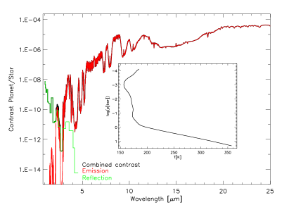
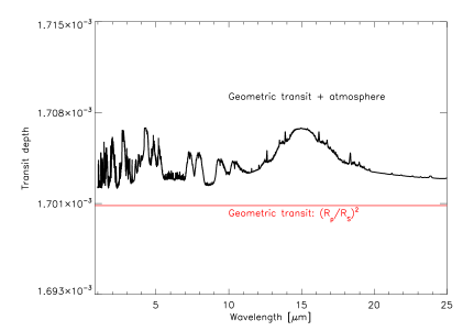
Abbildung 1: Spectra of the 20 bar high-CO₂ case. Left: Secondary eclipse spectrum. Inlet shows the corresponding temperature-pressure profile. Right: Transit depth spectrum.

The line-by-line code MIRART-SQuIRRL (Schreier & Böttger 2003) was used for the calculation of high-resolution synthetic planetary emission, brightness temperature and transmission spectra. Note that the collision-induced absorption (CIA) of CO₂ is not included here, although the CIA is thought to be important in some spectral regions around 7 $\mu$m and longwards of 20 $\mu$m (e.g., Wordsworth et al. 2010a).
Furthermore, the output of the stellar radiative transfer code of the climate model (see above) was used to produce reflection spectra $I_{R}$:

$$I_{R}=\frac{A_{S}}{2}\cdot I_{S}\cdot\frac{R_{s}^{2}}{d^{2}}$$ (1)

where $I_{S}$ is the stellar spectrum, $A_{S}$ the spectral albedo from the stellar radiative transfer code, $R_{s}$ the stellar radius and $d$ the orbital distance. This approach of using the climate model output to construct spectra is based on Kitzmann et al. (2011). A similar method was used by Wordsworth et al. (2011) to calculate synthetic broadband emission spectra of GL 581 d model atmospheres.

These spectra were then used to calculate contrast spectra (i.e., emission + reflection) as well as spectra of effective tangent height of the atmosphere. Calculations in our work closely follow Rauer et al. (2011) where more details can be found. The spectra were calculated on an equidistant spectral grid (in wavenumber), hence the spectral resolution $R$ varies between $R\approx$2-10$\cdot$10³, depending on wavelength.

For a detection of a spectroscopic feature, the relevant quantity is the signal-to-noise ratio (SNR). In contrast to the SNR calculations by, e.g., Kaltenegger & Traub (2009) or Rauer et al. (2011), we take into account not only the stellar photon noise, but also the thermal emission of the telescope, the zodiacal emission and the dark noise. The spectrum of GL 581 used in the SNR calculations is the synthetic spectrum described above. We base our telescope parameters on the James Webb Space Telescope (JWST), assuming a 6.5 m aperture and a detection efficiency of 0.15 (Kaltenegger & Traub 2009). More details on the noise estimates can be found in the Appendix A. The fictitious transit duration of GL 581 d, hence the assumed integration time, is calculated to be 4.15 hours. SNRs are calculated for a spectral resolution of $R$=10, which is a reasonable value in the context of exoplanet characterization.

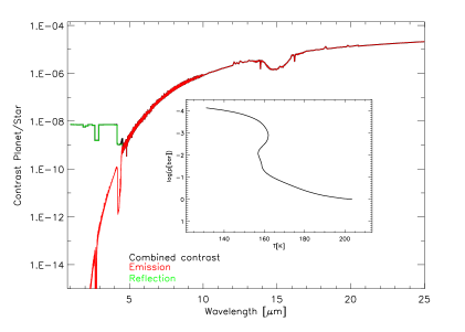
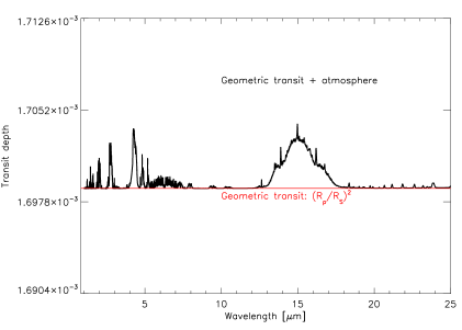
Abbildung 2: Same as Fig. 1, but for the 1 bar low-CO₂ case.

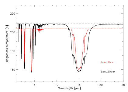
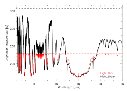
Abbildung 3: Brightness temperature spectra (based on planetary emission only) of the 1 and 20 bar scenarios. Left: Low-CO₂ case. Right: High-CO₂ case. Surface temperatures are indicated by horizontal dashed lines.

4 Results and discussion

4.1 Presence of an atmosphere

The left part of Fig. 1 shows the contrast spectrum of the high-CO₂ 20 bar case. It is clearly seen that the reflection component dominates the near-IR up to about 2.5 $\mu$m and in the window between 3-4 $\mu$m . For longer wavelengths, the emission of the planet is the main component. The broad water and CO₂ absorption bands are clearly seen in the spectrum. Hence, the existence of an atmosphere as well as the presence of water and CO₂ could be inferred. Interestingly, the planet-star contrast is rather low, even though GL 581 is an M-type star and GL 581 d a Super-Earth. The contrast reaches about 4$\cdot$10^-5 in the mid-IR which is about an order of magnitude higher than the contrast between Earth and the Sun. However, it is about 100 times lower than corresponding values for hot Jupiters. The right part of Fig. 1 shows the synthetic transit depth spectrum for the 20 bar high-CO₂ case. It can be seen that due to the presence of large amounts of water and CO₂, the planet appears larger than its geometric radius at all IR wavelengths. Hence, the presence of an atmosphere could also be clearly inferred from transmission spectra due to the wavelength-dependent apparent radius.

Figure 2 also shows contrast and transit spectra, but for the 1 bar low-CO₂ case. The spectra are relatively flat, except for the strong CO₂ fundamental bands. In these bands, the presence of an atmosphere could be inferred, as for the 20 bar high-CO₂ case. Since the atmosphere is very dry (partial pressure of water less than 10^-5 bar), the water bands are difficult to discern in the emission spectrum. In contrast to the high-CO₂ 20 bar case, the secondary eclipse spectrum of the low-CO₂ 1 bar case is dominated by the reflection component up to 4.5 $\mu$m, i.e. the limit of the stellar radiative transfer code of the atmospheric model.

4.2 Atmospheric characterization

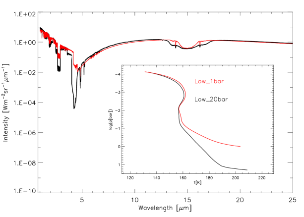
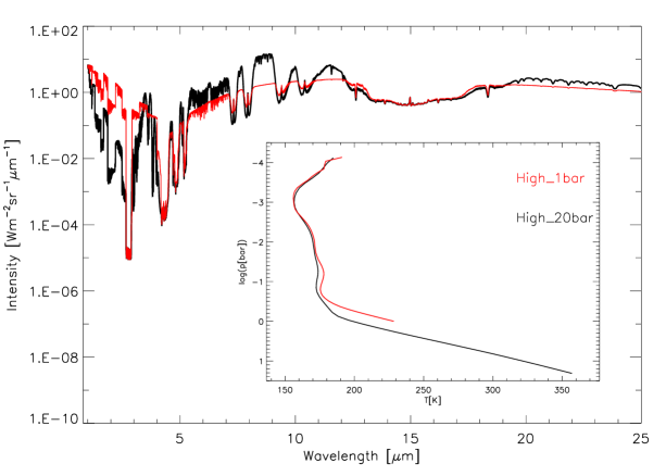
Abbildung 4: Comparison of secondary eclipse spectra of different scenarios: Pressure effect. Scenarios as indicated. Inlet shows the corresponding temperature-pressure profiles.

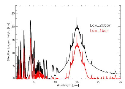
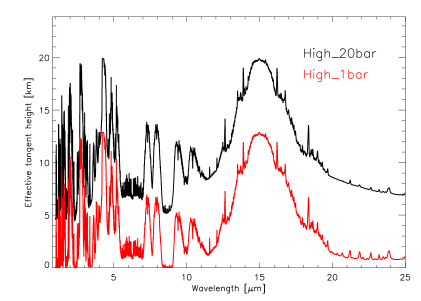
Abbildung 5: Transmission spectra: Pressure effect. Low-CO₂ (left) and high-CO₂ (right).

After securely detecting the atmosphere, the next step would be its characterization (i.e., composition, surface pressure) and, from there, assessing the surface conditions, hence potential habitability.

4.2.1 Surface temperature

Figure 3 shows the brightness temperature spectra of the 1 and 20 bar scenarios of the low-CO₂ (left) and the high-CO₂ case (right). Note that brightness temperature spectra are based only on the emission spectrum since brightness temperatures calculated from the contrast due to the reflection spectrum would yield values up to about 700 K (near 1 $\mu$m). Therefore, characterization of atmospheric temperatures of terrestrial planets is not possible in the near-IR up to about 4-5 $\mu$m.
The left part of Fig. 3 shows that for the low-CO₂ scenarios, the surface temperature could be inferred from the brightness temperature spectra since the atmosphere is transparent except in the CO₂ fundamental bands. By contrast, as can be seen in the right part of Fig. 3, the difference between the brightness temperature and the surface temperature is always non-zero in the high-CO₂ 20 bar case. This means that the emission spectrum does not allow for a determination of the surface temperature, hence to assess potential habitability. The reason for this is that the atmosphere is optically thick for thermal radiation due to the large amounts of CO₂ and water in the atmosphere (von Paris et al. 2010). In the 1 bar high-CO₂ case, some spectral windows would still allow for the determination of the surface temperature which is mostly due to the fact that the atmosphere is much drier than in the high-CO₂ 20 bar case.

4.2.2 Surface pressure

In Fig. 4, the 1 and 20 bar runs with high and low CO₂ concentrations are compared to each other to illustrate how surface pressures could be inferred from secondary eclipse spectra. In the low-CO₂ case (left), the main effect can be seen in the 15 $\mu$m band, which is considerably broader for the 20 bar run than for the 1 bar run. This is simply due to the fact that the line center becomes optically thick at pressures of about 100 mbar, whereas the line wings are transparent up to pressures of the order of 5-10 bar. Also, the 2.7 and 4.3 $\mu$m bands are much deeper in the 20 bar scenario compared to the 1 bar scenario. In the high-CO₂ case (right), the pressure effect in the 15 $\mu$m CO₂ band is much less pronounced. Line wings are already saturated at pressures well below 1 bar. Due to the large difference in surface temperature (see inlet), some spectral regions (e.g., windows near 8-9 $\mu$m or around 11 $\mu$m) differ considerably. Furthermore, in the near-IR, the reflection spectra show large differences, owing to the strong decrease of the spectral albedo with surface pressure. This demonstrates the use of near-IR secondary eclipse measurements for determining atmospheric characteristics besides temperature.

Figure 5 shows the effect of changing surface pressure on the transmission spectrum for the low and the high-CO₂ 1 and 20 bar cases. The spectra show significant differences. For example, in the 9.5 $\mu$m CO₂ band, tangent heights differ by about a factor of 2 to 3. However, in terms of absolute height, this amounts to 5-10 km at most. Note that the CO₂ bands at 7-10 $\mu$m are visible already in the spectra of the high-pressure low-CO₂ scenarios, contrary to the emission spectra where these bands did not appear (see Fig. 4).

These results imply that transmission spectra are in general more sensitive to surface pressure than emission spectra for the cases studied. This is due to two main reasons. Firstly, the tangent height to first order depends on the atmospheric scale height, $H\sim$ $T/m_{a}$ ($T$ is the surface temperature and $m_{a}$ the mean molecular weight of the atmosphere). Thus, for higher surface pressures, and corresponding higher surface temperatures, scale heights are larger. Secondly, for higher surface pressures, atmospheres extend further out to space. For example, the 20 bar high-CO₂ case has its model lid (corresponding to a pressure of 6.6$\cdot$10^-5 bar) at 20 km, whereas the 1 bar case has its model lid at 13 km altitude, which corresponds roughly to 3 scale heights difference.

4.2.3 Surface albedo

The reflectivity of the surface, the surface albedo, is an important parameter to distinguish between different types of surfaces, such as oceans or ice. Reflection spectra could in principle reveal information about the value of the surface albedo.
However, for optically thick atmospheres, as already discussed above, the reflection spectrum does not yield information on the surface albedo in the high-CO₂ 20 bar case. Without the influence of the atmosphere, the reflection contrast would be 7.1 $\cdot$10^-9 (with a fixed surface albedo of $A_{\rm{surf}}$=0.13, see Sect. 3.2). As can be seen from Fig. 1, the reflection contrast is far lower than this value, indicating that even cloud-free atmospheres could inhibit surface characterization via reflection spectra. The same is true for the high-CO₂ 1 bar and the low-CO₂ 20 bar cases (not shown). Only in the low-CO₂ 1 bar case, the reflection spectrum would allow to infer the surface albedo (see Fig. 2).

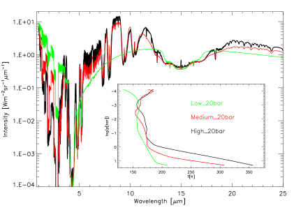
Abbildung 6: Comparison of secondary eclipse spectra of different scenarios: Concentration effect. Inlet shows the used temperature-pressure profiles.

4.2.4 Atmospheric composition

Fig. 6 shows secondary eclipse spectra at equal surface pressures (20 bar), but for different CO₂ concentrations (high, medium, low). It is rather difficult to distinguish between the medium and high-CO₂ scenario, except for some narrow spectral windows. When comparing Fig. 4 with Fig. 6, it is therefore difficult to decide whether the shape of the spectrum is actually due to a pressure difference at high CO₂ concentration or a concentration difference at high surface pressures. It is, however, possible to distinguish between high or low CO₂ concentrations by the presence of many weak CO₂ bands in the high-CO₂ case, e.g. at around 7, 9 and 10 $\mu$m. These bands do not appear in the spectrum unless CO₂ concentrations exceed several percent. Additionally, the presence of water can be inferred from the strong 6.3 $\mu$m fundamental band and the signatures of the rotation band in the mid- to far-IR. Thus, dry and moist atmospheres could be distinguished.

In order to show the effect of changing CO₂ concentration on transmission spectra, Fig. 7 compares the 20 bar scenarios for low, medium and high CO₂ concentrations. Interestingly, the medium-CO₂ case shows a more pronounced 15 $\mu$m band of CO₂ despite the fact that the high-CO₂ scenario is significantly warmer at the surface (by about $\sim$ 40 K). This is due to the lower mean atmospheric molecular mass (hence, higher scale height) which is $\sim$ 29 g mol^-1 in the medium-CO₂ case and $\sim$ 43 g mol^-1 in the high-CO₂ case. The weak bands around 7 and 10 $\mu$m do not differ by much. Still, in the water rotation bands (longwards of 20 $\mu$m) and the strong CO₂ fundamentals, rather large differences in the spectrum can be seen. This indicates that transmission spectroscopy could be able to distinguish between different CO₂ concentrations.

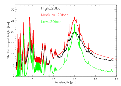
Abbildung 7: Transmission spectra: Concentration effect.

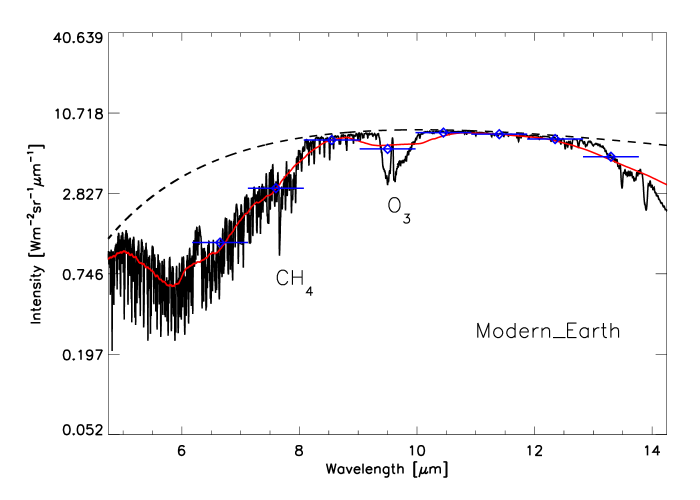
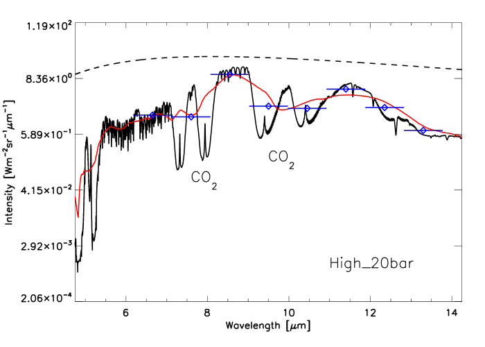
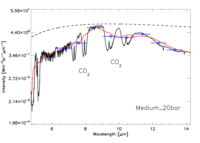
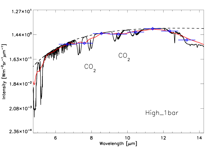
Abbildung 8: Possibility of a false-positive biomarker detection for different scenarios, as indicated. Modern Earth spectrum taken from Grenfell et al. (2011). Planck curves of corresponding surface temperatures as dashed lines. Smoothed (red) and binned spectra (blue) are for a spectral resolution of 10.

The same is true for the comparison of low and high-CO₂ scenarios. Here, however, the differences in the spectrum are visible in the weak bands of CO₂ (e.g., around 10 $\mu$m) rather than in the strong fundamentals (4.3 and 15 $\mu$m).

4.2.5 Surface conditions

In summary, the characterization of surface conditions on GL 581 d by secondary eclipse spectroscopy would be rather difficult, even if the planet were to be transiting. It would be possible to approximately constrain CO₂ and water concentrations in the atmosphere, however, constraining surface pressures or surface temperatures, hence assess habitability, is complicated by degeneracies, as stated above. Overall, results imply that it is easier to characterize the atmospheric scenarios of GL 581 d with transmission spectroscopy than with emission spectroscopy, especially with respect to the habitable scenarios with massive CO₂ atmospheres. However, surface pressures cannot be inferred directly with transmission spectra since effective tangent heights are always of the order of a few kilometres. Still, when combining several spectral bands and using both transmission and emission spectra, it may be possible to constrain the surface pressure as well as CO₂ concentrations and the presence of water. Thus, in principle, through atmospheric modeling surface conditions could be assessed.

4.3 Biomarkers

Although the model scenarios used in this work only consider H₂O-CO₂-N₂ atmospheres, we can compare the computed spectra with spectral signatures of modern Earth to discuss the potential for false-positive or false-negative identifications of biomarkers.

4.3.1 False-positive detections of biomarkers

As an illustration, Fig. 8 shows high-resolution and binned (with $R$=10) emission spectra of GL 581 d in comparison to modern Earth. The modern Earth spectrum (taken from Grenfell et al. 2011) is shown in the upper left, the GL 581 d scenarios from this work are (clockwise) high-CO₂ 20 bar, high-CO₂ 1 bar and the medium-CO₂ 20 bar case. The spectra are centered around 9.6 $\mu$m which is the position of the main absorption band of ozone. This absorption feature is close to an absorption band of CO₂ at around 9.5 $\mu$m which is clearly seen in all GL 581 d spectra in Fig. 8.

Additionally indicated is the position of the 7.7 $\mu$m band of methane (overlapping the 7.8 $\mu$m band of nitrous oxide) which again is close to absorption bands of CO₂ at 7.5 and 8 $\mu$m. The methane band is hardly discernible in the Earth spectrum, at the considered resolution of $R$=10. However, in the GL 581 d scenarios shown in Fig. 8, an absorption is seen, which in this case is due to CO₂. These CO₂ bands at biomarker positions (7.5, 8, 9.5 $\mu$m) are also present in the transmission spectra (e.g., Fig. 7), implying that transmission spectra also suffer from the possibility of false-positive biomarker detections.

At this low spectral resolution, the spectral features around 9.6 $\mu$m, due to CO₂ in the GL 581 d cases or due to ozone in the Earth case, look similar. Thus, the CO₂ bands could be mistaken for actual biomarker signals, at the expected low spectral resolution used for exoplanet characterization. This is the case for the emission spectra of medium and high-CO₂ scenarios, whereas in the low-CO₂ case (not shown in this Fig.), the respective CO₂ bands are too weak to produce false detections. In the transmission spectra (e.g., Fig. 7), these bands also appeared for high-pressure, low-CO₂ scenarios which implies that false-positives are possible in transmission spectra even for these scenarios.

One possible way of avoiding such false-positive detections in the cases presented here (i.e., CO₂-rich atmospheres) is to exploit the double nature of the CO₂ bands around 7 and 10 $\mu$m. If spectral observations are performed, e.g., at 9.5 and 10.5 $\mu$m, and both filters show a deep absorption, then the spectral signatures are most likely due to CO₂. Hence, a possible spectral characterization with respect to biomarkers should be done in all main IR CO₂ bands (2-15 $\mu$m) in order to avoid false-positive detections.

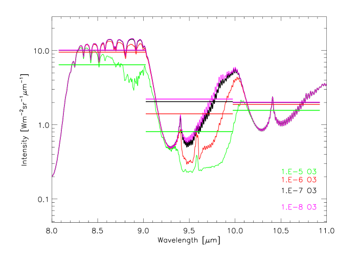
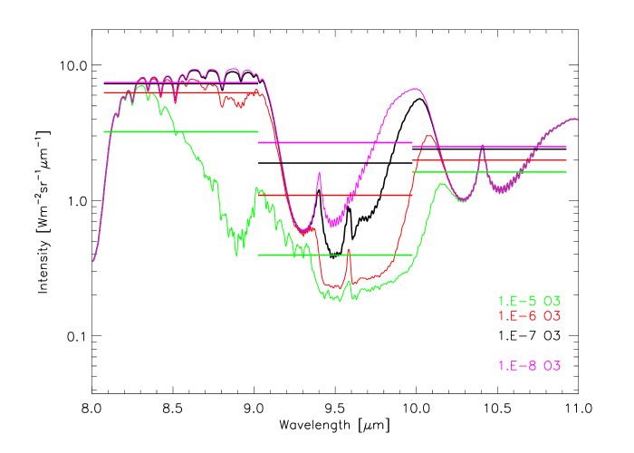
Abbildung 9: Effect of O₃ isoprofiles on emission spectra. Constant O₃ concentrations as indicated. Left: High-CO₂ 20 bar, right: Medium-CO₂ 20 bar. Horizontal lines represent binned spectra for a spectral resolution of 10.

4.3.2 False-negative detection of biomarkers

In order to investigate the possibility of false-negative detections of ozone, we calculated model spectra of the high-CO₂ 20 bar case and of the medium-CO₂ 20 bar case where we additionally introduced artificial profiles of ozone in the line-by-line spectral calculations. These ozone profiles have not been implemented in the 1D climate calculations. However, they are not expected to strongly influence the temperature structure of the atmosphere (e.g., Kaltenegger et al. 2011) because of the lack of UV radiation emitted by GL 581 in the wavelength regime where ozone heating occurs.
In a first attempt, we used isoprofiles of ozone in the calculation of the spectra. Chosen concentrations were 10^-8, 10^-7, 10^-6 and 10^-5, respectively. This choice of concentrations broadly covers the range of ozone concentrations found in the present Earth atmosphere (10^-8 near the surface, about to almost 10^-5 in the mid-stratosphere).
Results of this sensitivity analysis are shown in Fig. 9 for the high-CO₂ and medium-CO₂ 20 bar cases. Clearly, a detection of ozone at low concentrations of 10^-8 or 10^-7 would not be possible at low spectral resolution. For the high-CO₂ 20 bar case, even a concentration of 10^-6 would be very challenging to detect. In both cases shown here, however, it would be possible to infer ozone levels of 10^-5 since the calculated intensity drops by about a factor of 3-8 in the center of the ozone fundamental band.

In reality, ozone profiles will most likely not be in the form of isoprofiles. The production of ozone proceeds through the three-body reaction

$$O_{2}+O+M\rightarrow O_{3}+M$$ (2)

where $M$ is, on Earth, typically nitrogen. The production of the atomic oxygen needed in eq. 2 requires photolysis of molecular oxygen, carbon dioxide or water. Hence, there is a trade-off between the necessary UV radiation for photolysis and the density to enable the three-body production reaction, which is why photochemical models generally predict a distinct maximum of atmospheric ozone concentrations around the 1-10 millibar pressure range.
The actual location of this ozone maximum depends on the stellar UV radiation field, the ozone and the oxygen content of the atmosphere (Selsis et al. 2002, Segura et al. 2003, Segura et al. 2007, Domagal-Goldman & Meadows 2010, Grenfell et al. 2011). Therefore, we inserted artificial ozone profiles $C_{O_{3}}$ as a function of pressure $p$ based on a Gaussian profile

$$C_{O_{3}}\left(p\right)=C_{\rm{max}}\cdot exp\left(-\frac{\left(log\frac{p}{p_{m}}\right)^{2}}{0.5}\right)$$ (3)

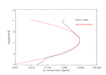
Abbildung 10: Modern Earth mean ozone profile from Grenfell et al. (2011) and approximation (in red) with eq. 3 using $C_{\rm{max}}$=9ppm and $p_{m}$=6 mbar.

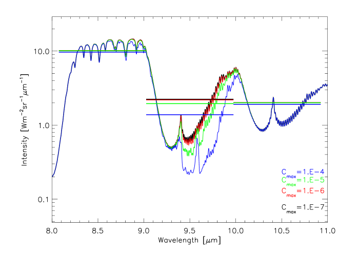
Abbildung 11: Effect of O₃ profiles on emission spectra. Parameters for eq. 3: $C_{\rm{max}}$ as indicated, $p_{m}$=10mbar. Left: High-CO₂ 20 bar, right: Medium-CO₂ 20 bar. Horizontal lines represent binned spectra for a spectral resolution of 10.

where $C_{\rm{max}}$ is the maximum ozone concentration reached at pressure $p_{m}$. Fig. 10 shows the approximation of an Earth ozone profile with eq. 3. The agreement near the maximum of the ozone layer is rather good.
Figure 11 shows the effect of varying $C_{\rm{max}}$ on emission spectra at constant $p_{m}$ of 10 mbar. Shown are the spectra for the high-CO₂ and medium-CO₂ 20 bar cases. In Fig. 12, the effect of varying $p_{m}$ on the spectrum at constant $C_{\rm{max}}$ of 10 ppm is illustrated for the high-CO₂ 20 bar case.
Note that tropospheric concentration maxima, i.e. at pressures higher than 100 mbar, are usually not expected from atmospheric chemistry modeling. Rather, maxima are found in the lower to upper stratosphere. Hence the scenarios with $p_{m}$ of 100 or 1,000 mbar shown in Fig. 12 are most likely overestimating the ozone column.
From Fig. 11, it is evident that it is very difficult to infer the presence of ozone even at high concentrations of about 10 ppm. Only for the profile with $C_{\rm{max}}$=100ppm, it would be possible to detect an additional absorption besides the CO₂ band.
Figure 12 shows that for a value of $p_{m}$=100mbar or higher, it would be possible to detect ozone in the spectrum. However, as stated above, such a tropospheric maximum of ozone is not very probable.

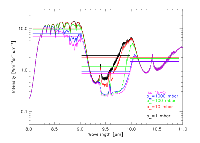
Abbildung 12: Effect of maximum of O₃ profiles on emission spectra for the high-CO₂ 20 bar case. Parameters for eq. 3: $C_{\rm{max}}$=10ppm, $p_{m}$ in mbar as indicated. Horizontal lines represent binned spectra for a spectral resolution of 10.

These sensitivity studies illustrate that an inferred absence of ozone could be possible for the atmospheric scenarios considered in this work, even if ozone would be present in large concentrations of the order of 10^-6-10^-5. Hence, also the possibility of false-negatives of ozone needs to be taken into account when investigating CO₂-rich, potentially habitable atmospheric scenarios.

4.4 Detectability

Tabelle 2: SNR values for secondary eclipse spectroscopy. Telescope configuration JWST, integration time 4.15 hours, spectral resolution R=10.

Scenario	8.5 $\mu$m	9.5 $\mu$m	11.5 $\mu$m	15 $\mu$m	20 $\mu$m
low-CO2 1 bar	0.050	0.091	0.19	0.10	0.23
low-CO2 20 bar	0.062	0.10	0.22	0.088	0.25
medium-CO2 1 bar	0.064	0.10	0.22	0.091	0.26
medium-CO2 20 bar	0.56	0.28	0.51	0.089	0.34
high-CO2 1 bar	0.12	0.15	0.37	0.10	0.34
high-CO2 20 bar	0.77	0.22	0.74	0.10	0.48

Tabelle 3: SNR values for transmission spectroscopy. Telescope configuration JWST, integration time 4.15 hours, spectral resolution R=10.

Scenario	2.0 $\mu$m	2.7 $\mu$m	4.3 $\mu$m	6.3 $\mu$m	7.7 $\mu$m	9.5 $\mu$m	15 $\mu$m
low-CO2 1 bar	0.41	0.65	0.83	0.091	0.027	8.4 10-3	0.21
low-CO2 20 bar	1.1	1.2	1.4	0.24	0.22	0.12	0.33
medium-CO2 1 bar	1.0	1.1	1.2	0.12	0.23	0.12	0.29
medium-CO2 20 bar	2.1	1.9	2.0	0.46	0.65	0.46	0.44
high-CO2 1 bar	0.96	0.89	0.94	0.10	0.26	0.15	0.22
high-CO2 20 bar	1.9	1.6	1.6	0.50	0.65	0.46	0.35

The main spectral bands investigated for detectability are the 2.0, 2.7, 4.3, 7.7, 9.5 and 15 $\mu$m CO₂ absorption bands as well as the 6.3 $\mu$m H₂O absorption band in transmission. For secondary eclipse spectroscopy, only the 9.5 and 15 $\mu$m CO₂ and the 20 $\mu$m H₂O bands were considered. Additionally two filters outside of broad absorption bands are calculated, namely at 8.5 and at 11.5 $\mu$m. These two filters offer the possibility to characterize surface temperatures in optically thin atmospheres.
Furthermore, six representative scenarios are considered, namely the 1 and 20 bar runs of the low, medium and high-CO₂ cases.

Table 2 summarizes the SNR values for secondary eclipse spectroscopy. It is clearly seen that, even though GL 581 is a very close star (6.27 pc, Butler et al. 2006), obtainable SNR values are very small, only reaching values of 0.3-0.77. The reason for the low SNR values in the mid- to far IR is the effect of the zodiacal background chosen here (see Appendix A) which reduces SNR values by about a factor of 5 at 20 $\mu$m and a factor of 2 at 15 $\mu$m compared to the photon-limited case. A similar result was already found by, e.g., Belu et al. (2011).

Table 3 summarizes the SNR values for transmission spectroscopy. SNR values are mostly below unity. The exceptions are the 2.0, 2.7 and 4.3 $\mu$m near-IR fundamentals of CO₂. In these bands, characterization of the GL 581 d scenarios, as outlined above, could be feasible. A clear distinction between, e.g., high and low-CO₂ cases is still very difficult, given that the SNR values are only marginally larger than unity. One strategy to obtain larger SNRs is the co-adding of transits. This might result in a significant increase of the SNR since the SNR scales with the square root of the number of transits. Assuming a 5-year mission lifetime of JWST (3-4 transits observable per year) would lead to SNRs of about a factor of 4 higher compared to the values shown in Tables 2 and 3.

5 Conclusions

We presented synthetic emission and transmission spectra for a wide range of atmospheric scenarios of the potentially habitable Super-Earth GL 581 d. These spectra were used as an example of possible future spectroscopic investigations of candidate habitable planets.

Water and carbon dioxide could be clearly seen in the calculated spectra due to prominent absorption bands, indicating the presence of an atmosphere.

The determination of surface temperatures was possible for model atmospheres with either low surface pressures or low CO₂ content. The potentially habitable, CO₂-rich scenarios did not allow for the characterization of surface temperatures. Thus, their potential habitability could not be assessed directly from the spectra, in agreement with a model spectrum from Kaltenegger et al. (2011). The further determination of atmospheric conditions was complicated by degeneracies between the surface pressure and the CO₂ concentration. However, when combining observations in several spectral bands and using both transmission and emission spectra, inferring approximative CO₂ concentrations and surface pressures would be possible.

With currently planned telescope designs such as JWST, SNR values for emission and transmission spectroscopy are, however, rather low, implying that the detection of an atmosphere of a ”GL 581 d-liketransiting planet is challenging. Reasonable, single-transit SNR could only be calculated for three near-IR CO₂ fundamentals at 2.0, 2.7 and 4.3 $\mu$m (transmission spectroscopy). In the mid- to far-IR, thermal and zodiacal background noises inhibit SNRs above unity.

Results indicate that the search for biomarkers in CO₂-rich or high-pressure atmospheres would suffer from the possibility of false-positive detections, in agreement with previous studies (e.g., Schindler & Kasting 2000 or Selsis et al. 2002). This is due to absorption bands of CO₂ which occur close to main biomarker absorption bands. However, if the main CO₂ IR bands were to be observed simultaneously, such false-positive detections could possibly be avoided. This will be subject of future modeling including Earth-like atmospheric composition. Results also imply that CO₂ absorption bands could mask the spectroscopic features of ozone, hence produce false-negative detections. This was shown to be possible even if ozone would be present in rather large concentrations of up to 10^-5.

Anhang A Noise contributions

The total SNR $S_{p}$ of a planetary feature is calculated with

$$S_{p}=\frac{F_{p}}{\sigma_{\rm{total}}}$$ (4)

where $F_{p}$ is the planetary signal measured during secondary eclipse (emitted and reflected spectrum) or primary eclipse (additional transit depth due to atmospheric absorption). $\sigma_{\rm{total}}$ represents the total noise of the measurement. In addition to the stellar noise $\sigma_{S}$, main contributions to the noise budget come from the zodiacal emission of the solar system (denoted $\sigma_{\rm{zodi}}$), the thermal emission of the mirror and, in the case of the JWST, the sun shade (denoted $\sigma_{\rm{thermal}}$). Both components need to be taken into account in the SNR calculations since their effect on detectability could be significant, especially in the mid-IR, longwards of 10 $\mu$m (e.g., Deming et al. 2009, Belu et al. 2011). In addition, the dark noise $\sigma_{d}$ is considered here. Hence, we have

$$\sigma_{\rm{total}}=\sqrt{2\cdot(\sigma_{S}^{2}+\sigma^{2}_{\rm{thermal}}+\sigma^{2}_{\rm{zodi}}+\sigma_{d}^{2})}$$ (5)

The thermal noise was obtained from

$$\sigma_{\rm{thermal}}^{2}=q_{e}\cdot\epsilon\cdot B_{\lambda}(T_{\rm{JWST}})\cdot t_{t}\cdot n_{\rm{px}}\cdot S_{A}\cdot A_{E}\cdot\frac{\lambda}{R}$$ (6)

where $\epsilon$ is the emissivity, $B_{\lambda}(T_{\rm{JWST}})$ the blackbody emission of the telescope and sun shade, $t_{t}$ the integration time (here assumed to be the transit duration, i.e. 4.15 hours), $n_{\rm{px}}$ the number of pixels used for the integration on the detector, $\lambda$ the considered wavelength and $R$ the spectral resolution, $A_{E}$ the emitting area, $q_{e}$=0.15 the quantum efficiency of the telescope (e.g., Kaltenegger & Traub 2009, Rauer et al. 2011) and $S_{A}$ the solid angle per pixel.
We assumed a telescope and sun shade temperature $T_{\rm{JWST}}$ of 45 K with an emissivity of $\epsilon$=0.15 (Belu et al. 2011) and a total emitting surface of sun shade and mirror combined of $A_{E}$=240 m² (Nella et al. 2002). The number of pixels $n_{\rm{px}}$ is calculated with

$$n_{\rm{px}}=n_{\rm{spatial}}\cdot n_{\rm{spectral}}\cdot\frac{\lambda}{R}$$ (7)

where $n_{\rm{spatial}}$ and $n_{\rm{spectral}}$ the number of pixels in spatial and spectral (per $\mu$m) direction, respectively. We assumed $n_{\rm{spectral}}$=32.33 pixel $\mu$m^-1, mimicking the MIRI instrument in the 5-11 $\mu$m spectral range (Belu et al. 2011). The number of pixels in the spatial direction is obtained from

$$n_{\rm{spatial}}=2.4\cdot\frac{\lambda}{d_{t}\cdot p_{s}}$$ (8)

with $d_{t}$ the telescope diameter (i.e., 6.5 m in the case of JWST) and $p_{s}$=0.11per pixel the instrumental pixel scale. The number calculated from eq. 8 is then rounded up to the closest multiple of 4. The solid angle per pixel is calculated with (1 sq. deg $\approx\frac{1}{3282}$ sr)

$$S_{A}=\frac{p_{s}^{2}}{3600^{2}\cdot 3282}$$ (9)

The zodiacal emission $I_{Z}$ (given in W m^-2 $\mu$m^-1 sr^-1) used in the noise calculations is taken from one example measurement in the ecliptic plane presented by Kelsall et al. (1998) (their Fig. 9). Note that this choice is a rather pessimistic assumption since some potential targets will probably be located towards higher ecliptic latitudes, hence the corresponding zodiacal noise would be somewhat reduced. We calculate the zodiacal noise via

$$\sigma_{\rm{zodi}}^{2}=I_{Z}\cdot n_{\rm{px}}\cdot S_{A}\cdot A_{\rm{tel}}\cdot t_{t}\cdot q_{e}\cdot\frac{\lambda}{R}$$ (10)

with $A_{\rm{tel}}$ the telescope area, assuming a circular aperture of 6.5 m.
The dark noise contribution to the noise budget is calculated from

$$\sigma_{d}^{2}=d_{c}\cdot n_{\rm{px}}\cdot t_{t}$$ (11)

where $d_{c}$=0.03 e^- pixel^-1 s^-1 is the dark current (MIRI, see e.g. Deming et al. 2009 or Belu et al. 2011).