Electromagnetic counterparts from counter-rotating relativistic kicked discs

Abstract

We show the results of two dimensional general relativistic inviscid and isothermal hydrodynamical simulations comparing the behavior of co-rotating (with respect to the black hole rotation) and counter-rotating circumbinary quasi-Keplerian discs in the post merger phase of a supermassive binary black hole system. While confirming the spiral shock generation within the disc due to the combined effects of mass loss and recoil velocity of the black hole, we find that the maximum luminosity of counter-rotating discs is a factor $\sim(2-12)$ higher than in the co-rotating case, depending on the spin of the black hole. On the other hand, the luminosity peak happens $\sim 10$ days later with respect to the co-rotating case. Although the global dynamics of counter-rotating discs in the post merger phase of a merging event is very similar to that for co-rotating discs, an important difference has been found. In fact, increasing the spin of the central black hole produces more luminous co-rotating discs while less luminous counter-rotating ones.

.

1 Introduction

In the last few years a lot of attention has been given to the possibility of detecting the electromagnetic (EM) counterpart of the gravitational wave signal produced in the merger event between two supermassive binary black holes (SMBBHs), whose gravitational waves should be detected by the planned Laser Interferometric Space Antenna (LISA) (see, among the others, Bogdanović et al., 2011; Haiman et al., 2009; Palenzuela et al., 2010; Sesana et al., 2009; Stavridis et al., 2009; Babak et al., 2011).

Our current understanding of the physics of these systems distinguishes between a pre-merger phase and a post-merger phase. The EM emission properties of the pre-merger phase have been studied by several authors, including  Mösta et al. (2010); Bode et al. (2010); Chang et al. (2010); Shapiro (2010); Liu and Shapiro (2010). Chang et al. (2010), in particular, showed that, approximately one day before the merger is completed, there is a late time precursor brightening from tidal and viscous dissipation in the inner disc. On the other hand, the typical behavior of the SMBBH system in the post-merger phase is characterized by two distinct but related physical effects having to do with the emission of gravitational waves, namely an abrupt mass loss and a sudden recoil of the resultant black hole. Observationally, the “recoil event” has recently found indirect confirmation through spectropolarimetric measurements of the quasar E1821+643 (Robinson et al., 2010), that are consistent with a scattering model in which the broad-line region has two components, moving with different bulk velocities away from the observer. The kick velocity and the mass loss of the black hole are extremely relevant both because they represent an imprint of the gravitational wave emission, and because they have strong dynamical effects on the circumbinary disc, whose inner radius is that possessed at the time when the binary in-spiral time scale became shorter than the viscous time scale in the disc.

When investigating the response of the disc to the mass loss of the black hole and its recoil velocity, an additional physical effect that needs to be taken into account is that produced by counter-rotation. The term co-rotation (counter-rotation) has two different meanings when applied to the pre-merger phase, when it has to be intended as rotation in the same (opposite) sense of the merging binary, and when applied to the post-merger phase, when it has to be intended as rotation in the same (opposite) sense of the spinning resultant black hole. It is worth recalling that, on a broader sense, counter-rotating discs are a relatively common phenomenon in galaxies. Coccato et al. (2011) report a list of galaxies, including the well studied case of NGC4550 (Rubin et al., 1992), where two co-spatial stellar discs, one orbiting prograde, the other one orbiting retrograde, have been observed. In general, large scale counter-rotating stellar discs manifest preferentially in early-type spirals, while $20\%$ of the gas discs in S0 galaxies is thought to counter-rotate. As far as SMBBHs systems are concerned, MacFadyen and Milosavljević (2008) speculate about the important dynamical differences that may be present in a counter-rotating disc during the pre-merger phase. Quite recently Nixon et al. (2010) have performed a detailed analysis, both analytical and numerical, of the retrograde accretion in merging supermassive black holes, reaching the conclusion that the binary orbit, by absorbing negative angular momentum from the circumbinary disc via gas capture, may become eccentric. In particular, the binary coalesces once it has absorbed the angular momentum of a gas mass comparable to that of the secondary black hole.

All of these investigations, however, refer to the pre-merger phase. During the post-merger phase, it is not clear whether a retrograde disc may have significant effects on both the dynamics and the EM signal emitted by the system. Several time dependent numerical investigations of prograde circumbinary discs in the post-merger phase have been performed, both in a Newtonian (Lippai et al., 2008; O’Neill et al., 2009; Corrales et al., 2010; Rossi et al., 2010) and in a relativistic framework (Megevand et al., 2009; Anderson et al., 2010; Zanotti et al., 2010). With different emphasis and caveats, the majority of these works have confirmed the possibility of detecting a significant EM counterpart from SMBBHs. By extending the analysis of Zanotti et al. (2010), in this paper the role of retrograde rotation in the post-merger phase is studied through numerical simulations, with the special aim of comparing the emitted luminosity with respect to the prograde rotation case.

The paper is organized as follows. In Section 2 and in Sec. 3 the essential information about the physical properties of the initial models, and about the numerical code adopted in the simulations are provided. Section 4 is devoted to the presentations of the results, while Section 5 contains a summary of the work. A signature $\{-,+,+,+\}$ for the space-time metric is assumed and Greek letters (running from $0$ to $3$) for four-dimensional space-time tensor components are used, while Latin letters (running from $1$ to $3$) will be employed for three-dimensional spatial tensor components. Moreover, $c=G=1$ and the geometric system of units is extended by setting $m_{p}/k_{B}=1$, where $m_{p}$ is the mass of the proton, while $k_{B}$ is the Boltzmann constant. In this way the temperature is a dimensionless quantity.

2 Initial conditions

Table 1: Main properties of the initial models. From left to right the columns report the name of the model, the black hole spin parameter $a$, the power-law index $q$ and the parameter ${\cal S}$ of the angular momentum distribution, the inner and the outer radius of the disc, $r_{\rm in}$ and $r_{\rm out}$, the radius of the maximum rest-mass density $r_{\rm c}$, the orbital period at the radius of maximum rest-mass density $\tau_{\rm c}$, the uniform temperature $T$ assumed during isothermal evolution. The adiabatic index $\gamma=5/3$ and the mass of the black hole is $M=1.0\times 10^{6}M_{\odot}$ in each model.

Model	$J/M^{2}$	$q$	${\cal S}$	$r_{\rm in}$	$r_{\rm out}$	$r_{\rm c}$	$\tau_{\rm c}$	$T$
				$(M)$	$(M)$	$(M)$	$(d)$	$(K)$
CoRot_a.0.1	$0.1$	$0.4955$	$1.033$	$668$	$1998$	$1082$	$12.76$	$2.68\times 10^{6}$
CoRot_a.0.5	$0.5$	$0.4955$	$1.033$	$598$	$2138$	$1036$	$11.95$	$2.68\times 10^{6}$
CoRot_a.0.9	$0.9$	$0.4955$	$1.033$	$537$	$2273$	$988$	$11.13$	$2.68\times 10^{6}$
CoRot_a.0.99	$0.99$	$0.4955$	$1.033$	$524$	$2303$	$977$	$10.94$	$2.68\times 10^{6}$
CounterRot_a.0.1	$0.1$	$0.4955$	$-1.034$	$534$	$3270$	$1104$	$13.15$	$2.68\times 10^{6}$
CounterRot_a.0.5	$0.5$	$0.4955$	$-1.034$	$577$	$3144$	$1149$	$13.95$	$2.68\times 10^{6}$
CounterRot_a.0.9	$0.9$	$0.4955$	$-1.034$	$622$	$3019$	$1192$	$14.75$	$2.68\times 10^{6}$
CounterRot_a.0.99	$0.99$	$0.4955$	$-1.034$	$633$	$2991$	$1202$	$14.93$	$2.68\times 10^{6}$
CounterRot_T1	$0.9$	$0.4955$	$-1.034$	$622$	$3019$	$1192$	$14.75$	$4.47\times 10^{5}$
CounterRot_T2	$0.9$	$0.4955$	$-1.034$	$622$	$3019$	$1192$	$14.75$	$8.94\times 10^{5}$
CounterRot_T3	$0.9$	$0.4955$	$-1.034$	$622$	$3019$	$1192$	$14.75$	$8.05\times 10^{6}$
CounterRot_T4	$0.9$	$0.4955$	$-1.034$	$622$	$3019$	$1192$	$14.75$	$1.61\times 10^{7}$

The initial model is given by a stationary and axisymmetric configuration obtained after solving the relativistic Euler equations in the fixed background spacetime of a Kerr black hole. Such solution is due to Kozlowski et al. (1978) while a detailed description for computing the corresponding equilibrium models can be found in Daigne and Font (2004). The specific angular momentum of the resulting geometrically thick disc obeys a power law on the equatorial plane, namely $\ell(r,\theta=\pi/2)={\cal S}r^{q}$, where ${\cal S}$ is positive or negative, corresponding to a disc rotation that is prograde or retrograde with respect to the black hole rotation. Table 1 reports the main parameters of the models considered, differing for the rotation law, for the spin of the central black hole, and for the temperature of the disc. Having chosen the exponent $q$ to be close to $1/2$ in all of the models, the rotation law tends to the Keplerian one, and the disc flattens towards the equatorial plane, thus making its vertical structure negligible. The equation of state of the initial model is that of a polytrope $p=\kappa\rho^{\gamma}$, with $\gamma=5/3$. It should be noted that it is not possible to build two models, one co-rotating and the other one counter-rotating, while maintaining all of the other physical parameters unmodified. In particular, a specific counter-rotating model is larger than the corresponding co-rotating model with the same disc temperature. Another relevant difference among the two classes of models, which is clearly visible by inspection of Table 1, is that, while for co-rotating models the radius of the maximum rest mass density decreases for larger spins of the central black hole, the opposite happens for counter-rotating models. This will have important implications on the dependence of the emitted luminosity on the spin, as discussed in Sec. 4.

The recoil effect on the black hole resulting from a SMBBHs merger was predicted well before (Bekenstein, 1973; Redmount and Rees, 1989) numerical relativistic simulations were able to prove its existence and measure its magnitude. Because in this contribution only two dimensional simulations are performed, the recoil velocity vector has to lie on the orbital plane of the disc, which is consistent with a binary merger between two black holes having the same mass and with spins that are equal in modulus and both perpendicular to the orbital angular momentum (Campanelli et al., 2007; Rezzolla, 2009). Since the recoil velocities in the orbital plane are expected to be $\lesssim 450\,\rm{km}/\rm{s}$ (Koppitz et al., 2007; Herrmann et al., 2007; Pollney et al., 2007), the conservative value $V_{\rm k}=300\,\rm{km}/\rm{s}$ is adopted. In order to simulate this effect numerically, at time $t=0$ a Lorentz boost to the fluid velocity of the disc is applied, oriented along the radial direction with $\phi=0$. In addition, $2\%$ of the total mass-energy of the merged black hole is assumed to be radiated away in gravitational waves. In practice, the initial model is first computed in the gravitational potential of the full black hole mass, and then evolved in the gravitational potential of the reduced mass.

3 Numerical method

The equations of general relativistic hydrodynamics are solved in the stationary spacetime of a Kerr black hole, written in Boyer-Lindquist coordinates, through the ECHO code (Del Zanna et al., 2007). ECHO adopts a $3+1$ split of spacetime in which the space-time metric is decomposed according to

$$\mathrm{d}s^{2}=g_{\mu\nu}dx^{\mu}dx^{\nu}=\!-\alpha^{2}\mathrm{d}t^{2}+\gamma_{ij}\,(\mathrm{d}x^{i}\!+\beta^{i}\mathrm{d}t)(\mathrm{d}x^{j}\!+\beta^{j}\mathrm{d}t),$$ (1)

where $\alpha$ is the lapse function, $\beta^{i}$ is the shift vector, and $\gamma_{ij}$ is the spatial metric tensor, with $i$ and $j$ running from $1$ to $3$. Moreover, ECHO adopts a conservative formulation of the general-relativistic inviscid hydrodynamical equations, by solving the system

$$\partial_{t}\vec{\mathcal{U}}+\partial_{i}\vec{\mathcal{F}}^{i}=\vec{\mathcal{S}},$$ (2)

where the vector of conservative variables $\vec{\mathcal{U}}$ and the corresponding fluxes $\vec{\mathcal{F}}^{i}$ in the $i$ direction are respectively given by

$$\vec{\mathcal{U}}\equiv\sqrt{\gamma}\left[\begin{array}[]{c}D\\ \\ S_{j}\\ \\ U\end{array}\right],~{}~{}~{}\vec{\mathcal{F}}^{i}\equiv\sqrt{\gamma}\left[\begin{array}[]{c}\alpha v^{i}D-\beta^{i}D\\ \\ \alpha W^{i}_{j}-\beta^{i}S_{j}\\ \\ \alpha S^{i}-\beta^{i}U\end{array}\right],$$ (3)

whereas the sources, in any stationary background metric, can be written as

$$\vec{\mathcal{S}}\equiv\sqrt{\gamma}\left[\begin{array}[]{c}0\\ \\ \frac{1}{2}\alpha W^{ik}\partial_{j}\gamma_{ik}+S_{i}\partial_{j}\beta^{i}-U\partial_{j}\alpha\\ \\ \frac{1}{2}W^{ik}\beta^{j}\partial_{j}\gamma_{ik}+{W_{i}}^{j}\partial_{j}\beta^{i}-S^{j}\partial_{j}\alpha\end{array}\right]\ .$$ (4)

The determinant of the spatial metric $\sqrt{\gamma}$ and of the global metric $\sqrt{-g}$ are related by $\sqrt{\gamma}\equiv\sqrt{-g}/\alpha$. The conservative variables $(D,S_{j},U)$ that are evolved by the numerical scheme are related to the rest-mass density $\rho$, to the thermal pressure $p$ and to the fluid velocity $v_{i}$ by

$$D\equiv\rho W,$$ (5)

$$S_{i}\equiv\rho hW^{2}v_{i},$$ (6)

$$U\equiv\rho hW^{2}-p,$$ (7)

where $W=(1-v^{2})^{-1/2}$ is the Lorentz factor of the fluid with respect to the Eulerian observer associated to the $3+1$ splitting of the spacetime, and

$$W_{ij}\equiv\rho hW^{2}v_{i}v_{j}+p\gamma_{ij}\\$$ (8)

is the fully spatial projection of the energy-momentum tensor of the fluid.

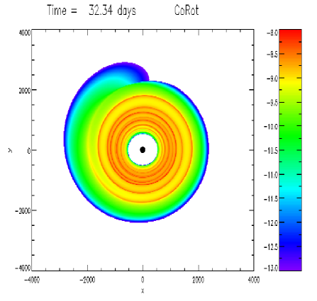
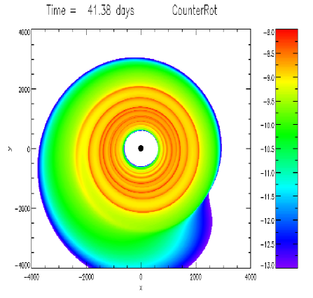
Figure 1: Rest mass density distribution in the co-rotating model CoRot_a.0.9 (left panel) and in the counter-rotating model CounterRot_a.0.9 (right panel) for a recoil velocity $V_{\rm k}=300\,\rm{km}/\rm{s}$ at the time (after merger) when the luminosity reaches a maximum. ${\rm cgs}$ units are reported.

The formulation above is appropriate for numerical integration via standard high-resolution shock-capturing (HRSC) methods developed for the Euler equations (Toro, 1999). All the simulations cover a physical duration much shorter than the viscous time-scale, making the inviscid approximation a very good one. In the following, however, we consider an isothermal evolution of the hydrodynamical equations. Therefore, the temperature of the disc is assumed to be constant in space and in time, and set to the value $T$ reported in Table 1. As a result, there is no need to evolve the energy equation for $U$, since the energy can be computed directly from the temperature and the latter is constant by construction. However, an equation for the time evolution of the internal energy is actually solved

$$\hskip-28.45274pt\partial_{t}(\sqrt{\gamma}W\rho\epsilon)+\partial_{i}[\sqrt{\gamma}\rho\epsilon W(\alpha v^{i}-\beta^{i})]=$$

$$-p\partial_{t}(\sqrt{\gamma}W)-p\partial_{i}(\alpha\sqrt{\gamma}u^{i})\ ,$$ (9)

where $\epsilon$ is the specific internal energy and $p=\rho\epsilon(\gamma-1)$. The solution of Eq. (3) allows to obtain a good estimate of the emitted luminosity, assuming that all the changes in the temperature produced by local compressions will be dissipated away as radiation. This idea, proposed in the Newtonian framework by Corrales et al. (2010), has been first implemented in a general relativistic context by Zanotti et al. (2010). The luminosity is then computed in the following way: the time-update of Eq. (3) provides the value of the quantity $\rho\epsilon$ at time $t^{n+1}=t^{n}+\Delta t$, where $\Delta t$ is the time-step of the simulation. After that, a volume integration of the difference $\rho[\epsilon-\epsilon(T)]$ is performed, where $\epsilon(T)=k_{B}T/[m_{p}(\gamma-1)]$ is the value prescribed by the assumption of isothermal evolution. Finally, division by $\Delta t$ provides the luminosity. The specific internal energy is reset to $\epsilon=\epsilon(T)$ after each time-step, so as to guarantee that the evolution is isothermal. In practice, Eq. (3) is evolved in time with the only aim of computing the difference $\rho[\epsilon-\epsilon(T)]$, which is then assumed to be radiated instantaneously.

The radial numerical grid is discretised by choosing $N_{r}=1200$ points, non-uniformly distributed from $r_{\mathrm{min}}=100M$ to $r_{\mathrm{max}}=6000M$, while outflow boundary conditions are adopted both at $r_{\mathrm{min}}$ and $r_{\mathrm{max}}$. The azimuthal grid extends from $0$ to $2\pi$, with symmetric (i.e. periodic) boundary conditions adopted at $\phi=0$, while the number of angular grid points is $N_{\phi}=200$. All runs are performed with a Courant-Friedrichs-Lewy coefficient ${\rm CFL}=0.5$. We have verified through a series of tests that the choice $(N_{r},N_{\phi})=1200\times 200$ suffices to find a converged solution, and, in consequence, all models have been computed with this canonical resolution.

4 Results

As shown numerically for the first time by Lippai et al. (2008), and then confirmed repeatedly by several authors (O’Neill et al., 2009; Corrales et al., 2010; Rossi et al., 2010; Megevand et al., 2009; Anderson et al., 2010; Zanotti et al., 2010), the combined effects of mass loss from the central black hole and of the recoil velocity generate a spiral shock pattern that transports angular momentum outwards, and become responsible of an enhanced luminosity.

Figure 1 shows the iso-density curves of the rest mass density in the two models CoRot_a.0.9 and CounterRot_a.0.9, plotted when the emitted luminosity reaches its maximum. Because the recoil velocity is not large, neither of the two discs has penetrated into the central cavity at this time. However, the spiral structure is still clearly visible, producing regions of high compression. The role of this spiral pattern has been somewhat overestimated in previous analysis. Indeed, as shown by Zanotti et al. (2010) through the use a sophisticated shock detector, such spiral pattern is not always a true physical shock. In addition, the same pattern can be obtained even in the absence of a mass loss or of a recoil velocity, being produced as the result of non-axisymmetric hydrodynamical instabilities taking place in the disc. Therefore, the spiral pattern cannot be regarded as an unambiguous imprint of a recoiling black hole. It is also worth stressing that, although the inner edge of the accretion disc is placed in a region where general relativistic effects may be regarded as negligible, during the subsequent evolution (later than the time shown in Fig. 1), the central cavity is filled with gas, thus making the relativistic calculation pertinent.

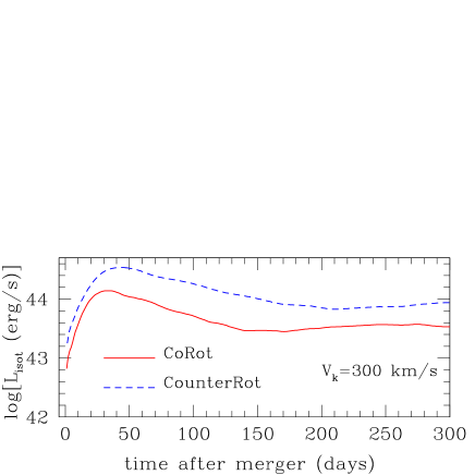
Figure 2: Luminosity computed through the isothermal evolution for the co-rotating model CoRot_a.0.9 and the counter-rotating one CounterRot_a.0.9.

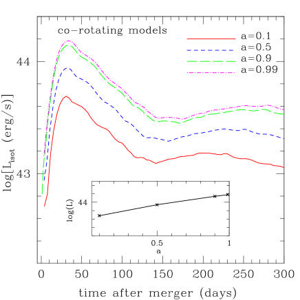
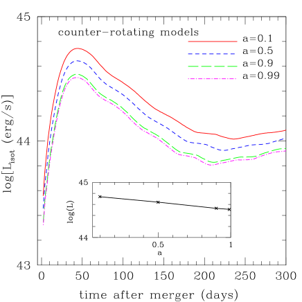
Figure 3: Dependence of the luminosity on the spin of the black hole for corotating (left panel) and for counter-rotating (right panel) models. The insets show the peak luminosity as a function of the black hole spin.

Figure 2, on the other hand, shows the electromagnetic luminosity computed according to the procedure described in Sec. 3. The negative contributions that are produced in regions experiencing rarefactions have been neglected. Because when accounted for these negative contributions typically yield values that are a factor $\sim 2-5$ smaller, the values in Fig. 2-Fig. 4 should be taken as upper limits to the emitted luminosity (see Corrales et al., 2010). More details regarding this approximation can be found in Zanotti et al. (2010), where such an approach is compared to alternative ones for extracting a luminosity in the absence of a fully radiation hydrodynamics treatment. The two curves refer to the models CoRot_a.0.9 and CounterRot_a.0.9, having the same temperature $T=2.68\times 10^{6}{\rm K}$ and the same polytropic constant, subject to a recoil velocity $V_{\rm k}=300\,\rm{km}/\rm{s}$ and with a mass loss after the merging event that amounts to $2\%$ of the initial mass of the black hole. As initially put into evidence by the analysis of  Daigne and Font (2004), counter-rotating models have larger extension with respect to co-rotating ones and, in addition, have a larger radius of the maximum rest mass density point. These two facts are ultimately responsible for the different behavior of the light curves reported in Fig. 2. Because $r_{\rm c}$ is larger for CounterRot_a.0.9 than for CoRot_a.0.9, the spiral shock that forms after the merger event takes longer to reach the region of maximum rest-mass density, which is also the region of highest compressions where most of the luminosity is emitted. As a result, the time of the maximum luminosity is $t_{\rm peak}\sim 32$ days for model CoRot_a.0.9 and $t_{\rm peak}\sim 41$ days for model CounterRot_a.0.9. Moreover, the maximum luminosity at the peak is $L\sim 1.3\times 10^{44}{\rm erg/s}$ for model CoRot_a.0.9 and $L\sim 3.4\times 10^{44}{\rm erg/s}$ for model CounterRot_a.0.9. In a second and tightly related series of simulations the dependence of the light curves on the spin of the central black hole has been investigated, while keeping the same temperature within the discs. When the spin of the black hole is increased, the radius of the maximum rest-mass density $r_{\rm c}$ moves towards the center for co-rotating models, while it moves towards larger distances for counter-rotating models (see Tab. 1). Moreover, when the spin of the black hole is increased, the size of the disc increases for co-rotating models, while it decreases for counter-rotating models. Because of this, changing the spin of the black hole has opposite effects on the emitted luminosity for the two classes of models, as reported in Fig. 3. Indeed, the fluid compression, and therefore the energy released, is larger if it takes place deeper in the potential well, where the effects of the spiral shock are stronger. This explains why increasing the spin of the central black hole produces more luminous co-rotating discs and less luminous counter-rotating ones, as schematically represented by the insets of Fig. 3. Tab. 2 provides an additional information, by showing the ratio of the peak luminosity between counter-rotating and co-rotating discs, in terms of the spin of the black hole. Because of the anti-correlation highlighted above, the discrepancy in the luminosity between the two classes of models is higher at smaller spins.

Table 2: First column: black hole spin. Second column: ratio of the peak luminosity between counter-rotating models and co-rotating models. Third column: difference (in days) between the times of the peak in counter-rotating and in co-rotating discs.

$a$	$\left(L_{\rm Counter}/L_{\rm Corot}\right)_{\rm peak}$	$\left(t_{\rm Counter}-t_{\rm Corot}\right)_{\rm peak}$
		$(d)$
$0.1$	$11.74$	$11.6$
$0.5$	$5.12$	$11.5$
$0.9$	$2.45$	$9.5$
$0.99$	$2.13$	$9.2$

Finally, in a last series of simulations the dependence of the emitted luminosity on the disc temperature has been considered. The results of these analysis have been reported in Fig. 4, which shows the light curves for five models having the same rotation law and the same spin of the central black hole, while different disc temperatures. An almost linear increase of the peak luminosity (see inset of Fig. 4) with the disc temperature has been found, with $L_{\rm peak}\sim 1.3\times 10^{45}{\rm erg/s}$ for $T\sim 1.6\times 10^{7}K$. Such a linear increase is not a surprising result, given the fact that the luminosity is computed from local variations of the specific internal energy and that the latter scales like $\epsilon\propto T$. Finally, the linear increase of the peak luminosity with the disc temperature, which has been reported in Fig. 4 for counter-rotating models, is not affected by the rotation law, and the same linear dependence has been found also for co-rotating models.

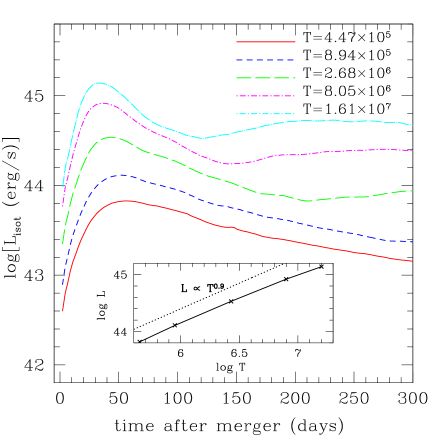
Figure 4: Light curves for different values of the disc temperature in counter-rotating models.

5 Conclusions

We have performed two dimensional (on the orbital plane) relativistic isothermal hydrodynamical simulations of counter-rotating circumbinary discs that react to the mass loss and to the recoil velocity of the central black hole after a merging event of supermassive black holes. These calculations are very relevant for correlating the electromagnetic signal to the gravitational one, in view of the planned Laser Interferometric Space Antenna (LISA) mission. In this respect, after considering the dynamical response of a disc to a typical recoil velocity $V_{\rm k}=300\,\rm{km}/\rm{s}$ oriented on the orbital plane, the results show that the maximum luminosity of counter-rotating discs is a factor $\sim 2$ higher than in co-rotating discs for high spinning black holes, while it is a factor $\sim 12$ higher for slowly rotating black holes. On the other hand, the peak of the luminosity typically happens $\sim 10$ days later with respect to the co-rotating case, with only a weak dependence on the spin of the black hole. All of these effects are due to the different sizes and characteristic radii in the two classes of models. In particular, when the spin of the resultant black hole is larger, co-rotating discs in the post-merger phase are more luminous, while counter-rotating discs are less luminous.

References

- Anderson et al. (2010) M. Anderson, L. Lehner, M. Megevand, D. Neilsen, Phys. Rev. D 81 (2010) 044004.
- Babak et al. (2011) S. Babak, J.R. Gair, A. Petiteau, A. Sesana, Classical and Quantum Gravity 28 (2011) 114001–+.
- Bekenstein (1973) J.D. Bekenstein, Astrophys. J. 183 (1973) 657–664.
- Bode et al. (2010) T. Bode, R. Haas, T. Bogdanovic, P. Laguna, D. Shoemaker, Astrophys. J. 715 (2010) 1117–1131.
- Bogdanović et al. (2011) T. Bogdanović, T. Bode, R. Haas, P. Laguna, D. Shoemaker, Classical and Quantum Gravity 28 (2011) 094020–+.
- Campanelli et al. (2007) M. Campanelli, C.O. Lousto, Y. Zlochower, D. Merritt, Astrophys. J. 659 (2007) L5–L8.
- Chang et al. (2010) P. Chang, L.E. Strubbe, K. Menou, E. Quataert, Mon. Not. R. Astron. Soc. 407 (2010) 2007–2016.
- Coccato et al. (2011) L. Coccato, L. Morelli, E.M. Corsini, L.M. Buson, A. Pizzella, D. Vergani, F. Bertola, ArXiv e-prints (2011).
- Corrales et al. (2010) L.R. Corrales, Z. Haiman, A. MacFadyen, Mon. Not. R. Astron. Soc. 404 (2010) 947–962.
- Daigne and Font (2004) F. Daigne, J.A. Font, Mon. Not. R. Astron. Soc. 349 (2004) 841–868.
- Del Zanna et al. (2007) L. Del Zanna, O. Zanotti, N. Bucciantini, P. Londrillo, Astron. Astrophys. 473 (2007) 11–30.
- Haiman et al. (2009) Z. Haiman, B. Kocsis, K. Menou, Z. Lippai, Z. Frei, Classical and Quantum Gravity 26 (2009) 094032.
- Herrmann et al. (2007) F. Herrmann, I. Hinder, D. Shoemaker, P. Laguna, R.A. Matzner, Astrophys. J. 661 (2007) 430–436.
- Koppitz et al. (2007) M. Koppitz, D. Pollney, C. Reisswig, L. Rezzolla, J. Thornburg, P. Diener, E. Schnetter, Phys. Rev. Lett. 99 (2007) 041102.
- Kozlowski et al. (1978) M. Kozlowski, M. Jaroszynski, M.A. Abramowicz, Astron. and Astrophys. 63 (1978) 209–220.
- Lippai et al. (2008) Z. Lippai, Z. Frei, Z. Haiman, Astrophys. J. 676 (2008) L5–L8.
- Liu and Shapiro (2010) Y.T. Liu, S.L. Shapiro, Phys. Rev. D 82 (2010) 123011.
- MacFadyen and Milosavljević (2008) A.I. MacFadyen, M. Milosavljević, Astrophys. J. 672 (2008) 83–93.
- Megevand et al. (2009) M. Megevand, M. Anderson, J. Frank, E.W. Hirschmann, L. Lehner, S.L. Liebling, P.M. Motl, D. Neilsen, Phys. Rev. D. 80 (2009) 024012.
- Mösta et al. (2010) P. Mösta, C. Palenzuela, L. Rezzolla, L. Lehner, S. Yoshida, D. Pollney, Phys. Rev. D 81 (2010) 064017.
- Nixon et al. (2010) C.J. Nixon, P.J. Cossins, A.R. King, J.E. Pringle, ArXiv e-prints (2010).
- O’Neill et al. (2009) S.M. O’Neill, M.C. Miller, T. Bogdanović, C.S. Reynolds, J.D. Schnittman, Astrophys. J. 700 (2009) 859–871.
- Palenzuela et al. (2010) C. Palenzuela, L. Lehner, S. Yoshida, Phys. Rev. D 81 (2010) 084007.
- Pollney et al. (2007) D. Pollney, et al., Phys. Rev. D 76 (2007) 124002.
- Redmount and Rees (1989) I.H. Redmount, M.J. Rees, Comments on Astrophysics 14 (1989) 165.
- Rezzolla (2009) L. Rezzolla, Class. Quant. Grav. 26 (2009) 094023.
- Robinson et al. (2010) A. Robinson, S. Young, D.J. Axon, P. Kharb, J.E. Smith, Astrophys. J. 717 (2010) L122–L126.
- Rossi et al. (2010) E.M. Rossi, G. Lodato, P.J. Armitage, J.E. Pringle, A.R. King, Mon. Not. R. Astron. Soc. 401 (2010) 2021–2035.
- Rubin et al. (1992) V.C. Rubin, J.A. Graham, J.D.P. Kenney, Astrophysical Journal, Letters 394 (1992) L9–L12.
- Sesana et al. (2009) A. Sesana, M. Volonteri, F. Haardt, Classical and Quantum Gravity 26 (2009) 094033–+.
- Shapiro (2010) S.L. Shapiro, Phys. Rev. D 81 (2010) 024019.
- Stavridis et al. (2009) A. Stavridis, K.G. Arun, C.M. Will, Phys. Rev. D 80 (2009) 067501–+.
- Toro (1999) E.F. Toro, Riemann Solvers and Numerical Methods for Fluid Dynamics, Springer-Verlag, 1999.
- Zanotti et al. (2010) O. Zanotti, L. Rezzolla, L. Del Zanna, C. Palenzuela, Astron. Astrophys. 523 (2010) A8+.