∎
Rovibrational interactions in linear triatomic molecules:
a theoretical study in curvilinear vibrational
coordinates††thanks: Dedicated to Professor Małgorzata Witko on the occasion
of her 60th birthday
Abstract
A variational solution to the rovibrational problem in curvilinear vibrational coordinates has been implemented and used to investigate the nuclear motions in several linear triatomic molecules, like HCN, OCS, and HCP. The dependence of the rovibrational energy levels on the rotational quantum numbers and the -doubling has been studied. Two approximations to the rovibrational Hamiltonian have been examined, depending on the level of truncation of the potential energy operator. It turns out that truncation after the fifth order in the potential is sufficient to produce vibrational energies of high accuracy. An interesting feature of the present formulation of the problem in terms of the curvilinear vibrational coordinates is the explanation for the -doubling of the rovibrational levels, which in this picture is interpreted as the result of the inequivalency of the average rotational constants in mutually perpendicular planes, rather than as the effect of the Coriolis-type interactions between the vibrational and rotational motions. The present theoretical results are compared with the available experimental data from high-resolution spectroscopy, as well as with other ab initio calculations.
Keywords:
rovibrational spectra curvilinear vibrational coordinates anharmonicity -doubling HCN OCS HCP1 Introduction
A proper description of the interactions between the rotational and vibrational motions is an important issue in molecular spectroscopy and the first attempts to find a theoretical solution date back to the beginning of the previous century. Even a short overview of the most important methods is beyond the capacities of a single research paper, so we therefore refer the reader to a recent tutorial overview of the existing approaches tennyson2010 , and restrict ourselves to a necessarily incomplete review of the literature referring to successful implementations of the methods directly related to the topic of our paper.
The choice of the variational method has several advantages over the perturbational theory alternative. Although in many cases perturbation theory allows for a physically sound interpretation of the results, as is the case with the rovibrational energy levels, its possible drawbacks involve among other things the convergence problems of the perturbation series, which do not appear if the variational alternative is used. The variational method is therefore much more robust, especially if many states are to be treated at once and if Fermi resonances are expected. One of the earliest attempts to solve the vibrational problem with the variational method was reported in Ref. carney1975 utilizing the Watson Hamiltonian wf1 . Still other applications of this type can be found, e.g., in Refs. csaszar2007 ; csaszar2009 . A solution to the full rovibrational problem for a linear molecule based on the isomorphic Watson Hamiltonian in the linear normal coordinates with a basis set spanned by the 2 harmonic oscillator eigenfunctions in a polar form is in being sought in our laboratory Shirkov:unp . In Ref. carter1983 a method to solve the variational rovibrational problem for linear triatomic molecules has been reported, which was then developed in Refs. carter1990 ; martinez2006 . However, the methods mentioned above employ internal vibrational coordinates with the exact vibrational Hamiltonian, which make them difficult to extend to systems with more than three atoms. The mixed variational-perturbative approach used by Suzuki sf1 ; sf2 ; sf3 should also be mentioned in this context.
The well-known variational approach to triatomic molecules was implemented by Tennyson et al. hf6 ; hf7 within the dvr3d software package, which allows the solving of the full rovibrational problem. An example application of dvr3d for the HCN and HNC molecules can be found in Ref. tennyson2002 . However, in the method of Tennyson et al. the Jacobi or Radau coordinates are used for the exact (within the Bohr-Oppenheimer approximation) Hamiltonian, which makes it difficult to extend to molecules with a larger number of atoms. It is also worth mentioning the Hougen-Bunker-Johns approach for nonrigid molecules bunker1998 ; konarski1991 implemented in the trove package trove2007 . The illustrative application of this approach can be found in Ref. yurchenko2008 for HDO and Ref. yachmenev2010 for HSOH. However, in the Hougen-Bunker-Johns approach linear molecules should be treated in a special way jensen1983 , and we are not aware of any implementation of this method for this particular (linear) case.
The method presented in this paper is more universal and can be applied to larger molecules, both linear and nonlinear. It was proposed for the first time by Pavlyuchko pavlyuchko1988 and is in principle limited only by the computational costs of the calculation of the potential energy surface (PES) and by the dimensions of the largest block of the resulting rovibrational Hamiltonian matrix. Some attempts to implement this method for linear molecules have been undertaken recently Pavlyuchko:conf , but up to now no results obtained with this approach are available in the literature. It is worth noting that many features of the rovibrational problem depend on the way in which the vibrational and rotational coordinates are introduced. The interpretation of the -doubling is one of the prominent examples bf6 ; Watson:2001 .
The molecules selected for the first test of the new implementation of the rovibrational motion problem are three triatomic molecules: HCN, HCP, and OCS. The first two molecules contain a light hydrogen atom and show a large amplitude vibration, while OCS is a rigid molecule with a low amplitude of the bending mode. Additionally, for the HCN and HCP pair, the effects of introducing a heavier atom belonging to the same group can be examined.
All three selected molecules are of considerable astrophysical and astrochemical interest. Among them HCN is undoubtefully the most widespread one, and numerous experimental and theoretical studies have been undertaken regarding this molecule (see e.g., Refs. maki1974 ; Winnewisser:1976 ; maki1996 ; maki2000 ; mellau2008 ). It is also one of the most prominent interstellar and circumstellar molecule. The degenerate bending mode is an important feature of HCN because of the large amplitude of motion of the light hydrogen atom and also because the bending motion is a direct pathway to the HNC isomer.
Theoretical and experimental data for the OCS molecule can be found in Refs. maki1974 ; naim1998 ; Suvernev:1997 ; Muertz:2000 . Spectroscopic interest in the OCS molecule stems from the fact that this molecule is present in the Venus atmosphere along with the more abundant carbon dioxide Krasnopolsky:2010 . Experimental high-resolution rovibrational spectra have been recorded and assigned e.g., in Refs. Belafhal:1995 ; hornberger1996 ; Rbaihi:1998 ; Strugariu:1998 ; Frech:1998 ; Toth:2010 , in some cases also for less common isotopomers of OCS. One of the first theoretical analyses of the OCS spectra utilized the semiclassical approach based on the integration of selected trajectories aubanel1988 . Martin et al. Martin:1995 used the quartic force field obtained from the coupled cluster calculations including single, double, and noniterative triple excitations, CCSD(T) Raghavachari:89 , with the cc-pVQZ basis set to find the vibrational levels and some rotational constants for the OCS, CS, H2S and CS2 molecules by the second-order perturbation theory. They found for the carbonyl sulfide molecule a generally good agreement with the available experimental data Lahaye:1987 , although some Fermi resonances had to be accounted for in order to get nearer to the experimental energy levels. For instance, the C=O stretching fundamental band () interacts with the combination band. Peterson et al. Peterson:1991 obtained a stretching PES for the carbonyl sulfide molecule with the fourth-order Møller-Plesset perturbation theory (MP4) and the size-consistency corrected configuration interaction method limited to single and double excitations (CISD) and used them to calculate the stretching bands of OCS as well as the rotational and -doubling constants. Both stretching and bending modes have been examined by Pak and Woods Pak:1997 , who used the CCSD(T) method to obtain the PES of OCS and the second-order perturbation theory for the spectroscopic constants. More recently, Xie et al. Xie:2001 devised a PES capable of reproducing high energy vibrations by refining the force field constants of Pak and Woods Pak:1997 through the fitting to experimental vibrational levels up to 8000 cm-1.
The methylidynephosphine molecule HCP is an unstable species which decomposes after several hours in room temperature conditions Gaumont:1994 , but it belongs to a small number of phosporus-containing molecules present in the interstellar media Lattelais:2008 and is therefore of considerable astrochemical interest. From the chemist’s point of view this molecule is a rare example of the existence of the unusual CP triple bond. Interest in the spectroscopic characteristics of HCP grew in the early nineties of the last century due to speculations about the presence of this molecule in some planetary atmospheres Turner:1990 . For its detection in such environments a detailed knowledge of the laboratory rotation-vibration spectrum is required. Experimental examination of the HCP spectra has been reported e.g. in Refs. Tyler:1963 ; lehman1985a ; jung1997 ; Drean:1996 ; Bizzocchi:2001 . The quality of these measurements ranges from the earliest low-resolution spectra to the most recent high-resolution ones. The theoretical work on this molecule usually included the calculation of the PES, which in some cases was then utilized to reproduce vibrational levels and rotational constants lehman1985a ; koput1997 ; Drean:1996 ; Beck:2000 . Koput and Carter koput1997 used the variational method for the vibrational problem followed by the perturbation theory to describe the coupling between rotations and vibrations. Specifically, perturbation theory was applied to calculate the rotational constants with the PES calculated at the CCSD(T) and the second-order Møller-Plesset perturbation theory (MP2) levels of theory. Koput and Carter koput1997 concluded that the MP2 level is not sufficient to reproduce the rovibrational spectra, while the CCSD(T) method is capable of doing so provided that large enough orbital basis is used in the calculations. The basis set effect is particularly important for the vibrational energy levels, while the anharmonic constants are reproduced quite well in the smallest cc-pVTZ basis. Koput and Carter koput1997 also tested the influence of the correlation contributions of the core electrons to the vibrational and rotational parameters. They concluded that the core electrons’ correlation shifts the vibrational levels to higher energies and has little influence on other constants. This line of study has been continued by Beck et al. Beck:2000 who calculated the potential energy surface with the multireference configuration interaction method limited to single and double excitations (MRCI) and used it to calculate high vibrational states and the first rotational constant . Among other theoretical works on HCP one should mention the study of polyads of highly excited vibrational states with the Fermi resonance Hamiltonian Joyex:1998 .
In this paper the implementation of the Rayleigh-Ritz variational solution for the rovibrational problem with the Hamiltonian expressed in the curvilinear vibrational coordinates and the Euler angles is reported and applied to a number of small triatomic molecules. The simplicity of the proposed method follows from the polynomial representation of the potential energy surface and the one-dimentional (1) harmonic oscillator functions in the basis set. In contrast to most of the other approaches employing the curvilinear coordinates, here the variational method is used for the full rovibrational problem, and not just for its vibrational part, which allows for the larger flexibility of the method compared to the perturbation theory. With the present implementation we calculated selected rovibrational levels of HCN, HCP, and OCS up to 13000 cm-1. For higher energies the polynomial representation of the potential energy operator becomes inappropriate and one needs a Morse-like potential and Morse oscillator functions in the basis set. In this case the matrix elements of the Hamiltonian become much more complicated gribov1998 ; requena1986 . However, we believe that the current implementation based on the polynomial expansion is sufficient to obtain and interpret many low-energy rovibrational spectra. In our investigation we paid a special attention to the rovibrational interactions, caused by the dependence of the inverse inertia matrix on the vibrational coordinates. The rovibrational levels were obtained up to and including , then fitted to the known functional form including rotational centrifugal constants and constants of the -resonance and, finally, compared with the available experimental data.
The plan of this paper is as follows. In section 2 we present the mathematical approach to solve the problem of nuclear motion in polyatomic molecules based on the Hamiltonian written in the curvilinear vibrational coordinates and show some advantages of this Hamiltonian over a Hamiltonian expressed in terms of linear vibrational coordinates. In section 3 we report the details of the Rayleigh-Ritz variational procedure, discuss the choice of the basis set functions, and the way the potential energy function should be treated. In section 4 the analytical fitting of the rovibrational energy levels, which are widely used to represent the experimental data, are discussed. The same analytical expressions are utilized to fit the computed energy levels. Section 5 gives an explanation of the -doubling effect when the curvilinear coordinates are used. In section 6 we give some computational details of the potential energy calculations and of the matrix diagonalization in the variational procedure. In section 7 we compare our results with previous theoretical calculations and with the data derived from high-resolution spectroscopic experiments. Finally, section 8 concludes our paper.
2 Molecular Hamiltonian
Several ways of dealing with the molecular Hamiltonian describing rovibrational motions have been described in the literature, depending on whether linear or curvilinear vibrational coordinates are used in the vibrational part. In this section the theory in curvilinear coordinates will be presented. We start the theory section by introducing the curvilinear vibrational coordinates McCoy:1991 ; gribov1998 defined as linear combinations of the natural (internal) vibrational coordinates :
| (1) |
The matrix describes the mathematical form of the -mode vibration papousek1982 ; mills1972 . The matrices and are related to one another by the following expression:
| (2) |
where stands for the unit matrix.
The coordinates are also known as curvilinear vibrational coordinates, since they are related nonlinearly to the Cartesian coordinates of the atoms. For linear molecules the natural vibrational coordinates are of two types, corresponding to the bond stretching and to the linear angle bending modes. The latter mode, which is doubly degenerate, is described by two coordinates in the mutually perpendicular planes mills1972 . The kinetic energy operator for a polyatomic molecule can be written as wilson1955 ; gribov1972 :
| (3) |
The vibrational part of the Hamiltonian can be reduced by performing the differentiation gribov1972 ; gribov1998 :
| (4) |
where denote elements of the kinetic matrix and is a nondifferential kinematic operator gribov1998 , also referred to in the literature to the pseudo-potential halonen1988 . The components of the -tensor are well known and can found in Ref. wilson1955 . Some features of for linear molecules are explained in Refs. ferigle1951 ; gans1970 .
The exact dependence of the -matrix on the vibrational coordinates is rather complicated, therefore some approximations should be employed in Eq. (4) in order to obtain tractable formulas. Different approximate treatments of in the curvilinear coordinates have been proposed in the literature gribov1998 . In this work we chose to expand the elements in the Taylor series:
| (5) |
If additionally the pseudopotential is neglected, the following expression for the vibrational Hamiltonian is obtained:
| (6) |
where the kinematic coefficients and in Eq. (6) are defined by the formulas:,
| (7) |
It should be noted that for linear molecules the matrix of the coefficients is composed of two submatrices, corresponding to stretching and degenerate bending modes with no cross-terms. This explains why the only non-vanishing components of are and , the letters and refering to the bending and stretching coordinates, respectively.
The total Hamiltonian describing the rovibrational motions of a polyatomic molecule can be expressed through the curvilinear vibrational coordinates and the Euler angles which describe the rotation of the axes of the equilibrium inertia tensor with respect to the laboratory frame pavlyuchko1988 :
| (8) |
where denote elements of the inverse inertia tensor matrix. To obtain a working expression for Eq. (8), we expand at the equilibrium point in the curvilinear vibrational coordinates through the second order:
| (9) |
In order to find the derivatives appearing in Eq. (9) the expansion coefficients of the inertia tensor in the linear normal coordinates are used:
| (10) |
Explicit expressions for the coefficients and are well known in the literature tf8 . The coefficients and can then be expressed through the and terms, cf. Ref. gribov1998 for the details.
We also have to note that linear molecules have vibrational degrees of freedom and the inertia tensor has only two main axes, and . The vibrational modes can be classified as doubly-degenerate bending modes and stretching modes. Degenerate modes are described by two coordinates in the perpendicular planes mills1972 . The internal bending coordinate is introduced as , where is the angle of the distortion from linearity. In our ab initio calculations we used instead of , because one can approximately set for small values of .
The rovibrational Hamiltonian expressed through the curvilinear vibrational coordinates, Eq. (4), does not contain Coriolis-type rovibrational interaction terms, i.e. terms of the type and , which are present in the rovibrational Watson Hamiltonian derived in Refs. wf1 ; wf3 . The Hamiltonian given by Eq. (8) contains just the centrifugal interaction terms since depends on the vibrational coordinates only. The other advantage of the latter Hamiltonian form is that there is no need for the special treatment of linear molecules as in the case of the Watson Hamiltonian.
3 The variational solution to the rovibrational problem
In order to find the rovibrational energy levels we have to solve the rovibrational problem described by the Hamiltonian given in Eq. (8), i.e. to solve the following Schrödinger equation:
| (11) |
where denotes a super-index containing quantum numbers corresponding to the vibrational () and the rotational () degrees of freedom, i.e. . To solve the eigenproblem given by Eq. (11) we follow the algorithm described in Ref. pavlyuchko1988 , where the Rayleigh-Ritz variational method is applied. In this algorithm the wave function is expanded in a basis of known functions :
| (12) |
where the basis function is a product of a vibrational function and rotational function :
| (13) |
The functions are solutions to the Schrödinger equation for the symmetric top
| (14) |
where are the Wigner -functions zare1988 . The dimension of the basis set can be minimized if the vibrational functions are variational solutions to the multidimensional vibrational Schrödinger equation:
| (15) |
In Eq. (15) stands for several vibrational indices, e.g. for a linear triatomic molecule . Here are the indices of the basis set functions describing the motion in the perpendicular planes of the degenerate bending mode.
The vibrational problem, Eq. (15), is solved in a basis set constructed from the products of the 1 harmonic oscillator eigenfunctions for each vibrational degree of freedom:
| (16) |
where is the Hermite polynomial of the th order and is the normalization constant. We have also introduced , a dimensionless coordinate, , is the harmonic force constant for the th vibrational mode, and the Planck constant in the appropriate unit system. In the particular case of a linear triatomic molecule the multidimensional vibrational wave function is expanded as:
| (17) |
The last remaining issue for the pure vibrational problem is the representation of the potential energy operator . Usually the Taylor expansion around the equilibrium point truncated after the lowest few terms is used in practical calculations. The Taylor expansions of the potential energy function in both the internal and curvilinear coordinates are listed below:
| (18) |
| (19) |
With the help of Eqs. (18) and (19) the expansion coefficients (for the internal coordinates) and (for the curvilinear vibrational coordinates) are implicitly defined. The coefficients are obtained from the coefficients, which in turn are calculated by an ab initio method. The corresponding transformation formulas for the curvilinear vibrational coordinates are given by the following equations mills1972 :
| (20) |
This transformation is simpler than the analogous expression for the linear vibrational coordinates watson2001 since no higher-order components of the tensor appear in Eq. (20). Of course, in the harmonic approximation both approaches (linear and curvilinear) are fully equivalent.
In a finite basis of the functions , the solution of the rovibrational problem, Eq. (11), is reduced to the diagonalization of the Hermitian matrix with the following matrix elements:
| (21) |
This general formula can greatly be simplified if the structure of the rovibrational Hamiltonian, Eq. (8), the properties of the vibrational basis functions, and the known selection rules for the Wigner -functions are all taken into account. After some algebra pavlyuchko1988 , the following equation for the element of the Hamiltonian matrix is obtained:
| (22) |
where the quantities are defined as:
| (23) |
It should be stressed that are the coefficients that determine the rovibrational interactions. The diagonal terms in Eq. (23) can be interpreted as effective rotational constants for the th vibrational state, while the off-diagonal terms are responsible for the interactions of different vibrational energy levels with rotational motion. All coefficients appearing in the equations above can be found in Ref. pavlyuchko1988 .
For the diagonalization of the Hamiltonian matrix gives pure vibrational energy levels. For states with rovibrational interactions appear. Their physical nature is centrifugal since the elements of the matrix from Eq. (8) depend on the vibrational coordinates . Obviously, neglecting of the dependence of the matrix on the vibrational coordinates by taking only the first term in the expansion given by Eq. (9), makes the matrix , Eq. (23), diagonal. In this case the rovibrational problem can be separated into pure vibrational and pure rotational problems.
4 Constants of rovibrational interactions for linear triatomic molecules
The formulas for the constants of rovibrational interactions and for -doubling are well known in the literature. However, for the sake of completeness and to introduce the notation we repeat them here. The rovibrational levels for the linear top have been derived in Refs. amat1958_1 ; amat1958_2 and are taken in the present form from Refs. maki1996 ; maki2000 ; zelinger2003 ; mellau2008 .
The rotational energies for a given vibration, as obtained from Eq. (11), can be expressed in the following form:
| (24) |
where and denote diagonal and non-diagonal parts of the expression, respectively. The diagonal part is given by the following formula:
| (25) |
where denotes the vibrational quantum numbers, , is the rotational constant, and and are the quadratic and cubic constants of the centrifugal distortion, respectively. The non-diagonal term was fitted to the following expression mellau2008 :
| (26) |
Here, stands for some effective perturbation Hamiltonian used in Ref. mellau2008 . In the particular case of the (01±10) vibrational states we have:
| (27) |
More formulas for the vibrational states (0200), (02±20) and (00) can be derived from Eq. (26). The nonzero constants , , , , and result from the dependence of on , cf. Eq. (9). It should be noted that the variational approach allows the calculating of the dependence of and on , while perturbation theory allows us to find these constants only for the ground vibrational state carney1975 ; koput1997 .
5 Symmetry considerations and -doubling
Triatomic linear molecules have three normal modes: two stretching vibrations usually denoted by and and one degenerate bending vibration denoted by . Depending on the presence or absence of a center of symmetry, linear molecules have either or symmetry. For noncentrosymmetric molecules two stretching vibrations belong to the representation, while the bending has symmetry bunker1998 . The stretching vibrations in this case can usually be approximately attributed to a particular bond, e.g. for the HCN molecule corresponds approximately to the C–H stretch and to the CN stretch.
A few words of explanation are due as far as the nature of the -doubling is concerned. Commonly wf1 ; bf6 , when the rovibrational Watson Hamiltonian for linear molecules is used wf2 , this effect is described by the Coriolis interactions of the rotational and vibrational motions of the molecule. The explanation of the -doubling when the Hamiltonian is expressed in curvilinear vibrational coordinates is different since, as has already been pointed out in Section 2, there is no Coriolis coupling in Eq. (8). In the current approach this effect is explained by the fact that for degenerate molecular deformations in two directions the average values of the inertia tensor are different. As a consequence, for a given vibrational state rotational states with the same absolute value, but with a different orientation of the projection of angular momentum on the symmetry axis , have different values of the rotational constants and therefore also different rotational energy levels. These two possible explanations for the -doubling have been pointed out by Herzberg bf6 .
6 Computational details
Force constants corresponding to the potential energy function , Eq. (18), were calculated at the CCSD(T) level with the molpro suite of programs MOLPRO2010 . The cc-pVQZ basis set was used for all atoms. Only valence electrons were correlated in the CCSD(T) calculations. Since no analytical gradients are available in molpro for the CCSD(T) method, finite-difference formulas were applied in order to obtain the appropriate force constants. This technique naturally limits the maximum order of the force constants that can be calculated with sufficient precision. In order to check the accuracy of the numerical procedure, both 5- and 7-point formulas were used for one-variable derivatives and multi-point formulas for mixed derivatives. Then, only the converged digits were utilized in the subsequent calculations.
The formulas for some exemplary finite-difference fourth derivatives used in this work are given below, where it is assumed that the potential energy function in the internal coordinates is given by . In the derivative calculations the distance increments , and were set equal to 0.01 Å and the angle increment to .
| (28) |
| (29) |
| (30) |
| (31) |
In order to estimate the accuracy of the Taylor expansion for , the series truncated after the fourth and the fifth orders have been used in the production calculations. They are referred to as Approximation 1 and Approximation 2, respectively. Application of Approximation 3, i.e. the series truncated after the sixth order, is unfortunately not possible because of the limited accuracy of the numerical differentiation. Since the calculations reveal that for molecules involving hydrogen atoms the contributions from the fifth order are significant, and hence the sixth-order terms should possibly be included, we expect somewhat larger errors in the rovibrational energy levels for the HCN and HCP molecules.
The rovibrational energies were calculated with a program written by one of our team (L.S.). The masses of the most common isotopes were used in the calculations of the rovibrational spectrum. In all approximations we used the basis set containing 10000 harmonic functions, i.e. 10 basis set functions for each vibrational degree of freedom, which was enough for the convergence of at least the 200 lowest eigenvalues. The Hamiltonian matrix consists of the sub-blocks pertaining to each . However, these subblocks are not independent, since they are connected through the dependence of on the coordinates , and the non-diagonal terms become responsible for the rovibrational interactions. The Davidson algorithm davidson1975 was used to find the lowest eigenvalues and the corresponding eigenvectors of the rovibrational Hamiltonian. The rovibrational energy levels were then assigned by examining the largest weight of the harmonic part for the vibrational levels and the largest weight of the rigid-rotator eigenfunction. In this manual procedure we were able to localize the first 30 vibrational levels. An unambiguous identification for higher energy values turned out to be impossible because of the existence of anharmonic eigenfunctions almost equally distributed between some harmonic eigenfunctions. Special care has to be taken to ensure proper description of the vibration motion within the C–H bond. Because of the presence of the light hydrogen atom this mode is floppy and highly anharmonic. In order to improve this description the “extended” harmonic basis functions have been added to the basis for for the -mode, corresponding to the C–H stretch, utilizing the scaled exponents instead of the harmonic force constants in Eq. (16), where was chosen from the interval (0.5–1.0) to enable better convergence.
7 Results and discussion
In Table 1 equilibrium distances calculated in this work for the molecules under study are presented and compared with the experimental values. An inspection of this Table shows that for all molecules the difference between the experimental and the ab initio distances between the carbon atom with the hydrogen atom is small, about 0.002 Å. Somewhat larger differences, 0.007 and 0.008 Å, are observed for the second distance if the third-row atom is connected to the carbon atom. Most probably, this is a result of neglecting the correlation of the core electrons. However, as pointed out in Ref. Martin:1995 , such a small discrepancy has only a minor effect on the calculated rovibrational constants. Therefore we decided to proceed with the calculations of the CCSD(T) force constants, Eq. (18), with only valence electrons correlated.
For the HCN molecule the importance of various terms in Eqs. (5)–(6) on the computed vibrational energy levels have been examined. The results of these test calculations are listed in Table 2. First, we note that including all the potential energy terms and keeping the simple harmonic oscillator expression for the kinetic energy, cf. the column “Harm.+”, leads to an imbalance in the included contributions which results in an overestimation of the energy levels and in somewhat worse results than the simple harmonic approximation. Adding the anharmonic kinematic coefficients and from Eq. (7) which, together with the potential energy function expanded up to and including the fifth order, lowers the energies making them closer to the experiment. Finally, it is interesting to examine the effect of adding the fifth-order terms in Eq. (5). It turns out that within the latter approximation the errors are reduced only by 1-2 cm-1 for the lowest energy levels. Therefore, we decided to skip in the production calculations. Including of the fifth-order kinematic coefficients might be necessary for higher vibrational energies, especially in view of the fact that the absolute error for the series increases nonlinearly with . However, when dealing with the expansion of the kinetic and potential terms, it is important to take all values of the same order in the Taylor expansion series, because neglecting even some of them may lead to high discrepancies in the final results. This follows from the fact that the variational procedure is very dependent on the non-diagonal terms included in the Hamiltonian matrix. Finally, it is interesting to notice that Approximation 2a gives worse results than Approximation 2 for two high- cases presented in the Table, while for all other cases the latter approach gives slightly worse agreement with the experiment.
For linear molecules the bending coordinates are present only as even powers in the Taylor expansions, so is even with respect to and . This fact is due to the symmetry of the degenerate bending mode with respect to the plane perpendicular to the plane of vibration. We can also note an interesting property of high order force constants containing the bending coordinates, coming from the equivalence of the two bending vibration planes:
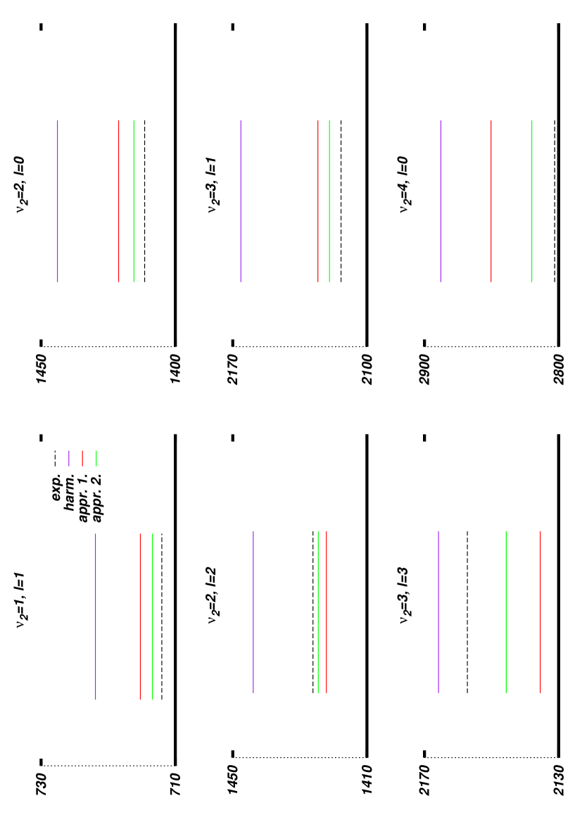
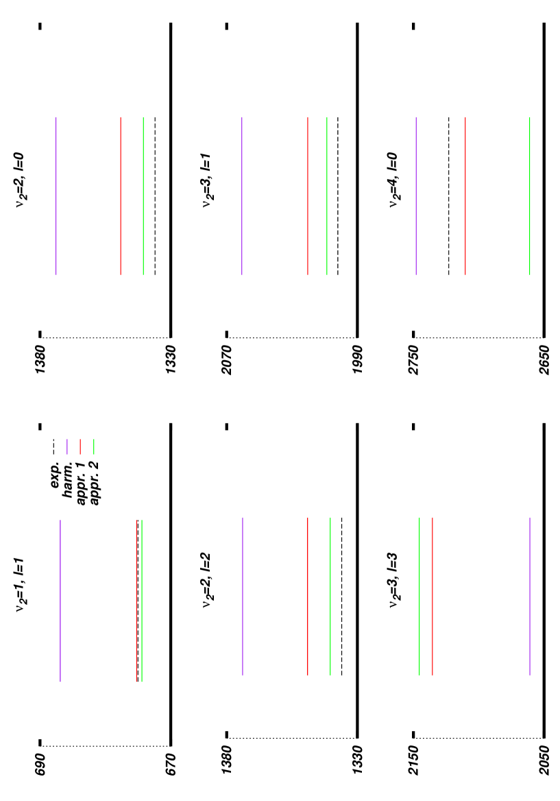
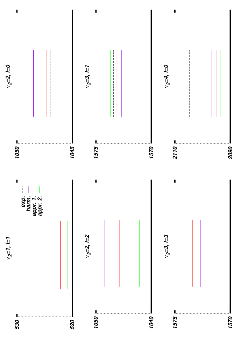
The pure vibrational energy levels relative to the ground-state energy level are listed in Tables 3–5 for the molecules HCN, OCS, and HCP, respectively. In these tables the fundamental energy levels as well as some overtones are presented. Three approximations have been used in these tables: harmonic (Approximation 0), and Approximations 1 and 2 differing in the way in which the operator was truncated, cf. Section 6. The results are compared with the experimental data when available. The experimental data for the energies and rotational constants were taken from Ref. mellau2008 for HCN, Refs. fayt1972 ; schneider1989 ; hornberger1996 for OCS, and Refs. lehman1985a ; jung1997 for HCP. Additionally, Figures 1–3 show selected energy levels for lowest few bending modes of HCN, HCP, and OCS calculated via all three methods and compared with the experiment. Differences between the theoretical and the experimental results are also reported for better readability of the tables.
The results reported in Tables 3–5 show that in the series of approximations, starting with the harmonic and ending with Approximation 2, an increasing accuracy is observed in nearly all cases. Obviously, the harmonic approximation gives the largest errors with respect to the experimental values, and Approximation 1 always improves the agreement with the experiment. The level of improvement varies substantially depending on the molecule and the vibrational mode studied, but often the use of Approximation 1 causes even a five-fold lowering of the energy gap between the calculated and experimental energy levels. Approximation 2 leads in almost all cases to results even closer to the experiment than Approximation 1. It is also interesting to note that our calculations support the claim concerning the high anharmonicity of the C–H stretching mode. For the HCN and HCP molecules these modes are easily identified by looking at the column. They are the only states with errors larger than 100 cm-1. Although both Approximations 1 and especially 2 do a good job of bringing this mode close to the experiment, it could be envisaged that the next approximation would give an even better agreement. Unfortunately, the analytical gradients within the CCSD(T) approach should be used for this purpose. Another way to improve the potential energy surface is to use Morse-like potential for this mode, which corresponds approximately to the C–H stretch. Such potential better describes upper vibrational states close to the dissociation limit, see for example Ref. bowman1993 . Unfortunately, this leads to serious complications in the calculations of the matrix elements and has not been attempted in this paper.
In Tables 3–5 a comparison of our results with previous calculations for every molecule is also presented. As already mentioned above, HCN is the most studied molecule and a vast theoretical material is available in the literature dealing with the problem of the vibrational HCN spectra. In Table 3 we listed values from four different sources. The first column with the theoretical results corresponds to the earliest work utilizing an ab initio PES bowman1993 , where one of the modifications of the DVR method was used to calculate the vibrational energies. The next set of results stems from a more recent implementation of the DVR method tennyson2001 . It should be stressed again that although the DVR method allows finding of vibrational energies up to very high excitation levels, it is limited to triatomic molecules and is therefore less general than the method presented in this paper in the curvilinear coordinates. Another work applying the DVR approach is Ref. csaszar2007 , where DVR was implemented for the Watson Hamiltonian wf1 ; wf2 ; wf3 . The last set of data was produced by Wang et al. wang2000 by applying a finite element method for the Watson Hamiltonian with . A perusal of this part of Table 3 allows us to conclude that the present vibrational energies are generally better than those of Ref. bowman1993 and of the same level of accuracy than in the other references, except DVR implementation made in tennyson2001 where the accuracy is better, especially for combination bands, like (2 00 3) in Table 3. This fact is reassuring in view of the just mentioned possible high-precision of the DVR method for the triatomic molecules.
For carbonyl sulfide much fewer theoretical investigations are available. Since the OCS molecule is rigid, the model with the neglected bending mode can be used to study vibrationally excited stretching states. Such an approach has been pursued by Peterson et al. Peterson:1991 , The vibrational energies obtained in Ref. Peterson:1991 are listed in Table 4. It is not surprising that the discrepancy between these results with the experimental values is larger than in the case of our approach, where the mixed bending-stretching terms have been taken into account. To our knowledge it was the only ab initio available potential energy surface for excited vibrational states. The next column of Table 4 contains the data of Ref. sarkar2009 , where an algebraic model was used to analyze and interpret the experimental rovibrational spectra of small and medium-sized molecules. This method employs the Lie algebra techniques to obtain an effective Hamiltonian operator which describes rovibrational degrees of freedom. Since it does not use any ab initio results, but instead is solely based on the fitting of the spectroscopic data, the results obtained there are very close to the experimental values. Finally, the last theoretical column in Table 4 contains data from Ref. aubanel1988 , where a semi-classical model based on the adiabatic switching method (ASM) was used together with a spectroscopic potential energy function. Also, in this case the good agreement with the experiment can be attributed to the use of some spectroscopic data in the actual calculations. Taking this into account we can conclude that our method reproduces the vibrational energies for OCS much better that the other ab initio approach Peterson:1991 .
The DVR method was also applied to the phosphaethyne molecule beck2000 . The solution to the vibrational problem with an ab initio PES gave ,in general, a slightly better agreement with the experiment than our results. The following column in Table 4 shows the results of Ref. koput1997 , where an ab initio PES was used to computed the rovibrational energy levels with a mixed variational-pertubation theory approach. Also here a somewhat better agreement between the vibrational energy levels and the experiment is found. However, the constants of the rovibrational interactions were calculated only for the ground state in this paper.
Several possible reasons of the remaining discrepancies should be considered. The first issue is the quality of the CCSD(T)/cc-pVQZ electronic energies. Since the CCSD(T) method is known to be very accurate for molecules (unless very large distortions to the geometry are studied) and the cc-pVQZ orbital basis is also quite accurate, we can exclude the possibility that inaccurate electronic energies are the reason for the remaining errors. The most probable cause of the discrepancies are the truncation of the Taylor expansions which we have used for the -tensor and for the potential in the Hamiltonian. For instance, we used the second-order (i.e. linear and quadratic) expansion in the vibrational coordinates of , which may be insufficient for some excited rovibration bending energy levels, if the average geometry of the molecule differs considerably from the equilibrium geometry.
For the CN, CP, and C=S stretching modes, generally larger errors are observed for the fundamental transition than for the other two. Errors of about 5 cm-1 can be seen in the former case and only 1-2 cm-1 for the latter. The error increases approximately twofold for the first overtone (). According to Koput et al. koput1997 this discrepancy can be explained by the effect of neglecting the correlation between the core electrons of the heavier atoms. This hypothesis is supported by the fact that only the mode is so atrongly affected. It seems that further studies of the molecules containing atoms from the third row of the periodic table should account for the core correlation. Similar discrepancies have been found by Martin et al. Martin:1995 .
Finally, one more complication arises from the fact that the values of the matrix elements are very sensitive to small non-diagonal anharmonic elements of the potential function . These elements have a small influence on the calculated rovibrational energy levels, but cause a considerable change in the wave functions, and, hence in the average geometry of the molecule and its rotational energy levels if the molecule is vibrationally excited.
In Tables 6–8 the constants for the rovibrational energies calculated within Approximation 2 are presented. The experimental values for these molecules are also given, when available. These constants have been obtained by first computing rovibrational energy levels for various values of and , and then by performing fitting of the values to the analytic form, cf. Eqs. (24)–(27). The values up to and including =15 were used. The results show that the most important constants, i.e. , , and , are reproduced quite accurately. For the higher-order constants, the accuracy of the calculated rovibrational energies and the truncation of the maximum was found to be insufficient, so the and constants are not reported in Tables 6–8. Apart from the comparison to the experiment it is interesting to examine the dependence of the rotational constants on the vibrational quantum numbers. Such a dependence is especially visible for molecules containing a hydrogen atom, like HCN and HCP. The results allow us to conclude that the constants and grow linearly with , the quantum number for the degenerate bending mode, while for fixed they decrease with , the vibrational angular momentum quantum number for the bending mode . This finding can be explained by the fact that for a molecule in an excited bending mode, the component of becomes smaller which leads to a lowering of the constants and . On the other hand, decreasing the constants while increasing is mostly caused by the interaction of the total angular momentum with the vibrational one. These constants also become smaller when the quantum numbers and increase. This result can be rationalized by the fact as the vibrationally averaged interatomic distance becomes larger, the distance differs more from the equilibrium distance. This assumption can be supported by calculating the vibrationally averaged values of the bond distances fo the molecules under study. Luckily, such calculations were reported by Laurie et al. laurie1962 who presented , Å for the ground state. These values are larger than the equilibrium values from Table 1.
8 Summary
The rovibrational Hamiltonian in curvilinear vibrational coordinates has been used to solve the nuclear motion problem for several linear triatomic molecules in curvilinear vibrational coordinates. The curvilinear coordinates were shown to have advantages over the more commonly used linear coordinates. Comparison with the exising theoretical results shows that the present approach works equally well comparing to other ab initio calculations of vibrational energy levels, and is not limited to triatomic molecules. In its current form the approach presented in this paper provides a good accuracy for most vibrational levels and recovers the rotational and the -doubling constants for the studied molecules. Further improvements to the code will also include the calculation of intensities, so that the full spectrum of the molecules can be simulated.
Acknowledgments
This work was supported by the Polish Ministry of Science and Education through project N N204 215539.
| Molecule | Reference | ||
| HCN | 1.06686 | 1.15646 | this work |
| 1.065 | 1.153 | Winnewisser:1976 | |
| HCP | 1.07216 | 1.54732 | this work |
| 1.070 | 1.540 | Drean:1996 | |
| OCS | 1.15830 | 1.56902 | this work |
| 1.156 | 1.561 | Lahaye:1987 |
| Harm. | Harm. + | Appr. 2 | Appr. 2a | Exp. | |
| 0 11 0 | 721.9 | 727.6 | 713.4 | 712.9 | 712.0 |
| 0 20 0 | 1443.9 | 1447.9 | 1415.4 | 1413.7 | 1411.4 |
| 0 22 0 | 1443.9 | 1460.4 | 1424.5 | 1423.3 | 1426.1 |
| 0 31 0 | 2165.8 | 2170.4 | 2119.6 | 2117.7 | 2113.5 |
| 0 33 0 | 2165.8 | 2190.8 | 2145.6 | 2143.3 | 2157.2 |
| 0 40 0 | 2887.8 | 2926.5 | 2820.1 | 2816.1 | 2803.0 |
| 0 00 1 | 2123.0 | 2148.5 | 2098.1 | 2098.0 | 2096.4 |
| 1 00 0 | 3435.3 | 3554.5 | 3316.8 | 3314.6 | 3311.4 |
| 0 00 2 | 4246.0 | 4231.5 | 4168.2 | 4165.3 | 4173.2 |
| 2 00 0 | 6870.7 | 6934.7 | 6529.4 | 6524.9 | 6519.5 |
| 0 11 1 | 2844.9 | 2898.3 | 2810.5 | 2807.4 | 2805.6 |
| 2 00 3 | 13239.6 | 13432.9 | 12675.1 | 12669.2 | 12658.0 |
| Harm. | Appr. 1 | Appr. 2 | Exp | Ref. bowman1993 | Ref. tennyson2001 | Ref. csaszar2007 | Ref. wang2000 | ||||
| 0 11 0 | 721.9 | 9.9 | 715.2 | 3.2 | 713.4 | 1.4 | 712.0 | 718.4 | 712.0 | 715.9 | 713.0 |
| 0 20 0 | 1443.9 | 32.5 | 1421.1 | 9.7 | 1415.4 | 4.0 | 1411.4 | 1418.9 | 1411.4 | 1414.9 | 1421.6 |
| 0 22 0 | 1443.9 | 17.8 | 1422.1 | -4 | 1424.5 | -1.6 | 1426.1 | n/a | n/a | n/a | n/a |
| 0 31 0 | 2165.8 | 52.3 | 2125.6 | 12.1 | 2119.6 | 6.1 | 2113.5 | 2126.0 | 2113.45 | n/a | 2127.9 |
| 0 33 0 | 2165.8 | 21.8 | 2135.5 | -8.5 | 2145.6 | 1.6 | 2157.2 | n/a | n/a | n/a | n/a |
| 0 40 0 | 2887.8 | 85.8 | 2850.4 | 37.4 | 2820.1 | 18.1 | 2803.0 | 2812.5 | 2807.1 | 2801.5 | 2834.3 |
| 0 00 1 | 2123.0 | 26.6 | 2095.1 | -1.3 | 2098.1 | 1.7 | 2096.4 | 2090.3 | 2091.0 | 2100.6 | 2083.2 |
| 1 00 0 | 3435.3 | 123.9 | 3313.4 | 2 | 3316.8 | 5.4 | 3311.4 | 3334.1 | 3311.5 | 3307.7 | 3340.4 |
| 0 00 2 | 4246.0 | 72.8 | 4181.7 | 8.5 | 4168.2 | -5 | 4173.2 | 4161.5 | 4173.1 | 4181.5 | 4146.3 |
| 2 00 0 | 6870.7 | 351.2 | 6598.4 | 78.9 | 6529.4 | -9.9 | 6519.5 | 6553.2 | 6519.6 | 6513.5 | n/a |
| 0 11 1 | 2844.9 | 39.3 | 2809.4 | 3.8 | 2810.5 | 4.9 | 2805.6 | 2806.4 | 2807.1 | n/a | n/a |
| 2 00 3 | 13239.6 | 581.6 | 12795.1 | 137.1 | 12675.1 | 17.1 | 12658.0 | n/a | 12658.0 | n/a | n/a |
| 0 20 1 | 3566.9 | 64.8 | 3532.1 | 30.0 | 3512.0 | 9.9 | 3502.1 | 3507.4 | 3511.0 | 3511.0 | 3511.0 |
| 0 22 1 | 3566.9 | 44.2 | 3541.7 | 19.0 | 3529.4 | 6.7 | 3522.7 | n/a | n/a | n/a | n/a |
| 1 31 0 | 5601.1 | 232.8 | 5435.7 | 67.4 | 5398.4 | 30.1 | 5368.3 | 5387.1 | n/a | n/a | n/a |
| Harm. | Appr. 1 | Appr. 2 | Exp | Ref. Peterson:1991 | Ref. sarkar2009 | Ref. aubanel1988 | ||||
| 0 11 0 | 524.2 | 3.8 | 522.1 | 1.7 | 520.9 | 0.5 | 520.4 | n/a | n/a | 520.3 |
| 0 20 0 | 1048.4 | 1.4 | 1047.3 | 0.3 | 1047.1 | 0.1 | 1047.0 | n/a | 1047.0 | 1046.9 |
| 0 22 0 | 1048.4 | 1045.7 | 1042.1 | n/a | n/a | n/a | 1048.8 | |||
| 0 31 0 | 1572.7 | -0.7 | 1573.1 | -0.3 | 1573.7 | 0.3 | 1573.2 | n/a | 1569.0 | 1573.4 |
| 0 33 0 | 1572.7 | 1573.4 | 1574.0 | n/a | n/a | n/a | 1561.5 | |||
| 0 40 0 | 2096.9 | -7.9 | 2101.3 | -3.5 | 2102.4 | -2.4 | 2104.8 | n/a | 2088.0 | 2105.8 |
| 0 00 1 | 871.7 | 12.4 | 861.4 | 2.1 | 859.1 | -0.2 | 859.3 | 869.0 | 855.5 | 859.2 |
| 1 00 0 | 2094.7 | 32.4 | 2078.4 | 16.2 | 2067.1 | 4.9 | 2062.2 | 2071 | 2057.9 | 2062.1 |
| 0 00 2 | 1743.4 | 32.7 | 1715.7 | 5 | 1712.7 | 2 | 1710.7 | 1730.0 | 1705.0 | 1710.6 |
| 2 00 0 | 4189.3 | 86.9 | 4127.2 | 25.8 | 4110.7 | 9.3 | 4101.4 | 4119.0 | 4097.1 | 4101.4 |
| 0 11 1 | 1395.9 | 1379.4 | 1373.1 | n/a | n/a | n/a | n/a | 1372.8 | ||
| 2 00 3 | 6804.2 | 6704.1 | 6687.5 | n/a | n/a | n/a | n/a | |||
| 0 20 1 | 1920.1 | 27.9 | 1915.2 | 23.0 | 1899.7 | 7.5 | 1892.2 | n/a | 1895.5 | 1891.7 |
| 0 22 1 | 1920.1 | 1911.4 | 1890.5 | n/a | n/a | 1886.7 | 1890.5 | |||
| 1 31 0 | 3667.4 | 52.0 | 3643.2 | 27.8 | 3618.8 | 3.4 | 3615.4 | n/a | 3617.9 | 3614.4 |
| Harm. | Appr. 1 | Appr. 2 | Exp | Ref. beck2000 | Ref. koput1997 | Ref. sarkar2009 | ||||
| 0 11 0 a | 686.9 | 11.95 | 675.2 | 0.2 | 674.4 | -0.6 | 675 | 675 | 675.2 | n/a |
| 0 20 0 a | 1373.9 | 37.9 | 1349.1 | 13.1 | 1340.4 | 4.4 | 1336 | 1336 | 1335.0 | 1332.9 |
| 0 22 0 a | 1373.9 | 9.9 | 1369.1 | 5.1 | 1365.7 | 1.7 | 1364 | 1364 | n/a | 1340.2 |
| 0 31 0 a | 2060.8 | 58.8 | 2020.4 | 18.4 | 2008.7 | 6.7 | 2002 | 2002 | 2002.1 | 1995.6 |
| 0 33 0 a | 2060.8 | 2041.1 | 2036.1 | n/a | n/a | n/a | n/a | |||
| 0 40 0 b | 2747.8 | 105.0 | 2721.1 | 78.3 | 2715.8 | 73.0 | 2643 | n/a | 2653.8 | n/a |
| 0 00 1 a | 1294.9 | 15.9 | 1287.2 | 8.2 | 1285.1 | 6.1 | 1279 | n/a | 1275.5 | 1279.0 |
| 1 00 0 b | 3345.3 | 129.3 | 3301.7 | 85.7 | 3207.1 | -8.9 | 3217 | n/a | 3215.3 | n/a |
| 0 00 2 a | 2589.8 | 40.8 | 2571.4 | 22.4 | 2570.1 | 21.1 | 2549 | n/a | 2540.1 | 2547.4 |
| 2 00 0 a | 6690.5 | 6671.4 | 6667.8 | n/a | n/a | 6321.0 | n/a | |||
| 0 11 1 a | 1981.8 | 34.8 | 1960.1 | 13.1 | 1955.1 | 8.1 | 1947 | n/a | n/a | n/a |
| 2 00 3 a | 10575.2 | 10384.7 | 10276.7 | n/a | n/a | n/a | n/a | |||
| 0 20 1 a | 2668.8 | 70.8 | 2634.2 | 36.2 | 2608.4 | 10.4 | 2598 | 2598 | n/a | 2597.2 |
| 0 22 1 a | 2668.8 | 42.8 | 2647.2 | 21.2 | 2636.3 | 10.3 | 2626 | 2626 | n/a | 2604.5 |
| 1 31 0 a | 5406.1 | 5302.7 | 5249.7 | n/a | n/a | n/a | n/a |
| Exp | Calc | Exp | Calc | Exp | Calc | |
| 0 00 0 | 1.478222 | 1.479782 | 2.91028 | 2.59259 | ||
| 0 11 0 | 1.481773 | 1.481931 | 2.97746 | 3.01327 | 7.48773 | 7.51431 |
| 0 20 0 | 1.485828 | 1.487207 | 3.04799 | 3.08957 | 7.59561 | 7.63292 |
| 0 22 0 | 1.484997 | 1.483982 | 3.04079 | 3.11047 | ||
| 0 31 0 | 1.489575 | 1.492028 | 3.11365 | 3.19783 | 7.70926 | 7.81492 |
| 0 33 0 | 1.487868 | 1.491873 | 3.10024 | 3.29147 | ||
| 0 11 1 | 1.471574 | 1.475982 | 2.98254 | 3.11873 | 7.47954 | 7.49425 |
| 0 20 1 | 1.475493 | 1.482542 | 3.05017 | 3.78874 | 7.57341 | 7.61422 |
| 0 22 1 | 1.474678 | 1.491012 | 3.04520 | 3.85578 | ||
| 1 31 0 | 1.479809 | 1.481287 | 3.11952 | 4.50034 | 7.85215 | 7.83421 |
| Exp | Calc | Exp | Calc | Exp | Calc | |
| 0 00 0 a | 0.202856 | 0.202506 | 4.341064 | 4.703412 | ||
| 0 11 0 a | 0.203209 | 0.203347 | 4.411467 | 5.198434 | 2.12193 | 2.11932 |
| 0 20 0 b | 0.203480 | 0.203135 | 3.66256 | 3.963137 | n/a | 2.13421 |
| 0 22 0 b | 0.203559 | 0.203397 | 5.23854 | 4.598443 | ||
| 0 31 0 | n/a | 0.203492 | n/a | 4.993237 | n/a | 2.16402 |
| 0 33 0 | n/a | 0.204431 | n/a | 5.194394 | ||
| 0 11 1 a | 0.202657 | 0.203054 | 4.54206 | 5.94217 | 2.28496 | 2.25421 |
| 0 20 1 a | 0.202953 | 0.203384 | 4.55522 | 5.53215 | 2.2238 | 2.18401 |
| 0 22 1 a | 0.203048 | 0.203043 | 4.63515 | 5.73263 | ||
| 1 31 0 | n/a | 0.203349 | n/a | 6.143694 | n/a | 2.17754 |
| Exp | Calc | Exp | Calc | Exp | Calc | |
| 0 00 0 | 0.666326 | 0.667483 | 0.70392 | 0.93820 | ||
| 0 11 0 | 0.666771 | 0.667333 | 0.71196 | 0.99482 | 1.63032 | 1.65339 |
| 0 20 0 | 0.667344 | 0.668391 | 0.719160 | 1.03945 | 1.65970 | 1.68432 |
| 0 22 0 | n/a | 0.663641 | n/a | 1.09384 | ||
| 0 31 0 | 0.667784 | 0.668380 | 0.72502 | 1.10939 | 1.70887 | 1.73283 |
| 0 33 0 | n/a | 0.673452 | n/a | 1.03988 | ||
| 0 11 1 | 0.662932 | 0.665482 | 0.72052 | 0.928438 | 1.56214 | 1.49844 |
| 0 20 1 | n/a | 0.668391 | n/a | 0.91938 | n/a | 1.61925 |
| 0 22 1 | n/a | 0.663942 | n/a | 1.39492 | ||
| 1 31 0 | n/a | 0.653393 | n/a | 1.03821 | n/a | 1.66754 |
References
- (1) Lodi, L., Tennyson, J.: J. Phys. B: At. Mol. Opt. Phys. 43, 133,001 (2010)
- (2) Carney, G.D., Kern, C.W.: Int. J. Quantum Chem. Symp. 9, 317–323 (1975)
- (3) Watson, J.K.G.: Mol. Phys. 15, 479–490 (1968)
- (4) Matyus, E., Czako, G., Sutcliffe, B.T., Csaszar, A.G.: J. Chem. Phys. 127, 084,102 (2007)
- (5) Matyus, E., Simunek, J., Csaszar, A.G.: J. Chem. Phys. 131, 074,106 (2009)
- (6) Shirkov, L., Moszynski, R.: (2011). Work in progress
- (7) Carter, S., Handy, N.C., Sutcliffe, B.T.: Mol. Phys. 49, 745–748 (1983)
- (8) Carter, S., Handy, N.C., Mills, I.M.: Phil. Trans. R. Soc. Lond. A 332, 309–327 (1990)
- (9) Martinez, R.Z., Lehmann, K.K., Carter, S.: J. Chem. Phys. 125, 174,306 (2006)
- (10) Suzuki, I.: Bull. Chem. Soc. Japan 44, 3277–3287 (1971)
- (11) Suzuki, I.: Bull. Chem. Soc. Japan 48, 3565–3572 (1975)
- (12) Suzuki, I.: Bull. Chem. Soc. Japan 52, 1606–1613 (1975)
- (13) Tennyson, J., Henderson, J.R., Fulton, N.G.: Comp. Phys. Comm 86, 175–198 (1995)
- (14) Tennyson, J., Henderson, J.R., Fulton, N.G.: Comp. Phys. Comm 163, 85–116 (2004)
- (15) Harris, G.J., Polyanski, O.L., Tennyson, J.: Spectrochimica Acta Part A 58, 673–690 (2002)
- (16) Bunker, P.R., Jensen, P.: Molecular Symmetry and Spectroscopy. NRC Research Press, Ottawa (1998)
- (17) Konarski, J.: Theoretical Foundations of Molecular Spectroscopy. PWN, Warsaw (1991). (in Polish)
- (18) Yurchenko, S.N., Thiel, W., Jensen, P.: J. Mol. Spectr. 245, 126–140 (2007)
- (19) Yurchenko, S.N., Voronin, B.A., Tolchenov, R.N., Doss, N., Naumenko, O.V., Thiel, W., Tennyson, J.: J. Chem. Phys. 128 (2008)
- (20) Yachmenev, A., Yurchenko, S.N., Jensen, P., Baum, O., Giesend, T.F., Thiel, W.: Phys. Chem. Chem. Phys. 12, 8387–8397 (2010)
- (21) Jensen, P.: Comp. Phys. Rep. 1, 1–55 (1983)
- (22) Pavlyuchko, A.I.: J. Appl. Spectr. 48, 83–88 (1988)
- (23) Pavlyuchko, A.I.: (2009). Reported during the ConfMolMod-6 conference (Russia)
- (24) Herzberg, G.: Molecular Spectra and Molecular Structure, vol. II. Wiley-Interscience, New York (1950)
- (25) Watson, J.K.G.: Can. J. Phys. 79, 521–532 (2001)
- (26) Maki, A.G., Quapp, W., Klee, S., Mellau, G.C., Albert, S.: J. Phys. Chem. Ref. Data 3 (1974)
- (27) Winnewisser, G., Maki, A.G., Johnson, D.R.: J. Mol. Spectr. 261, 395 (1976)
- (28) Maki, A.G., Quapp, W., Klee, S., Mellau, G.C., Albert, S.: J. Mol. Spectr. 180, 323–336 (1996)
- (29) Maki, A.G., Mellau, G.C., Klee, S., Winnewisser, M., Quapp, W.: J. Mol. Spectr. 202, 67–82 (2000)
- (30) Mellau, G.C., Winnewisser, B.P., Winnewisser, M.: J. Mol. Spectr. 249, 23–42 (2008)
- (31) Naïm, S., Fayt, A., Bredohl, H., Blavier, J.F., Dubois, I.: J. Mol. Spectr. 192, 91–101 (1998)
- (32) Suvernev, A.A., Goodson, D.Z.: J. Chem. Phys. 107, 4099–4111 (1997)
- (33) Mürtz, M., Palm, P., Urban, W., Maki, A.G.: J. Mol. Spectr. 204, 281–285 (2000)
- (34) Krasnopolsky, V.A.: Icarus 209, 314–322 (2010)
- (35) Belafhal, A., Fayt, A., Guelachvili, G.: J. Mol. Spectr. 174, 1–19 (1995)
- (36) Hornberger, C., Boor, B., Stuber, R., Demtroder, W., Naim, S., , Fayt, A.: J. Mol. Spectr. 179, 349–353 (1996)
- (37) Rbaihi, E., Belafhal, A., Auwera, J.V., Naïm, S., Fayt, A.: J. Mol. Spectr. 191, 32–44 (1998)
- (38) Strugariu, T., Naïm, S., Fayt, A., Bredohl, H., Blavier, J.F., Dubois, I.: J. Mol. Spectr. 189, 206–219 (1998)
- (39) Frech, B., Mürtz, M., Palm, P., Lotze, R., Urban, W., Maki, A.G.: J. Mol. Spectr. 190, 91–100 (1998)
- (40) Toth, R.A., Sung, K., Brown, L.R., Crawford, T.J.: J. Qualit. Spectr. Rad. Transfer 111, 1193–1200 (2010)
- (41) Aubanel, E.E., Wardlaw, D.M.: J. Chem. Phys. 88, 495–517 (1988)
- (42) Martin, J.M.L., Francois, J.P., Gijbels, R.: J. Mol. Spectr. 169, 445–457 (1995)
- (43) Raghavachari, K., Trucks, G.W., Pople, J.A., Head-Gordon, M.: Chem. Phys. Lett. 157, 479 (1989)
- (44) Lahaye, J.G., Vandenhaute, R., Fayt, A.: J. Mol. Spectr. 123, 48 (1987)
- (45) Peterson, K.A., Mayrhofer, R.C., Woods, R.C.: J. Chem. Phys. 94, 431–441 (1991)
- (46) Pak, Y., Woods, R.C.: J. Chem. Phys. 107, 5094–5102 (1997)
- (47) Xie, D., Lu, Y., Xu, D., Yan, G.: Chem. Phys. 270, 415–428 (2001)
- (48) Gaumont, A.C., Denis, J.M.: Chem. Rev. 94, 1413–1439 (1994)
- (49) Lattelais, M., Pauzat, F., Pilme, J., Ellinger, Y.: Phys. Chem. Chem. Phys. 10, 2089–2097 (2008)
- (50) Turner, B.E., Tsui, T., Bally, J., Guèlin, M., Cernicharo, J.: Astrophys. J. 365, 569–585 (1990)
- (51) Tyler, J.K.: J. Chem. Phys. 40, 1170 (1963)
- (52) Lehmanns, K.K., Harrison, G.R., Ross, S.C., Lohr, L.L.: J. Chem. Phys. 82, 537–566 (1985)
- (53) Jung, M., Winnewisser, B.P., Winnewisser, M.: J. Mol. Struc. 413-414, 31–48 (1997)
- (54) Drean, P., Demaison, J., Poteau, L., Denis, J.M.: J. Mol. Spectr. 176, 139–145 (1996)
- (55) Bizzocchi, L., Thorwirth, S., Müller, H.S.P., Lewen, F., Winnewisser, G.: J. Mol. Spectr. 105, 110–116 (2001)
- (56) Koput, J., Carter, S.: Spectr. Acta A 53, 1091–1100 (1997)
- (57) Beck, C., Schinke, R., Koput, J.: J. Chem. Phys. 112, 8446 (2000)
- (58) Joyex, M., Grebenshchikov, S.Y., Schinke, R.: J. Chem. Phys. 109, 8342 (1998)
- (59) Gribov, L., Pavlyuchko, A.I.: Variational Methods for the Solution of Anharmonic Problems in the Theory of Vibrational Spectra of Molecules. Nauka, Moscow (1998). (in Russian)
- (60) Requena, A., Pineiro, A.L., Moreno, B.: Phys. Rev. A 34, 4480–4386 (1986)
- (61) McCoy, A.B., Sibert III, E.L.: J. Chem. Phys. 95, 3476–3487 (1991)
- (62) Papousek, D., Aliev, M.: Molecule Vibrational/Rotational Spectra. Academia, Prague (1982)
- (63) Hoy, A.R., Mills, A.R., Strey, G.: Mol. Phys. 24, 1265–1290 (1972)
- (64) Wilson, E.B., Decius, J.C., Cross, P.C.: Molecular Vibrations. Dover Publications, New York (1955)
- (65) Volkenstein, M., Gribov, L., Elyashevich, M., Stepanov, B.: Molecular Vibrations. Nauka, Moscow (1972). (in Russian)
- (66) Halonen, L.: J. Chem. Phys. 88, 7599–7603 (1988)
- (67) Ferigle, S.M., Meister, A.G.: J. Chem. Phys. 19, 982 (1951)
- (68) Gans, P.: Spectr. Acta A 26a, 281–282 (1970)
- (69) Oka, T.: J. Mol. Spectr. 29, 84–92 (1969)
- (70) Watson, J.K.G.: J. Mol. Spectr. 101, 83–93 (1983)
- (71) Zare, R.: Angular Momentum. Wiley-Interscience, New York (1988)
- (72) Watson, J.K.G.: Can. J. Phys. 79, 521–532 (2001)
- (73) Amat, G., Nielsen, H.H.: J. Mol. Spectr. 29, 152–162 (1958)
- (74) Amat, G., Nielsen, H.H.: J. Mol. Spectr. 29, 163–172 (1958)
- (75) Zelinger, Z., Amano, T., Ahrens, V., Brunken, S., Lewen, F.: J. Mol. Spectr. 220, 223–233 (2003)
- (76) Watson, J.K.G.: Mol. Phys. 19, 465–487 (1970)
- (77) Werner, H.J., Knowles, P.J., Manby, F.R., Schütz, M., Celani, P., Knizia, G., Korona, T., Lindh, R., Mitrushenkov, A., Rauhut, G., Adler, T.B., Amos, R.D., Bernhardsson, A., Berning, A., Cooper, D.L., Deegan, M.J.O., Dobbyn, A.J., Eckert, F., Goll, E., Hampel, C., Hesselmann, A., Hetzer, G., Hrenar, T., Jansen, G., Köppl, C., Liu, Y., Lloyd, A.W., Mata, R.A., May, A.J., McNicholas, S.J., Meyer, W., Mura, M.E., Nicklass, A., Palmieri, P., Pflüger, K., Pitzer, R., Reiher, M., Shiozaki, T., Stoll, H., Stone, A.J., Tarroni, R., Thorsteinsson, T., Wang, M., Wolf, A.: (2010). See http://www.molpro.net
- (78) Davidson, E.R.: J. Comp. Phys. 17, 87–94 (1975)
- (79) Fayt, A.: Ann. Soc. Sci. Brux. 86, 349–353 (1972)
- (80) Schneider, M., Maki, A.G., Vanek, M.D., Wells, J.S.: J. Mol. Spectr. 183, 349–353 (1989)
- (81) Bowman, J.M., Gazdy, B., Bentley, J.A., Lee, T.J., Dateo, C.E.: J. Phys. Chem. 99, 308–323 (1993)
- (82) van Mourik, T., Harris, G.J., Polyanski, O.L., Tennyson, J., Csaszar, A.G., Knowles, P.J.: J. Phys. Chem. 115, 3706–3718 (2001)
- (83) Wang, F., McCourt, F.R.W., von Nagy-Felsobuki, E.I.: J. Mol. Struct. 497, 227–240 (2000)
- (84) Sarkar, N.K., Choudhury, J., Karumuri, S.R., Bhattacharjee, R.: Eur. Phys. J. D 53, 163–171 (2009)
- (85) Beck, C., Schinke, R., Koput, J.: J. Chem. Phys. 112, 8446–8457 (2000)
- (86) Laurie, V.W., Herschbach, D.R.: J. Chem. Phys. 37, 1687 (1962)