Magneto-optical imaging of voltage-controlled magnetization reorientation

Abstract

We study the validity and limitations of a macrospin model to describe the voltage-controlled manipulation of ferromagnetic magnetization in nickel thin film/piezoelectric actuator hybrid structures. To this end, we correlate simultaneously measured spatially resolved magneto-optical Kerr effect imaging and integral magnetotransport measurements at room temperature. Our results show that a macrospin approach is adequate to model the magnetoresistance as a function of the voltage applied to the hybrid, except for a narrow region around the coercive field—where the magnetization reorientation evolves via domain effects. Thus, on length scales much larger than the typical magnetic domain size, the voltage control of magnetization is well reproduced by a simple Stoner-Wohlfarth type macrospin model.

I Introduction

Multifunctional material systems are of great technological interest Ramesh and Spaldin (2007). Amongst this class, magnetoelectric multiferroics are of particular relevance, as they enable an in-situ electric-field control of magnetization Fiebig (2005); Eerenstein et al. (2006); Zhao et al. (2006). Regarding device applications, composite-type multifunctional structures constitute an appealing approach Zavaliche et al. (2005); Chu et al. (2008); Wu et al. (2010); Bibes and Barthélémy (2008); Binek and Doudin (2005); Stolichnov et al. (2008); Mathews et al. (1997), and thus are extensively investigated. Since a local magnetization control is of particular interest, an imaging of the spatial evolution of $\mathbf{M}$ due to strain-mediated magnetoelectric coupling is mandatory Zavaliche et al. (2005); Brintlinger et al. (2010); Taniyama et al. (2007); Chung et al. (2008, 2009); Xie et al. (2010). However, most reports on magnetization changes $M\left(E\right)$ as a function of the applied electric field rely on either integral measurement techniques or magnetic force microscopy imaging Taniyama et al. (2007); Chung et al. (2008, 2009); Xie et al. (2010). In contrast, spatially resolved experiments to address local $M\left(E\right)$ changes on macroscopic ($\mathrm{mm^{2}}$) areas are scarce. We here focus on ferromagnetic/ferroelectric hybrid systems, in which a strain-mediated, indirect magnetoelectric coupling via the magnetoelastic effect is exploited Eerenstein et al. (2007); Thiele et al. (2007); Nan et al. (2008); Israel et al. (2008); Sahoo et al. (2007); Zheng et al. (2004); Geprägs et al. (2010); Liu et al. (2009); Chen et al. (2010); Kim et al. (2003); Boukari et al. (2007); Chen et al. (2009). More specifically, we study multifunctional hybrids Geprägs et al. (2007) composed of ferromagnetic nickel thin films and bulk piezoelectric actuators as “spin-mechanics” model systems, in which a voltage-controlled strain is induced in the ferromagnets Brandlmaier et al. (2008); Bihler et al. (2008); Goennenwein et al. (2008); Weiler et al. (2009). Using spatially resolved magneto-optical Kerr effect imaging, we investigate the magnetization evolution in our samples both as a function of external magnetic field and of electrical voltage applied to the actuator. We observe that the magnetization mainly reorients by coherent and continuous rotation. Only for a small region around the coercive field the magnetization reorientation proceeds via domain formation and propagation. To quantitatively evaluate the Kerr images, we extract a macrospin corresponding to an effective, average magnetization orientation by spatially averaging over regions of interest in the images. Comparing the anisotropic magnetoresistance calculated using this macrospin with the corresponding measurements yields excellent agreement. This corroborates the notion that a macrospin picture is adequate except for a narrow region around the coercive field. Having established the applicability of a macrospin approach, we quantitatively evaluate the voltage-controlled changes of the magnetization orientation and the reversibility of the voltage-induced magnetization reorientation using magnetotransport techniques.

II Experiment

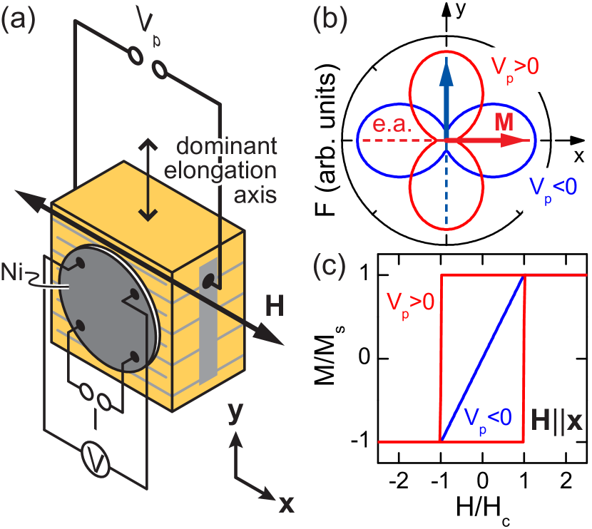
Figure 1: (a) Schematic illustration of the ferromagnetic thin film/actuator hybrid, indicating the orientation of the external magnetic field $\mathbf{H}\parallel\mathbf{x}$ and the contact scheme in four-point geometry for AMR measurements. (b) Free energy density contours in the $\mathbf{x}-\mathbf{y}$ film plane for different $V_{\mathrm{p}}$ applied, with the orientation of the magnetic easy axis (e.a.) depicted by the dashed lines. Thus, the equilibrium magnetization orientation is oriented along $\mathbf{x}$ for $V_{\mathrm{p}}>0\,\mathrm{V}$ (red line), while it is aligned along $\mathbf{y}$ for $V_{\mathrm{p}}<0\,\mathrm{V}$ (blue line). (c) Calculated $M\left(H\right)=\left(\mathbf{M}\cdot\mathbf{x}\right)/M_{\mathrm{s}}$ loops with $\mathbf{H}\parallel\mathbf{x}$ using a single-domain Stoner-Wohlfarth model, as explained in the text. In accordance to (b), the $M\left(H\right)$ curves show a magnetically easy $\mathbf{x}$ direction by the rectangular-shaped loop for $V_{\mathrm{p}}>0\,\mathrm{V}$ (red line), while the non-hysteretic line indicates a magnetically hard direction for $V_{\mathrm{p}}<0\,\mathrm{V}$ (blue line).

We realize a voltage control of magnetization in ferromagnetic thin film/piezoelectric actuator hybrid structures. The commercially available, co-fired $\mathrm{Pb}\left(\mathrm{Zr}_{x}\mathrm{Ti}_{1-x}\right)\mathrm{O}_{3}$ (PZT) piezoelectric multilayer stack actuators “PSt $150/2\times 3/5$” (Piezomechanik München) [Fig. 1(a)] comprise an interdigitated approx. $100\,\mathrm{\mu m}$ thick PZT-ceramic/AgPd electrode layer structure. For the ferromagnet, we use polycrystalline nickel (Ni) as a generic itinerant 3d magnet with a Curie temperature $T_{\mathrm{C}}>600\,\mathrm{K}$ (Ref. Leger et al., 1972) well above room temperature, a high bulk saturation magnetization $M_{\mathrm{s}}=493\,\mathrm{kA/m}$ (Ref. Pauthenet, 1982), a considerable polycrystalline volume magnetostriction $\bar{\lambda}=\frac{2}{5}\lambda_{100}+\frac{3}{5}\lambda_{111}=-32.9\times 10^{-6}$ (Ref. Lee, 1955), and a moderate anisotropic magnetoresistance (AMR) ratio $\Delta\rho/\rho_{0}=2\,\mathrm{\%}$ (Ref. McGuire and Potter, 1975). To allow for an optimized interfacial strain coupling between the assembled ferromagnetic and piezoelectric compounds, $100\,\mathrm{nm}$ thick Ni films were directly deposited onto an area of $3\,\mathrm{mm^{2}}$ on the actuators by electron beam evaporation at a base pressure of $7.0\times 10^{-8}\,\mathrm{mbar}$. The Ni films were covered in situ by $5\,\mathrm{nm}$ thick Au films to prevent oxidation. Prior to the evaporation process, a $140\,\mathrm{nm}$ thick polymethylmethacrylate (PMMA) layer was spin-coated onto the respective actuator face and baked at $110\,\mathrm{{}^{\circ}C}$ to electrically isolate the Ni film from the actuator electrodes.

As schematically sketched in Fig. 1(a), the actuator deforms upon the application of a voltage $V_{\mathrm{p}}\neq 0\,\mathrm{V}$, exhibiting a dominant elongation axis along $\mathbf{y}$ with a maximum strain $\epsilon_{y}=1.3\times 10^{-3}$ in the full voltage swing $-30\,\mathrm{V}\leq V_{\mathrm{p}}\leq+150\,\mathrm{V}$ (Ref. pie, 2010). Thus the ferromagnetic/piezoelectric hybrid allows to induce an electrically tunable strain in the Ni thin film. In particular, a voltage $V_{\mathrm{p}}>0\,\mathrm{V}$ ($V_{\mathrm{p}}<0\,\mathrm{V}$) results in an elongation with a related strain $\epsilon_{y}>0$ (contraction with $\epsilon_{y}<0$) along $\mathbf{y}$. Due to elasticity, such a tensile (compressive) strain along $\mathbf{y}$ is accompanied by a contraction (elongation) along the orthogonal in-plane direction $\mathbf{x}$, with about half the magnitude.

To quantify the effect of lateral elastic stress on the magnetic anisotropy of a ferromagnetic thin film, we rely on a magnetic free-energy model. Since this approach is discussed in detail, e.g., in Ref. Weiler et al., 2009, we here only qualitatively summarize our findings. Because we use polycrystalline ferromagnetic thin films, which exhibit no net crystalline magnetic anisotropy, only shape and strain-induced anisotropies need to be considered Bihler et al. (2008). The angular dependence of the total free energy density $F$ within the plane of such a uniaxially strained ferromagnetic film shows a $180^{\circ}$ periodicity, where maxima of $F$ correspond to magnetically hard directions, and accordingly minima to magnetically easy directions. In the Stoner-Wohlfarth (SW) model Stoner and Wohlfarth (1948), the magnetization orientation can be calculated from $F$, since in equilibrium $\mathbf{M}$ aligns along a local minimum of $F$. Regarding the in-plane magnetoelastic contribution to $F$ Chikazumi (1997)

$$F_{\textrm{me}}=\frac{3}{2}\bar{\lambda}\left(c_{12}-c_{11}\right)\left[\epsilon_{x}\left(\alpha_{x}^{2}-\frac{1}{3}\right)+\epsilon_{y}\left(\alpha_{y}^{2}-\frac{1}{3}\right)\right],$$ (1)

with the elastic stiffness constants $c_{ij}$ Lee (1955) and the direction cosines of the magnetization $\alpha_{x}$ and $\alpha_{y}$ with respect to $\mathbf{x}$ and $\mathbf{y}$, respectively, it is important to note that for nickel $\frac{3}{2}\bar{\lambda}\left(c_{12}-c_{11}\right)>0$. Therefore, in the absence of external magnetic fields, the magnetic easy axis is oriented parallel to compressive strain ($\epsilon<0$) and orthogonal to tensile strain ($\epsilon>0$). Consequently, an applied voltage $V_{\mathrm{p}}>0\,\mathrm{V}$ results in a magnetic easy axis and thus an equilibrium magnetization orientation along $\mathbf{x}$ [cf. red contour in Fig. 1(b)], while accordingly for $V_{\mathrm{p}}<0\,\mathrm{V}$ the magnetization is oriented along $\mathbf{y}$ [cf. blue contour in Fig. 1(b)]. Hence, we expect a $90^{\circ}$ rotation of the easy axis and thus the magnetization orientation upon inverting the polarity of $V_{\mathrm{p}}$.

Figure 1(c) shows calculated magnetization curves, normalized to the saturation magnetization $M_{\mathrm{s}}$, i.e., $M=\left(\mathbf{M}\cdot\mathbf{x}\right)/M_{\mathrm{s}}$, as a function of the external magnetic field magnitude $H$ at fixed voltages $V_{\mathrm{p}}$. The curves are calculated using a single-domain SW model for the external magnetic field $\mathbf{H}$ applied along $\mathbf{x}$ [cf. Fig. 1(a)], as this is the case for all experimental data presented below. The SW model relies on the coherent rotation of a single homogeneous magnetic domain (macrospin). For $V_{\mathrm{p}}>0\,\mathrm{V}$, the $\mathbf{x}$ direction coincides with the easy axis [e.a., see Fig. 1(b)] and thus the corresponding $M\left(H\right)$ loop [red curve in Fig. 1(c)] exhibits a rectangular, hysteretic shape Morrish (2001), which indicates an abrupt $180^{\circ}$ magnetization switching (i.e., a discontinuous magnetization reversal) at the coercive field $H_{\mathrm{c}}$. Contrarily, the $\mathbf{x}$ direction is magnetically hard for $V_{\mathrm{p}}<0\,\mathrm{V}$, and hence the blue magnetization curve in Fig. 1(c) exhibits no magnetic hysteresis as typically observed for hard-axis loops, which indicates a magnetization-reversal process via continuous rotation.

To determine the static magnetic properties of the Ni thin film/actuator hybrid, we employ spatially resolved magneto-optical Kerr effect (MOKE) imaging. More precisely, we perform longitudinal MOKE spectroscopy, which detects the projection $M=\mathbf{M}\cdot\mathbf{x}$ of the magnetization onto the magnetic field direction $\mathbf{H}\parallel\mathbf{x}$. All data were recorded at room temperature. Our MOKE setup is equipped with a high power red light emitting diode (center wavelength $\lambda=627\,\mathrm{nm}$). A slit aperture and a Glan Thompson polarizing prism yield an illumination path with $s$-polarized incident light. After reflecting off the sample, the light passes through a quarter wave plate to remove the ellipticity, and then transmits through a second Glan Thompson polarizing prism close to extinction serving as the analyzer. The Kerr signal is then focused by an objective lens and recorded with a CCD camera with a pixel size of $10\,\mathrm{\mu m}\times 10\,\mathrm{\mu m}$. While the setup has a rather low spatial resolution of several micrometers, it allows to image samples with lateral dimensions of several $\mathrm{mm^{2}}$ in a single-shot experiment. Such a large field of view is mandatory to investigate the piezo-induced $\mathbf{M}\left(V_{\mathrm{p}}\right)$, since the actuator electrodes are about $10\,\mathrm{\mu m}$ wide, and the active piezoelectric regions are about $100\,\mathrm{\mu m}$ wide.

To enable AMR measurements simultaneously to MOKE, we contacted the Ni film on top in four-point geometry [see Fig. 1(a)]. All AMR data shown in the following were recorded with a constant bias current $\mathbf{I}$ parallel to $\mathbf{H}\parallel\mathbf{x}$. The longitudinal resistance in a single-domain model is given by McGuire and Potter (1975)

$$R=R_{\perp}+\left(R_{\parallel}-R_{\perp}\right)\cos^{2}\beta,$$ (2)

where $\beta$ is the angle between $\mathbf{M}$ and $\mathbf{I}$, and $R_{\perp}$ and $R_{\parallel}$ are the resistances at $\mathbf{I}\perp\mathbf{M}$ and $\mathbf{I}\parallel\mathbf{M}$, respectively.

As discussed in more detail in the results section, we apply several image-processing procedures to extract the relevant magnetic information. On the one hand, we use the difference-image technique, i.e., the digital subtraction of two images, to enhance the magneto-optical contrast and to exclude any non-magnetic signal contributions. To this end, a reference image is recorded in a magnetically saturated state and subtracted from subsequent images Schmidt et al. (1985). On the other hand, for a quantitative magnetization analysis we normalize the observed image contrast. To this end, we define a region of interest (ROI), which corresponds to the region covered with Ni. Within this ROI, we integrate over all pixels of the CCD-camera image and normalize the resulting value with respect to the ones related to the two opposite single-domain saturation states. This evaluation yields an effective averaged magnetization $-1\leq M/M_{\mathrm{s}}\leq 1$. The latter can be considered as an effective macrospin, in which any microscopic magnetic texture has been averaged out. It will be referred to as “integrated MOKE loop” in the following.

III Results and discussion

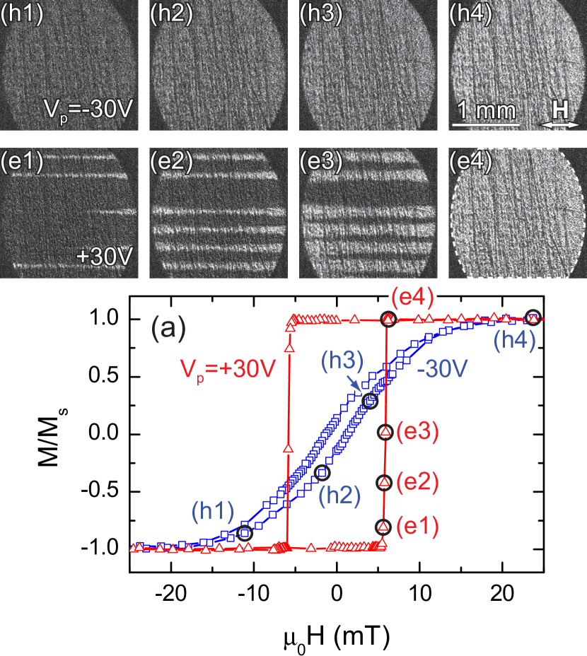
Figure 2: Magnetic domain evolution as a function of the external magnetic field magnitude. For $V_{\mathrm{p}}=-30\,\mathrm{V}$, the magnetic hard axis is along $\mathbf{H}\parallel\mathbf{x}$, while for $V_{\mathrm{p}}=+30\,\mathrm{V}$, the easy axis is along $\mathbf{H}\parallel\mathbf{x}$. (a) Integrated MOKE $M\left(H\right)$ loops for $V_{\mathrm{p}}=-30\,\mathrm{V}$ (open blue squares) and $V_{\mathrm{p}}=+30\,\mathrm{V}$ (open red triangles), using the region of interest depicted by the dashed white contour in (e4). The lines are guides to the eye. The open black circles mark the magnetic fields at which the MOKE images (h1)–(h4) and (e1)–(e4) were taken. Hereby, (h1)–(h4) were recorded for $V_{\mathrm{p}}=-30\,\mathrm{V}$ ($\mathbf{H}$ parallel to the magnetic hard axis) and (e1)–(e4) were recorded for $V_{\mathrm{p}}=+30\,\mathrm{V}$ ($\mathbf{H}$ parallel to the easy axis).

In a first series of experiments, we studied the magnetic domain evolution at constant strain, i.e., we recorded MOKE images at constant voltages $V_{\mathrm{p}}$ as a function of the external magnetic field magnitude $H$ for fixed magnetic field orientation $\mathbf{H}\parallel\mathbf{x}$. We refer to these experiments as $M\left(H\right)$ measurements. We applied a fixed voltage $V_{\mathrm{p}}$ to the actuator, swept the magnetic field to $\mu_{0}H=-50\,\mathrm{mT}$ to prepare the magnetization in a single-domain, negative saturation state, and acquired a reference image. Subsequently, the magnetic field was increased in steps, and a MOKE image was recorded at every field value. The corresponding domain evolution (obtained after subtraction of the reference image) and the integrated MOKE loops for $V_{\mathrm{p}}=-30\,\mathrm{V}$ and $V_{\mathrm{p}}=+30\,\mathrm{V}$ are shown in Fig. 2. The integrated MOKE loops in Fig. 2(a) clearly resemble the SW simulations in Fig. 1(c), such that at $V_{\mathrm{p}}=-30\,\mathrm{V}$ we obtain a smooth and continuous $M\left(H\right)$ loop for a magnetic hard axis along $\mathbf{H}\parallel\mathbf{x}$ (open blue squares), while $V_{\mathrm{p}}=+30\,\mathrm{V}$ yields a magnetic easy axis along $\mathbf{x}$ and thus results in a rectangular-shaped $M\left(H\right)$ loop with discontinuous magnetization-reversal processes (open red triangles).

We start the discussion with the data recorded at $V_{\mathrm{p}}=-30\,\mathrm{V}$, i.e., for a magnetic hard axis along $\mathbf{x}$. Figures 2(h1)–(h4) show MOKE images for an upsweep of the external magnetic field obtained at magnetic field values $\mathrm{h1}=-10.5\,\mathrm{mT}$, $\mathrm{h2}=-1.5\,\mathrm{mT}$, $\mathrm{h3}=4.0\,\mathrm{mT}$, and $\mathrm{h4}=23.0\,\mathrm{mT}$, marked by circles in the corresponding $M\left(H\right)$ loop presented graphically by square symbols in Fig. 2(a). In Figs. 2(h1)–(h4), the spatially resolved MOKE intensity is homogeneous over the whole Ni film, continuously changing from black to white with increasing magnetic field strength from negative to positive saturation. Hence, the sample is uniformly magnetized throughout the magnetization-reversal process, suggesting coherent and continuous magnetization rotation. Clearly, a single-domain SW approach is appropriate to model this behavior. In contrast, the magnetization reversal along the magnetic easy axis at $V_{\mathrm{p}}=+30\,\mathrm{V}$ is depicted in Figs. 2(e1)–(e4) at magnetic fields close to the coercive field [cf. $M\left(H\right)$ loop shown by open red triangles in Fig. 2(a)]. As apparent, magnetic domains nucleate and gradually propagate until the magnetization-reversal process is finally complete in Fig. 2(e4). For such a domain-driven magnetization-reversal process the simple SW single macrospin approach appears inadequate, since the magnetization-reversal process in $M\left(H\right)$ measurements is usually modeled by combining coherent rotation and domain-wall nucleation and/or unpinning Florczak and Dahlberg (1991). More precisely, in ferromagnetic thin films with uniaxial anisotropy, a magnetic-field induced magnetization reversal is determined by coherent rotation when the external magnetic field is oriented close to the magnetic hard axis, which is thus in good agreement with the SW model. In contrast, when the magnetic field is oriented along the magnetic easy axis, the abrupt magnetization reversal is caused by domain-wall effects, and thus proceeds via noncoherent switching. For other orientations, the magnetization first continuously reorients by coherent rotation, and then switches discontinuously and noncoherently (for details, see, e.g., Ref. Yan et al., 2001). In other words, in view of the domain pattern in Figs. 2(e1)–(e4), the macrospin model used in the literature for the magnetization reorientation $M\left(E\right)$ as a function of electric field at fixed external magnetic field magnitude Weiler et al. (2009) only represents a first-order approximation.

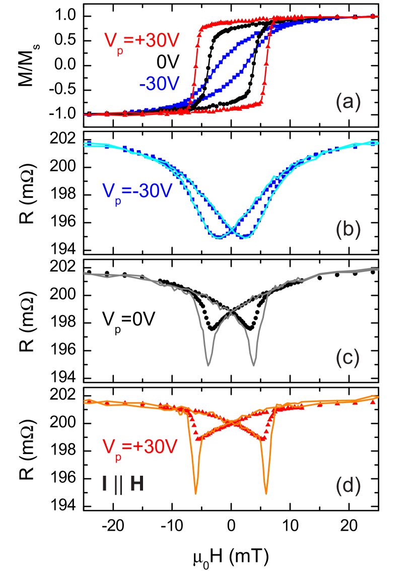
Figure 3: (a) Integrated MOKE $M\left(H\right)$ loops for $V_{\mathrm{p}}=-30\,\mathrm{V}$ (blue squares), $V_{\mathrm{p}}=0\,\mathrm{V}$ (black circles), and $V_{\mathrm{p}}=+30\,\mathrm{V}$ (red triangles). Simultaneously measured (full symbols) and simulated (solid lines) AMR $R\left(H\right)$ loops for $V_{\mathrm{p}}=-30\,\mathrm{V}$ (b), $V_{\mathrm{p}}=0\,\mathrm{V}$ (c), and $V_{\mathrm{p}}=+30\,\mathrm{V}$ (d). Apart from deviations in the vicinity of the coercive fields for $V_{\mathrm{p}}=0\,\mathrm{V}$ and $V_{\mathrm{p}}=+30\,\mathrm{V}$, the simulations based on a pseudo-macrospin model are in very good agreement with the measurements.

To examine the validity and limitations of the macrospin model for $M\left(E\right)$ in more detail, we now address the AMR recorded simultaneously to the MOKE data, referred to as $R\left(H\right)$ measurements. Figure 3(a) again depicts integrated MOKE loops along a magnetic hard axis ($V_{\mathrm{p}}=-30\,\mathrm{V}$, full blue squares), with zero applied stress ($V_{\mathrm{p}}=0\,\mathrm{V}$, full black circles), and along a magnetic easy axis ($V_{\mathrm{p}}=+30\,\mathrm{V}$, full red triangles). The corresponding AMR loops, represented by full symbols, are shown in Figs. 3(b), (c), and (d) for $V_{\mathrm{p}}=-30\,\mathrm{V}$, $V_{\mathrm{p}}=0\,\mathrm{V}$, and $V_{\mathrm{p}}=+30\,\mathrm{V}$, respectively. To quantitatively simulate the evolution of $R\left(H\right)$ in a macrospin-type SW model, we determined an effective, average magnetization orientation $\beta$ from the $M\left(H\right)$ loops in Fig. 3(a) via $\cos\beta=M/M_{\mathrm{s}}$ (cf. Ref. Brandlmaier et al., 2011). To this end, we use the effective, averaged magnetization orientation in the ROI as a pseudo-macrospin. It should be emphasized at this point that this pseudo-macrospin corresponds to a magnetization orientation $\beta$ averaged over differently oriented magnetic domains, see Figs. 2(e1)–(e4). Equation (2) with $R_{\parallel}=201.9\,\mathrm{m\Omega}$ and $R_{\perp}=194.9\,\mathrm{m\Omega}$ then yields the solid lines in Figs. 3(b), (c), and (d). As evident from the figure, the AMR calculated using the macrospin model accurately reproduces the measured AMR for $\mathbf{H}$ parallel to a hard axis ($V_{\mathrm{p}}=-30\,\mathrm{V}$). For $V_{\mathrm{p}}=0\,\mathrm{V}$ and $V_{\mathrm{p}}=+30\,\mathrm{V}$, $\mathbf{H}$ is along an axis with increasingly easy character and we observe an increasing deviation of the AMR simulation from the AMR experiment—however only for $H$ in the vicinity of the coercive fields [see Figs. 3(c) and (d)]. Hence, the AMR experiments corroborate the notion that the pseudo-macrospin is not adequate in the case of substantial microscopic domain formation, i.e., close to the coercive fields. Interestingly, however, the simulations yield very good agreement with the experimental results for all other magnetic field values. In summary, the magnetization reversal at constant strain in our multifunctional hybrid systems can be modeled in very good approximation using a pseudo-macrospin type of approach, except for a small range around $H\approx H_{\mathrm{c}}$ with substantial domain formation.

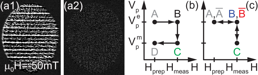
Figure 4: (a) Elastic strain-induced Kerr contrast patterns, recorded with the Ni film magnetized to saturation via the application of $\mu_{0}H=-50\,\mathrm{mT}$ at $V_{\mathrm{p}}=+30\,\mathrm{V}$. (a1) Difference image after a sweep to $V_{\mathrm{p}}=-30\,\mathrm{V}$ and (a2) back to $V_{\mathrm{p}}=+30\,\mathrm{V}$. (b), (c) Schematic illustrations of measurement sequences used to record magnetic Kerr images as a function of $V_{\mathrm{p}}$ without the strain-induced signal contributions.

In a second set of experiments we address the voltage control of the magnetization orientation. To this end, we record MOKE images and the AMR as a function of the voltage $V_{\mathrm{p}}$ at constant external magnetic bias field $\mathbf{H}$. However, it turns out that the different strain states at different $V_{\mathrm{p}}$ also give raise to a Kerr signal, as illustrated in Fig. 4. In these experiments, we aligned a magnetic easy axis along $\mathbf{H}\parallel\mathbf{x}$ by applying $V_{\mathrm{p}}=+30\,\mathrm{V}$, and initially magnetized the sample to saturation in a single-domain state by sweeping the magnetic field to $\mu_{0}H=-50\,\mathrm{mT}$. After recording a reference image, we swept the voltage to $V_{\mathrm{p}}=-30\,\mathrm{V}$, keeping $\mu_{0}H=-50\,\mathrm{mT}$ constant. Figure 4(a1) shows the difference image at $V_{\mathrm{p}}=-30\,\mathrm{V}$ with respect to the reference at $V_{\mathrm{p}}=+30\,\mathrm{V}$. After sweeping the voltage back to $V_{\mathrm{p}}=+30\,\mathrm{V}$, the Kerr difference contrast pattern completely vanishes [Fig. 4(a2)], indicating the reversibility of this process. Evidently, the observed Kerr contrast cannot be of magnetic origin, since the magnetic field $\mu_{0}H=-50\,\mathrm{mT}$ is way large enough to ensure magnetic saturation at any $V_{\mathrm{p}}$, such that neither the magnetization orientation nor the magnitude are subject to magnetoelastic modifications. The Kerr contrast thus must be of non-magnetic origin. Two mechanisms may account for these strain-induced contrast changes. First, the Poisson ratios of the PZT piezoelectric layers and the interdigitated electrodes differ. Thus, the strain induced by $V_{\mathrm{p}}\neq 0\,\mathrm{V}$ will be slightly inhomogeneous in the $\mathbf{x}-\mathbf{y}$ plane of the actuator, leading to local surface corrugations above the electrodes and thus to a modified intensity of the reflected light. Second, the PMMA layer in between piezo and Ni exhibits strain-induced birefringence, e.g., photoelastic birefringence Ohkita et al. (2005), which also results in a Kerr contrast.

To nevertheless extract the magnetic Kerr signal contributions, we apply two more elaborate measurement sequences. The basic sequence is schematically illustrated in Fig. 4(b). We magnetize the sample to a single-domain state by applying a magnetic preparation field $\mu_{0}H_{\mathrm{prep}}=-50\,\mathrm{mT}$ well exceeding the saturation field along the easy axis at $V_{\mathrm{p}}^{\mathrm{e}}=+30\,\mathrm{V}$ (point $\mathrm{A}$), then sweep the magnetic field to the measurement bias field $H_{\mathrm{meas}}$ (point $\mathrm{B}$), in turn sweep the voltage to the measurement voltage $V_{\mathrm{p}}^{\mathrm{m}}$ (point $\mathrm{C}$), and finally go back to the preparation field $H_{\mathrm{prep}}$ (point $\mathrm{D}$). A Kerr image is acquired at each point. Subsequently, we subtract the images corresponding to equal strain states, such that the resulting images $\mathrm{B}-\mathrm{A}$ and $\mathrm{C}-\mathrm{D}$ exhibit only contrast of magnetic origin. Hence, this procedure allows to image the evolution of $\mathbf{M}$ as a function of strain. To also investigate the reversibility of the voltage-induced magnetization changes, we modify the sequence as sketched in Fig. 4(c). After sweeping the voltage to the measurement voltage $V_{\mathrm{p}}^{\mathrm{m}}$ (point $\mathrm{C}$), it is cycled back to $V_{\mathrm{p}}^{\mathrm{e}}=+30\,\mathrm{V}$ (point $\overline{\mathrm{B}}$), and finally the magnetic field is returned to $H_{\mathrm{prep}}$ (point $\overline{\mathrm{A}}$). The difference images $\mathrm{B}-\mathrm{A}$ and $\overline{\mathrm{B}}-\overline{\mathrm{A}}$ then reveal the degree of reversibility.

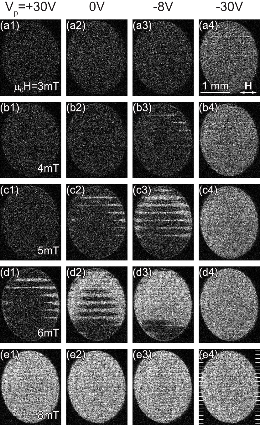
Figure 5: Evolution of the magnetization reorientation as a function of the voltage $V_{\mathrm{p}}$ at different, fixed magnetic bias fields after preparing a magnetic single-domain state at $\mu_{0}H_{\mathrm{prep}}=-50\,\mathrm{mT}$. The magnetic Kerr images are obtained using the sequence depicted in Fig. 4(b) (images in the first column show difference images $\mathrm{B}-\mathrm{A}$, all other images show difference images $\mathrm{C}-\mathrm{D}$). In the vicinity of the coercive field [$\mu_{0}H_{\mathrm{c}}\approx 6\,\mathrm{mT}$ at $V_{\mathrm{p}}=+30\,\mathrm{V}$, cf. Fig. 3(a)] for $\mu_{0}H_{\mathrm{meas}}=4\,\mathrm{mT}$ [(b1)–(b4)], $5\,\mathrm{mT}$ [(c1)–(c4)], and $6\,\mathrm{mT}$ [(d1)–(d4)], the voltage-controlled magnetization-reorientation process evidently occurs via magnetic domain nucleation and propagation, and finally attains a single-domain state at $V_{\mathrm{p}}=-30\,\mathrm{V}$. For other magnetic field strengths, e.g., $\mu_{0}H_{\mathrm{meas}}=3\,\mathrm{mT}$ [(a1)–(a4)] and $\mu_{0}H_{\mathrm{meas}}=8\,\mathrm{mT}$ [(e1)–(e4)], the Kerr image contrast changes homogeneously as a function of $V_{\mathrm{p}}$, i.e., the magnetization rotates coherently during the $V_{\mathrm{p}}$ sweep. The white lines in (e4) indicate the position of the actuator electrodes.

Figure 5 shows the magnetic Kerr images obtained using the sequence depicted in Fig. 4(b) as a function of the voltage $V_{\mathrm{p}}$ at different fixed magnetic bias fields $\mu_{0}H_{\mathrm{meas}}=3\,\mathrm{mT}$, $4\,\mathrm{mT}$, $5\,\mathrm{mT}$, $6\,\mathrm{mT}$, and $8\,\mathrm{mT}$, depicted in Figs. 5(a1)–(a4), (b1)–(b4), (c1)–(c4), (d1)–(d4), and (e1)–(e4), respectively. Hereby, the images (a)–(c) are recorded slightly below the coercive field, while (d) ($\mu_{0}H_{\mathrm{meas}}=6\,\mathrm{mT}$) is directly at the coercive field [$\mu_{0}H_{\mathrm{c}}\approx 6\,\mathrm{mT}$ at $V_{\mathrm{p}}=+30\,\mathrm{V}$, cf. Fig. 3(a)]. For the latter [Fig. 5(d1)], domain nucleation already starts without changing $V_{\mathrm{p}}$. The difference images $\mathrm{B}-\mathrm{A}$ shown in the first column of Fig. 5 are acquired at the preparation voltage $V_{\mathrm{p}}^{\mathrm{e}}=+30\,\mathrm{V}$ after a magnetic field sweep from $\mu_{0}H_{\mathrm{prep}}=-50\,\mathrm{mT}$ to the bias field $H_{\mathrm{meas}}$. The difference images $\mathrm{C}-\mathrm{D}$ in the latter three columns result from a consecutive application of the measurement sequence with different measurement voltages $V_{\mathrm{p}}^{\mathrm{m}}=0\,\mathrm{V}$, $-8\,\mathrm{V}$, and $-30\,\mathrm{V}$. As evident from Figs. 5(a1), (b1), and (c1), no magnetic contrast is yet visible at $H_{\mathrm{meas}}$, indicating a uniform, single-domain magnetization along the initial magnetic field orientation $\mu_{0}H_{\mathrm{prep}}<0\,\mathrm{mT}$, i.e., antiparallel to the bias magnetic field orientation $\mu_{0}H_{\mathrm{meas}}>0\,\mathrm{mT}$. Upon gradually decreasing $V_{\mathrm{p}}$, a noncoherent magnetization-reorientation process sets in for magnetic fields close to the coercive field [see Figs. 5(b3) and (c2)] via magnetic domain nucleation and propagation, until the process is complete at $V_{\mathrm{p}}=-30\,\mathrm{V}$, as shown in the images in the last column. We note that the domain nucleation preferably proceeds on top of the electrodes, which we attribute to the slight strain inhomogeneities discussed in the context of Fig. 4(a1). The final image contrast after the magnetization reorientation is homogeneously white [Figs. 5(a4) to (e4)], evidencing a magnetic single-domain state.

Figures 5(a1)–(a4), (b1)–(b4), (c1)–(c4), and (e1)–(e4) show a fully voltage-controlled magnetization reorientation from an initial magnetic single-domain state to a final single-domain state. As apparent from the Kerr images in Fig. 5, for externally applied magnetic fields close to $H_{\mathrm{c}}$ the magnetization-reorientation process evolves via domain nucleation and propagation. In contrast, for other magnetic field strengths [$\mu_{0}H_{\mathrm{meas}}<4\,\mathrm{mT}$ and $\mu_{0}H_{\mathrm{meas}}>7\,\mathrm{mT}$, see Figures 5(a1)–(a4) and (e1)–(e4)]) the Kerr image contrast changes homogeneously as a function of $V_{\mathrm{p}}$, i.e., the magnetization rotates coherently during the $V_{\mathrm{p}}$ sweep.

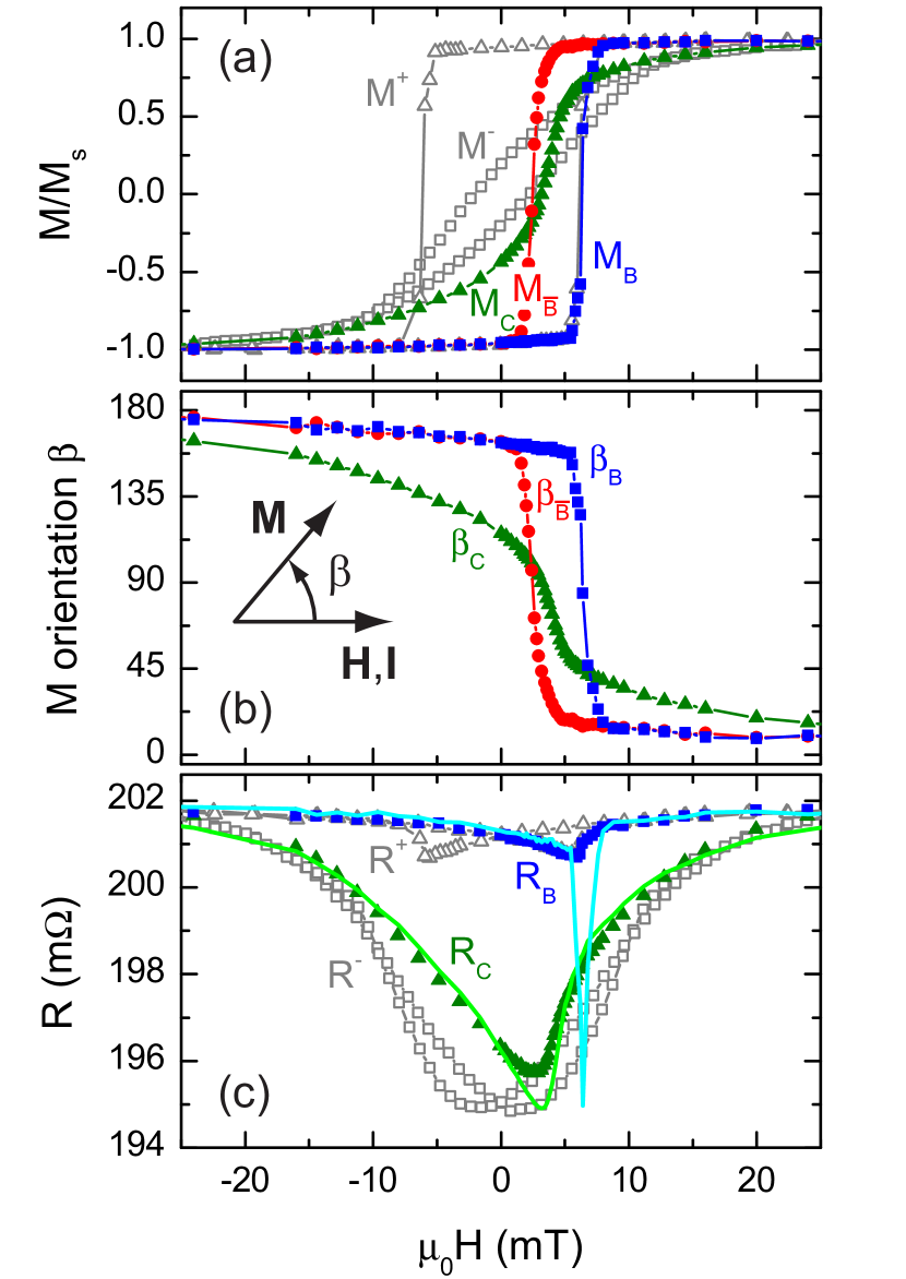
Figure 6: Voltage-dependent $M$ and $R$ measurements. The panels show data acquired at the points $\mathrm{B}$ (full blue squares), $\overline{\mathrm{B}}$ (full red circles), and $\mathrm{C}$ (full green triangles) as a function of the measurement field $H=H_{\mathrm{meas}}$ in the sequences depicted in Figs. 4(b) and (c). (a) Integrated MOKE $M\left(V_{\mathrm{p}}\right)$ curves obtained from the respective difference images. For comparison, the open gray squares and open gray triangles depict the $M\left(H\right)$ loops for $V_{\mathrm{p}}=-30\,\mathrm{V}$ ($\mathrm{M}^{-}$) and $+30\,\mathrm{V}$ ($\mathrm{M}^{+}$), respectively. (b) Macrospin magnetization orientation $\beta$ with the angle $\beta$ between $\mathbf{M}$ and $\mathbf{I}$, calculated from the measured data displayed in (a) using the pseudo-macrospin model. (c) Corresponding AMR $R\left(V_{\mathrm{p}}\right)$ curves (symbols) and simulations (lines) using the simultaneously recorded $M\left(V_{\mathrm{p}}\right)$ curves [(a) and (b)] and the AMR parameters given in the text showing very good overall agreement with the experiment. Hereby, the blue and green solid lines illustrate the simulated evolution of $R_{\mathrm{B}}\left(H\right)$ and $R_{\mathrm{C}}\left(H\right)$, respectively. In analogy to (a), the $R\left(H\right)$ loops for $V_{\mathrm{p}}=-30\,\mathrm{V}$ ($\mathrm{R}^{-}$) and $+30\,\mathrm{V}$ ($\mathrm{R}^{+}$) are additionally depicted by open gray squares and open gray triangles, respectively.

To quantitatively evaluate the Kerr images recorded as a function of $V_{\mathrm{p}}$, we finally test the applicability of a macrospin picture for the description of $M\left(V_{\mathrm{p}}\right)$, and address the reversibility of the voltage-induced magnetization reorientation. To this end, we consecutively applied the two measurement sequences illustrated in Figs. 4(b) and (c) with different measurement bias fields $H_{\mathrm{meas}}$. More precisely, for each $H_{\mathrm{meas}}$ we first applied the basic sequence shown in Fig. 4(b) with $\mu_{0}H_{\mathrm{prep}}=-50\,\mathrm{mT}$, $V_{\mathrm{p}}^{\mathrm{e}}=+30\,\mathrm{V}$, and $V_{\mathrm{p}}^{\mathrm{m}}=-30\,\mathrm{V}$. Then we applied the modified sequence shown in Fig. 4(c) at the same $H_{\mathrm{meas}}$. At each point, a Kerr image is acquired and the resistance is recorded. We refer to these experiments as $M\left(V_{\mathrm{p}}\right)$ and $R\left(V_{\mathrm{p}}\right)$ measurements, respectively. The evolution of the corresponding integrated MOKE $M\left(V_{\mathrm{p}}\right)$ signals obtained from the difference images $\mathrm{B}-\mathrm{A}$, $\overline{\mathrm{B}}-\overline{\mathrm{A}}$, and $\mathrm{C}-\mathrm{D}$ as a function of the measurement field $H=H_{\mathrm{meas}}$ is shown in Fig. 6(a) and referred to as $M_{\mathrm{B}}\left(H\right)$ (full blue squares), $M_{\overline{\mathrm{B}}}\left(H\right)$ (full red circles), and $M_{\mathrm{C}}\left(H\right)$ (full green triangles), respectively. We again determined the magnetization orientation $\beta$ in a macrospin approximation, as displayed in Fig. 6(b). The corresponding AMR $R\left(V_{\mathrm{p}}\right)$ curves simultaneously measured with the Kerr images at the points $\mathrm{B}$ and $\mathrm{C}$ are depicted in Fig. 6(c) by full blue squares and full green triangles and referred to as $R_{\mathrm{B}}\left(H\right)$ and $R_{\mathrm{C}}\left(H\right)$, respectively. For comparison, we also included the integrated MOKE $M\left(H\right)$ and AMR $R\left(H\right)$ data recorded as a function of the external magnetic field at constant $V_{\mathrm{p}}=-30\,\mathrm{V}$ and $+30\,\mathrm{V}$ as open gray squares [denoted as $\mathrm{M}^{-}$ and $\mathrm{R}^{-}$ in Figs. 6(a) and (c), respectively] and open gray triangles ($\mathrm{M}^{+}$ and $\mathrm{R}^{+}$), respectively.

Using the $M_{\mathrm{B}}\left(H\right)$ and $M_{\mathrm{C}}\left(H\right)$ curves [Fig. 6(a)] recorded simultaneously with $R_{\mathrm{B}}\left(H\right)$ and $R_{\mathrm{C}}\left(H\right)$, respectively, we again simulate the AMR with Eq. (2) and the values of the parameters $R_{\parallel}$ and $R_{\perp}$ given above. The AMR curves thus calculated for $R_{\mathrm{B}}\left(H\right)$ and $R_{\mathrm{C}}\left(H\right)$ are displayed by the solid blue and green lines in Fig. 6(c), respectively. Evidently, the measurement and simulation for both $R_{\mathrm{B}}\left(H\right)$ and $R_{\mathrm{C}}\left(H\right)$ are in very good agreement, with the exception of a narrow region around $H_{\mathrm{c}}$, where the macrospin model fails to adequately describe the experiment, in full consistency with the above findings for $M\left(H\right)$ and $R\left(H\right)$ measurements (cf. Fig. 3). Therefore, except for a small magnetic-field range close to $H_{\mathrm{c}}$ we can describe the voltage-induced magnetization changes in very good approximation in a simple macrospin model.

As we now have demonstrated the validity of the macrospin approach also for the description of $M\left(V_{\mathrm{p}}\right)$ and $R\left(V_{\mathrm{p}}\right)$ measurements, we can consistently model the evolution of the magnetization orientation as a function of the voltage $V_{\mathrm{p}}$ and the external magnetic field $H$ (Fig. 6). We start the discussion with the evolution of $M_{\mathrm{B}}\left(H\right)$ [full blue squares in Fig. 6(a)], which coincides with the $M\left(H\right)$ loop recorded at $V_{\mathrm{p}}=+30\,\mathrm{V}$. The corresponding macrospin magnetization orientation $\beta_{\mathrm{B}}$ is initially aligned along $180^{\circ}$ for large negative external magnetic field [full blue squares in Fig. 6(b)], continuously rotates to $\approx 160^{\circ}$ with increasing magnetic field strength, then abruptly switches into a direction close to $\beta_{\mathrm{B}}=0^{\circ}$ at the magnetic coercive field, and then continuously rotates towards $0^{\circ}$, the orientation of the external magnetic field. For external magnetic measurement fields $\mu_{0}H_{\mathrm{meas}}\lesssim 0\,\mathrm{mT}$, the influence of the Zeeman contribution to the total free energy density in the film plane $F=F_{\mathrm{Zeeman}}+F_{\textrm{me}}$ decreases with decreasing absolute value of the external magnetic field, which results in an increasingly dominating magnetoelastic anisotropy contribution. Hence, the magnetization orientation cannot be modified at $\mu_{0}H_{\mathrm{prep}}=-50\,\mathrm{mT}$ by application of $V_{\mathrm{p}}$ and can be increasingly rotated to about $\Delta\beta=50^{\circ}$ at $\mu_{0}H=0\,\mathrm{mT}$ by changing $V_{\mathrm{p}}=+30\,\mathrm{V}\rightarrow-30\,\mathrm{V}$ [$\beta_{\mathrm{B}}\left(\mu_{0}H=0\,\mathrm{mT}\right)\approx 165^{\circ}$ and $\beta_{\mathrm{C}}\left(\mu_{0}H=0\,\mathrm{mT}\right)\approx 115^{\circ}$]. In this magnetic field range, $M_{\mathrm{B}}\left(H\right)$ and $M_{\overline{\mathrm{B}}}\left(H\right)$ fully coincide ($\mathbf{M}_{\mathrm{B}}\parallel\mathbf{M}_{\overline{\mathrm{B}}}$), i.e., the voltage-induced magnetization reorientation is fully reversible. We would like to emphasize that this implies a continuous and reversible magnetization rotation at zero external magnetic field, solely via application of appropriate voltages $V_{\mathrm{p}}$ to the piezoelectric actuator. In the second field range $0\,\mathrm{mT}\lesssim\mu_{0}H_{\mathrm{meas}}\lesssim 8\,\mathrm{mT}$ in Fig. 6, the angular range within which the magnetization orientation can be rotated by changing $V_{\mathrm{p}}=+30\,\mathrm{V}\rightarrow-30\,\mathrm{V}$ continuously increases, but the magnetization reorientation is not reversible, since $M_{\mathrm{B}}\left(H\right)\neq M_{\overline{\mathrm{B}}}\left(H\right)$. This observation can also be consistently understood in a macrospin model. Here, $\mu_{0}H_{\mathrm{prep}}=-50\,\mathrm{mT}$ yields $\mathbf{M}_{\mathrm{B}}$ antiparallel to $\mu_{0}H_{\mathrm{meas}}>0\,\mathrm{mT}$ aligned along $0^{\circ}$, i.e., $\mathbf{M}_{\mathrm{B}}$ resides in a local minimum of $F$ at $V_{\mathrm{p}}=+30\,\mathrm{V}$ and thus in a metastable state. Sweeping $V_{\mathrm{p}}$ from $+30\,\mathrm{V}$ to $-30\,\mathrm{V}$ yields $\mathbf{M}_{\mathrm{C}}$ aligned along the global minimum of $F$. However, upon increasing the voltage back to $+30\,\mathrm{V}$, the magnetization does not rotate back in the same way, but evolves into the global minimum of $F$ close to $0^{\circ}$ (for details of the quantitative evolution of $F$ as a function of $V_{\mathrm{p}}$, see Ref. Weiler et al., 2009). Therefore, the voltage sweep $V_{\mathrm{p}}=+30\,\mathrm{V}\rightarrow-30\,\mathrm{V}\rightarrow+30\,\mathrm{V}$ results in an irreversible magnetization-orientation change with $\mathbf{M}_{\mathrm{B}}$ and $\mathbf{M}_{\overline{\mathrm{B}}}$ essentially being antiparallel at $V_{\mathrm{p}}=+30\,\mathrm{V}$. The third magnetic field range $\mu_{0}H_{\mathrm{meas}}\gtrsim 10\,\mathrm{mT}$ exceeds $\mu_{0}H_{\mathrm{c}}$ for $V_{\mathrm{p}}=+30\,\mathrm{V}$, resulting in a (nearly) parallel alignment of $\mathbf{H}_{\mathrm{meas}}$ and $\mathbf{M}_{\mathrm{B}}$. Here, the evolution of $M\left(V_{\mathrm{p}}\right)$ is analogous to the above described for $\mu_{0}H_{\mathrm{meas}}\lesssim 0\,\mathrm{mT}$, i.e., sweeping $V_{\mathrm{p}}=+30\,\mathrm{V}\rightarrow-30\,\mathrm{V}\rightarrow+30\,\mathrm{V}$ rotates $\mathbf{M}_{\mathrm{B}}$ to $\mathbf{M}_{\mathrm{C}}$ and back to $\mathbf{M}_{\mathrm{B}}\parallel\mathbf{M}_{\overline{\mathrm{B}}}$. The angle of rotation decreases with increasing magnetic field strength.

Overall, these findings demonstrate that the macrospin model cannot only be applied to describe the $M\left(H\right)$ and $R\left(H\right)$ measurements, but also to the $M\left(V_{\mathrm{p}}\right)$ and $R\left(V_{\mathrm{p}}\right)$ measurements—except for a narrow range around the coercive field.

IV Conclusion

In conclusion, we have studied the applicability and limitations of a Stoner-Wohlfarth type macrospin model for the description of changes in the magnetic configuration and magnetoresistance of ferromagnetic/ferroelectric hybrid systems. To this end, we investigated the magnetic properties in Ni thin film/piezoelectric actuator hybrids using simultaneous spatially resolved MOKE and integral magnetotransport measurements at room temperature. Using dedicated measurement sequences to suppress strain-induced contributions to the Kerr signal, the imaging of the magnetization state both as a function of magnetic field and electrical voltage applied to the piezoelectric actuator becomes possible. We extract an effective magnetization orientation (macrospin) by spatially averaging the Kerr images. For experiments both as a function of $H$ and of $V_{\mathrm{p}}$, we find very good agreement between the AMR calculated using the macrospin and the measured AMR. Our results show that the magnetization continuously reorients by coherent rotation—except for $\mathbf{H}$ along a magnetically easy direction in a very narrow region around the magnetic coercive field, where the magnetization reorientation dominantly evolves via domain nucleation and propagation. Taken together, on length scales much larger than the magnetic domain size, a SW type macrospin model for both $M\left(H\right)$ and $M\left(V_{\mathrm{p}}\right)$ adequately describes the corresponding $R\left(H\right)$ and $R\left(V_{\mathrm{p}}\right)$.