Integer quantum Hall effect in a square lattice revisited

Abstract

We investigate the phenomenon of integer quantum Hall effect in a square lattice, subjected to a perpendicular magnetic field, through Landauer-Büttiker formalism within the tight-binding framework. The oscillating nature of longitudinal resistance and near complete suppression of momentum relaxation processes are examined by studying the flow of charge current using Landauer-Keldysh prescription. Our analysis for the lattice model corroborates the finding obtained in the continuum model and provides a simple physical understanding.

I Introduction

The phenomenon of the integer quantum Hall effect (IQHE) is one of the most significant discoveries in condensed matter physics klit . At much low temperatures, typically below $1\,$K, this phenomenon occurs in two-dimensional ($2$D) electron systems in presence of a strong perpendicular magnetic field. It has been observed that the Hall resistance is quantized in units of $h/2e^{2}$ with a great accuracy, specified in parts per million, and due to this impressive accuracy it is utilized as a resistance standard hart . Such a precise quantization of the Hall resistance comes from almost complete suppression of momentum relaxation processes in the quantum Hall regime. In a finite width conductor at high magnetic fields, the states carrying current in one direction are spatially separated from those carrying currents in the opposite direction, and as a result the overlaps between these two groups of states get significantly reduced which results in a suppression of backscattering. The near complete suppression of backscattering between the forward and backward propagating states leads to a truly ballistic conductor even in the presence of impurities. The quantized nature of Hall resistance looks like the quantized resistance of conventional ballistic conductors, but in these conductors precise quantization cannot be achieved since the backscattering processes are not fully removed datta .

It has also been noticed that in a Hall bar the longitudinal resistance oscillates as a function of the Fermi energy $E_{F}$. Naturally it may occur to our mind that when the Fermi energy matches with anyone of the Landau levels i.e., with a peak in the density of states (DOS) profile, the resistance should have a minimum. But the real fact is completely opposite to that. The resistance becomes minimum whenever the Fermi energy lies between two Landau levels where the density of states also has a minimum, and, it leads to an immense curiosity and gives rise to the question about the current carrying states through the sample. It has been observed that the states those are situated near the edges of the sample, the so-called edge states, play an important role for carrying current when the longitudinal resistance has a minimum halp ; macd . It is quite surprising that at the minima, the longitudinal resistance is almost zero and the electrons are able to traverse a long distance without dissipating their momentum. It emphasizes that something special must be taking place which provide near complete suppression of the momentum relaxation processes in this regime.

Several studies already exist in the literature which deal with the quantized nature of the Hall resistance, oscillating behavior of the longitudinal resistance, existence of the edge

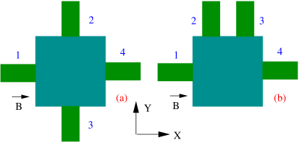
Figure 1: (Color online). Four probe set-ups for determining (a) the Hall resistance and (b) the longitudinal resistance.

states and almost complete suppression of the backscattering processes in a Hall bar based on the continuum model lau ; thou1 ; thou2 ; pran ; avr ; klit1 . However, no rigorous effort has been made so far, to the best of our knowledge, to unravel all these features within a discrete lattice model. In the present work we consider a two-dimensional square lattice in presence of a perpendicular magnetic field and establish them describing the system by the tight-binding (TB) model. Using the Landauer-Büttiker formalism datta we find the longitudinal and transverse conductivities. On the other hand, to investigate the behavior of the current carrying states when Fermi energy lies between two Landau levels or coincides with a Landau level we use Landauer-Keldysh prescription niko1 ; niko2 . From this study we can clearly describe the momentum relaxation processes. The physical picture about QHE that emerges from our present study based on the discrete lattice model of the Hall bar is exactly the same as obtained in the continuum model and provides much insight to the problem under realistic condition. This approach could be much more useful in further investigation of the unconventional quantum Hall effect in graphene where the Hall conductivity is half-integer quantized novo ; kim , showing plateaus at $\sigma_{xy}=(4e^{2}/h)(n+1/2)$, $n=0$, $\pm 1$, $\pm 2$, $\dots$, since this lattice model might be adapted with more convenience in graphene and other topologically insulating materials hata ; long . It is our first step towards this direction.

In what follows, we present the results. In Section $2$, we describe the model and theoretical formulation. Section $3$ contains the numerical results and related discussions, and we draw our conclusions in Section $4$.

II The model and Theoretical formulation

The quantum Hall system is shown schematically in Fig. 1, where a square lattice, placed in a magnetic field $\vec{B}$ perpendicular to its plane, is attached to four finite width leads. The TB Hamiltonian for a square lattice with $N$ atomic sites in both the $x$ and $y$ directions reads,

$$H = \sum_{m,n}\epsilon_{m,n}c_{m,n}^{{\dagger}}c_{m,n}+t\sum_{m,n}\left(c_{m+1,n}^{{\dagger}}c_{m,n}\right.$$ (1)

$$+ \left.c_{m,n+1}^{{\dagger}}c_{m,n}\,e^{i\theta_{m}}+\mbox{h.c.}\right).$$

Here $\epsilon_{m,n}$ represents the site energy of an electron at the lattice site ($m$,$n$), $m$ and $n$ being the $x$ and $y$ co-ordinates of the site, respectively. $c_{m,n}^{\dagger}$ ($c_{m,n}$) corresponds to the creation (annihilation) operator of an electron at the site ($m$,$n$) and $t$ is the nearest-neighbor hopping integral. The phase factor $\theta_{m}=2\pi mBa^{2}$ ($a$ being the lattice spacing) arises due to the magnetic field $B$ with the choice of the vector potential $A$$\,=$($0,Bx,0$).

The side-attached leads are taken as semi-infinite square lattice ribbons, which are also described by TB Hamiltonians similar to Eq. 1, where the hopping terms do not invoke the phase factor $e^{i\theta_{m}}$ since $\vec{B}=0$ in the leads. The lead Hamiltonians are parametrized by constant on-site potential $\epsilon_{0}$ and nearest-neighbor hopping strength $t_{0}$. The hopping integrals between the boundary sites of the leads and the quantum Hall system are parametrized by $\tau$. The number of sites in the transverse direction of the leads is denoted by $M_{y}$.

In order to find the Hall resistance using Landauer-Büttiker formalism, we connect the leads to the sample as prescribed in Fig. 1(a) and restrict ourselves within the coherent transport regime datta . The voltage leads, namely, lead-2 and lead-3 are attached on the opposite sides of the sample. In this formalism one can treat all the leads (i.e., current and voltage leads) on equal footing and express the current in the lead-p as $I_{p}=\sum_{q=1}^{4}G_{pq}\left[V_{p}-V_{q}\right]$, $G_{pq}$ being the conductance coefficient related to transmission coefficient $T_{pq}$ between the lead-p and lead-q by the expression $G_{pq}=(2e^{2}/h)T_{pq}$ (factor $2$ accounts for the spin of the electrons). Here $V_{p}$ is the applied bias voltage in the lead-p. Since the currents in the various leads depend only on voltage differences among them, we can set one of the voltages to zero without loss of generality. Here we set $V_{4}=0$. It allows us to write the currents in three other leads in the form of matrix equation, $V$=$\mathcal{G}$^-1$I$, where $\mathcal{G}$ is a $3\times 3$ matrix whose elements are expressed as follows: $\mathcal{G}_{ii}=\sum_{k}^{k\neq i}G_{ik}$ and $\mathcal{G}_{ij}=-G_{ij}$, where $k$ runs from $1$ to $4$. The above matrix equation simplifies in the form:

$$\left\{\begin{array}[]{c}V_{1}\\ V_{2}\\ V_{3}\\ \end{array}\right\}=\left\{\begin{array}[]{ccc}R_{11}&R_{12}&R_{13}\\ R_{21}&R_{22}&R_{23}\\ R_{31}&R_{32}&R_{33}\\ \end{array}\right\}\left\{\begin{array}[]{c}I_{1}\\ I_{2}\\ I_{3}\\ \end{array}\right\}$$ (2)

where, the matrix $R$ is the inverse of $\mathcal{G}$. In our four-terminal set-up (Fig. 1(a)) the Hall resistance is determined from the relation,

$$R_{H}=\left[\frac{V_{2}-V_{3}}{I_{1}}\right]_{I_{2}=I_{3}=0}=R_{21}-R_{31}.$$ (3)

On the other hand, to determine the longitudinal resistance we connect the leads to the conductor as shown in Fig. 1(b), attaching the voltage leads lead-2 and lead-3 on the same side of the conductor. For this set-up also the above expressions remain invariant, and the longitudinal resistance is given by $R_{L}=R_{21}-R_{31}$. Obviously, for this set-up the numerical values of $R_{21}$ and $R_{31}$ are different from those of the previous set-up (Fig. 1(a)).

With these $R_{L}$ and $R_{H}$ we can determine the longitudinal and Hall conductivities where the conductivity tensor $\sigma_{\mu\nu}$ is the inverse of the resistivity tensor $\rho_{\mu\nu}$. Mathematically it is expressed as $\sigma_{\mu\nu}=\left(\rho_{\mu\nu}\right)^{-1}$, in which $\rho_{xx}$ and $\rho_{xy}$ correspond to the longitudinal and Hall resistivities, respectively. For a square lattice, $\rho_{xx}=\rho_{yy}=R_{L}$ and $\rho_{xy}=-\rho_{yx}=R_{H}$. Therefore, we can write the final expressions of the conductivities as hajdu ,

$$\sigma_{xx}=\sigma_{yy}=\frac{R_{L}}{R_{L}^{2}+R_{H}^{2}};\,\sigma_{yx}=-\sigma_{xy}=\frac{R_{H}}{R_{L}^{2}+R_{H}^{2}}.$$ (4)

Next, we find the bond charge current between the atomic sites $n$ and $n^{\prime}$ by the Landauer-Keldysh method using the relation niko1 ; niko2 ,

$$\langle\hat{J}_{nn^{\prime}}\rangle=\frac{et}{h}\int\limits_{E_{F}-eV_{0}/2}^{E_{F}+eV_{0}/2}\mbox{Tr}_{s}\left[G_{nn^{\prime}}^{<}(E)-G_{n^{\prime}n}^{<}(E)\right]dE.$$ (5)

It actually describes the flow of charges which start at the site $n$ and end up at the site $n^{\prime}$. In this expression $G^{<}$ is the conventional lesser Green’s function niko1 and $V_{0}$ is the applied potential difference between the biased leads. Here trace Tr_s is performed in the spin Hilbert space, writing the Hamiltonian Eq. 1 including the spin of the electrons.

Throughout the numerical calculations we set $\epsilon_{0}=0$, lattice spacing $a=1$ and fix the hopping integrals ($t$, $t_{0}$ and $\tau$) at $1$. All energies are measured in units of $t$ and we choose $c=e=h=1$.

III Numerical results and discussion

In the left panel of Fig. 2 we show the quantized nature of the Hall conductance together with the density of states for an ordered ($W=0$, $W$ measures the disorder strength in the sample) square lattice. The sharp peaks in the DOS are associated with the Landau bands those are produced in the presence of magnetic field $B$. For a fixed sample size, the total number of Landau bands and the number of states in each band strongly depend on the strength of the applied magnetic field. Here we choose the uniform magnetic field $B$ in the form $1/Q$, $Q$ being an

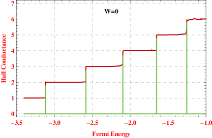
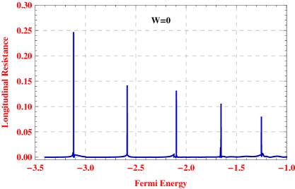
Figure 2: (Color online). Left panel: Hall conductance (red line) as a function of Fermi energy and the electronic density of states (green line) for a perfect ($W=0$) square lattice of size $20\times 20$ considering $B=0.05$. Right panel: Longitudinal resistance as a function of Fermi energy for the same parameter values.

integer, and it generates $Q$ number of Landau bands in the energy spectrum. This choice of the magnetic field makes each Landau band populated by $N^{2}/Q$ states for a square lattice of size $N\times N$. Thus, for the set of parameter values chosen in Fig. 2, we will get twenty Landau bands at the peaks of the DOS spectrum and each band accommodates twenty states. Since here we present the results only for a particular energy range, few Landau bands are visible. From the spectrum it is observed that the Hall conductance increases in discrete steps whenever the Fermi energy crosses peaks in the DOS profile. This is what we would expect from an ordinary ballistic waveguide where two-terminal conductance changes in integer steps associated with the integer number of sub-bands or transverse modes at the Fermi energy $E_{F}$ datta . On the other hand, plateaus appear in the Hall conductance when the Fermi energy lies between two Landau bands. At these plateaus the Hall conductance gets the value $(2e^{2}/h)M$, where $M$ corresponds to the total number of Landau bands below the Fermi energy. This is exactly equal to the number of edge states at the Fermi energy and these states play the equivalent role similar to the transverse modes in a conventional ballistic waveguide.

Though the quantized Hall conductance resembles to the quantized conductance in traditional ballistic waveguides, but the strange precise quantization can never be achieved in ordinary ballistic conductors since the backscattering processes are not fully suppressed. The almost complete elimination of the backscattering processes can only be achieved in the quantum Hall regime which provides surprisingly precise quantized Hall conductance. To reveal this fact, we examine the flow of charge current in a perfect conductor when the Fermi energy lies within a plateau region. The result is shown in the left panel of Fig. 3, where $E_{F}$ is set at $-2.8$, and it predicts that the charge current flows only through the edges of the conductor and no current is available in the bulk. Very nicely we notice that the states carrying current from the left side of the sample to the right one are spatially separated from those carrying current in the reverse direction. As a result the overlap between the forward and backward propagating states is almost reduced to

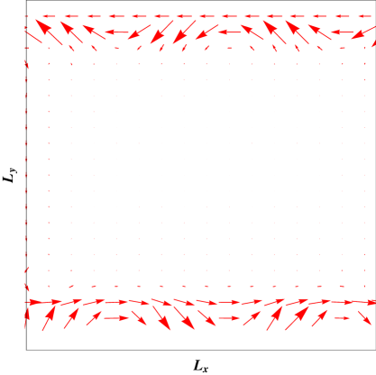
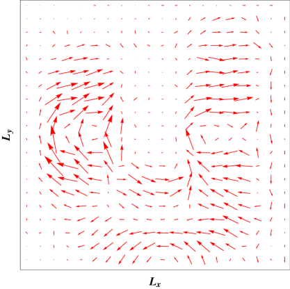
Figure 3: (Color online). Flow of charge current in a perfect ($W=0$) square lattice of size $20\times 20$ considering $B=0.1$, where the left and right panels correspond to $E_{F}=-2.8$ and $-1.46$, respectively. Left panel: Charge current flows only through the edges and no current is obtained in the bulk. Right panel: Charge current flows through the bulk.

zero leading to near complete suppression of the backscattering processes and thereby the momentum relaxation process. In the continuum model these states are referred as the positive and negative $k$-states and they are commonly named as the edge states. At high magnetic field we get practically zero overlap between these states. Due to this complete elimination of momentum relaxation, the edge states carrying current towards the right side of the sample are in equilibrium with the left lead, while the other states carrying current in the opposite direction are in equilibrium with the right lead. Therefore, the difference in voltage measured by two voltage probes placed anywhere on the same side (the so-called longitudinal voltage) of the conductor gets zero, while a non-zero value of the Hall voltage is obtained when it is measured by two voltage probes placed anywhere on the opposite sides of the conductor.

The almost entire suppression of the momentum relaxation process, when Fermi energy lies in the plateau regions, gives rise to essentially zero longitudinal resistance exactly what we have obtained numerically (see the right panel of Fig. 2). The resistance of a conductor is governed by the rate at which the electrons can loose their momentum. To relax the momentum an electron has to be scattered from the left side to the right side of the conductor through the allowed energy eigenstates in the bulk of the conductor. This is practically zero (see the left panel of Fig. 3) as long as the Fermi energy lies between two Landau levels. The non-zero value of the longitudinal resistance is obtained exclusively when the backscattering process takes place and it would be maximum when the Fermi energy synchronizes with a Landau band (right panel of Fig. 2). To articulate the authenticity, in the right panel of Fig. 3, we expose the nature of bond charge current in the conductor when the Fermi energy is fixed at a Landau band ($E_{F}=-1.46$).

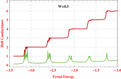
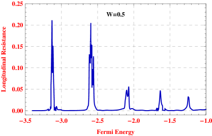
Figure 4: (Color online). Left panel: Hall conductance (red line) as a function of Fermi energy and the electronic density of states (green line) for a disordered ($W=0.5$) square lattice of size $20\times 20$ considering $B=0.05$. Right panel: Longitudinal resistance as a function of Fermi energy for the same parameter values.

It predicts a continuous flow of charge form one edge to the other, and certainly, electrons can scatter from the left to the right side of the conductor through its bulk. This scattering leads to the longitudinal resistance. Thus, each time the Fermi energy crosses a Landau band, we get maximum backscattering and hence a peak in the longitudinal resistance (see the right panel of Fig. 2).

We now present the results for a disordered square lattice of size $20\times 20$ in Fig. 4. Disorder is introduced via a random distribution (width $W=0.5$) of values of the on-site potentials (diagonal disorder), and results averaged over hundred disorder configurations are presented. In the presence of disorder sharp Landau levels are broadened (green line in the left panel of Fig. 4), but it does not affect the quantized nature of the Hall conductance. However, in contrast to the perfect conductor, the sharpness of the Hall conductance gets reduced as observed in the left panel of Fig. 4 (red curve). At the plateau regions the Hall conductance is again precisely quantized in units of $2e^{2}/h$ and such conductance quantization, even in the presence of impurities, comes due to the complete spatial separation of the forward and backward propagating states which becomes apparent in Fig. 5 (left panel). On the other hand, when the Fermi energy lies on a bulk Landau band, electrons can easily scatter through the interior of the conductor, giving rise to non-zero bond charge currents throughout the conductor (right panel of Fig. 5). This scattering yields the longitudinal resistance (see the right panel of Fig. 4).

It is important to note that with the increase of the disorder strength Landau bands get broadened more by virtue of disorder. As a result of disorder localized states are appeared in the tails of the broadened Landau bands and they do not contribute to the transport. But, as we get the non-vanishing Hall conductance, all the states within the Landau bands cannot be localized. At the band centers extended states exist which carry the Hall current and the amount of current which is lost due to the formation of localized states in the tail of a Landau band is exactly compensated by the remaining extended states prange ; ando . Since the localized states within the Landau band do not contribute to the current the Hall plateaus become broadened which has been clearly explained by Kramer et al. kramer . It

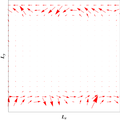
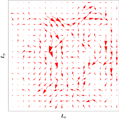
Figure 5: (Color online). Flow of charge current in a disordered ($W=1$) square lattice of size $20\times 20$ considering $B=0.1$, where the left and right panels correspond to $E_{F}=-2.8$ and $-1.46$, respectively. Left panel: Charge current flows only through the edges and no current is obtained in the bulk. Right panel: Charge current flows through the bulk.

is also to be noted that for large enough disorder strength and for weak magnetic field, quantum Hall plateaus gradually vanish from the higher energy side. We confirm it numerically. However, it was not the main motivation of our present work, and the disappearance of the integer quantum Hall effect due to disorder has already been reported in the literature sheng1 ; sheng2 .

Before we end this section, we would like to point out that the disappearance of edge states and the appearance of finite resistance associated with the backscattering processes, as a result of movement of the Fermi level $E_{F}$, strongly depend on the system size, magnetic field and also on the impurity strength. Here we describe very briefly about the nature of quantum phase transition associated with the above mentioned factors, to make the present communication a self contained study. The near zero value of the longitudinal resistance is obtained only when the Fermi energy lies anywhere within the plateau regions and in this situation the backscattering processes are almost suppressed which result edge currents in the sample. While, for all other choices of $E_{F}$, the finite value of longitudinal resistance is obtained i.e., the backscattering processes are dominated which provide bulk current. For a finite system size and fixed disorder strength, the appearance of distinct Landau levels, and hence the quantized nature of Hall plateaus, depends on the choice of the magnetic field. If the field is too weak, then the Hall plateaus will no longer appear and the backscattering processes are also strong enough to produce bulk current. On the other hand, if we fix the system size and choose the magnetic field to a moderate one then the appearance of the edge currents or bulk current upon the movement of the Fermi level is significantly controlled by the impurity strength. For our system size ($20\times 20$) we examine that when $W>2$, the Hall plateaus almost disappear and we get bulk current for any choice of $E_{F}$ and this feature would be visible for much less value of $W$ in the thermodynamic limit. Thus, we can emphasize that the quantum phase transition in the phenomenon of integer quantum Hall effect in a square lattice geometry strongly depends on the system size, disorder strength and the applied magnetic field. For a particular disorder strength and in presence of a moderate magnetic field, a functional dependence of the Fermi energy $E_{F}$ with system size may be obtained for the crossover between the edge currents and bulk currents. Since at this stage it is really too complicated to compute it numerically we can try to establish this functional form in our future work, but, we believe, the main essence of all these features are quite well understood from our present study.

IV Conclusion

In conclusion, we have investigated the phenomenon of integer quantum Hall effect in a discrete lattice model through Landauer-Büttiker formalism. The almost complete suppression of momentum relaxation processes and the oscillating nature of longitudinal resistance are clearly explored by examining the flow of charge current using Landauer-Keldysh prescription. The results presented in this communication are worked out for absolute zero temperature. However, they should remain valid even in a certain range of finite temperatures ($\sim 300$ K). This is because the broadening of the energy levels of the conductor due to the conductor-lead coupling is, in general, much larger than that of the thermal broadening datta . Our present study about QHE based on the discrete lattice model provides much better insight to the problem under realistic condition.

References

- (1) K. von Klitzing, G. Dorda, and M. Pepper, Phys. Rev. Lett. 45, 494 (1980).
- (2) A. Hartland, Metrologia 29, 175 (1992).
- (3) S. Datta, Electronic transport in mesoscopic systems, Cambridge University Press, Cambridge (1995).
- (4) B. I. Halperin, Phys. Rev. B 25, 2185 (1982).
- (5) A. H. MacDonald and P. Streda, Phys. Rev. B 29, 1616 (1984).
- (6) R. B. Laughlin, Phys. Rev. B 23, 5632 (1981).
- (7) D. J. Thouless, M. Kohmoto, M. P. Nightingale, and M. den Nijs, Phys. Rev. Lett. 49, 405 (1982).
- (8) Q. Niu, D. J. Thouless, and Y.-S. Wu, Phys. Rev. B 31, 3372 (1985).
- (9) R. E. Prange, Phys. Rev. B 23, 4802 (1981).
- (10) J. E. Avron and R. Seiler, Phys. Rev. Lett. 54, 259 (1985).
- (11) K. von Klitzing, Rev. Mod. Phys. 58, 519 (1986).
- (12) B. K. Nikolíc, L. P. Zârbo, and S. Souma, Phys. Rev. B 73, 075303 (2006).
- (13) L. P. Zârbo and B. K. Nikolíc, Europhys. Lett. 80, 47001 (2007).
- (14) K. S. Novoselov, A. K. Geim, S. V. Morozov, D. Jiang, M. I. Katsnelson, I. V. Grigorieva, S. V. Dubonos, and A. A. Firsov, Nature (London) 438, 197 (2005).
- (15) Y. Zhang, Y. -W. Tan, H. L. Stormer, and P. Kim, Nature (London) 438, 201 (2005).
- (16) H. Hatami, N. Abedpour, A. Qaiumzadeh, and R. Asgari, Phys. Rev. B 83, 125433 (2011).
- (17) W. Long, Q. -F. Sun, and J. Wang, Phys. Rev. Lett. 101, 166806 (2008).
- (18) M. Janssen, O. Viehweger, U. Fastenrath, and J. Hajdu, Introduction to the theory of the integer quantum Hall effect, Ed. by J. Hajdu, VCH (Federal Republic of Germany) (1994).
- (19) R. E. Prange, Phys. Rev. B 23, 4802 (1981).
- (20) H. Aoki and T. Ando, Solid State Commun. 18, 1079 (1981).
- (21) B. Kramer, S. Kettemann, and T. Ohtsuki, Physica E 20, 172 (2003).
- (22) D. N. Sheng and Z. Y. Weng, Phys. Rev. Lett. 78, 318 (1997).
- (23) D. N. Sheng, Z. Y. Weng, and Q. Gao, Chinese J. Phys. 36, 433 (1988).