Primordial non-Gaussianities of gravitational waves in the most general single-field inflation model

Abstract

We completely clarify the feature of primordial non-Gaussianities of tensor perturbations in generalized G-inflation, i.e., the most general single-field inflation model with second order field equations. It is shown that the most general cubic action for the tensor perturbation (gravitational wave) $h_{ij}$ is composed only of two contributions, one with two spacial derivatives and the other with one time derivative on each $h_{ij}$. The former is essentially identical to the cubic term that appears in Einstein gravity and predicts a squeezed shape, while the latter newly appears in the presence of the kinetic coupling to the Einstein tensor and predicts an equilateral shape. Thus, only two shapes appear in the graviton bispectrum of the most general single-field inflation model, which could open a new clue to the identification of inflationary gravitational waves in observations of cosmic microwave background anisotropies as well as direct gravitational wave detection experiments.

Inflation, an accelerated expansion of the early Universe caused by a scalar field called inflaton, is a quite promising paradigm of cosmology, and primordial perturbations generated from inflation are crucial clues to the yet unidentified inflationary model. From the properties of the primordial perturbations such as the power spectra and spectral indices, we can extract information about the theory governing the inflaton dynamics. Among them the non-Gaussian signature in the cosmic microwave background (CMB) has been paid much attention in recent years, along with the great progress in precise cosmological observations. So far most of the literature has focused upon non-Gaussianities of the scalar perturbations malda1 , as they are most directly connected to the CMB observations. Tensor perturbations Sta , however, are also generated during inflation, whose direct detection would be the most obvious evidence for inflation. When we try to detect tensor perturbations with the CMB measurements and/or with the direct detection experiments, it is essentially important to remove the background (contamination) sources. For example, the B-mode polarizations are dominated by the lensing effects on relatively small scales. Astrophysical sources like white dwarf binaries could dominate the power spectrum for a wide range of frequencies of the background gravitational waves. Thus, non-Gaussianities will be a key feature of the tensor perturbations malda2 ; soda as well as the scalar perturbations because they can help us to discriminate the inflationary signals from other contamination sources even if the latter dominates the power spectrum. For this purpose, we need to completely clarify the features of the non-Gaussianities of primordial tensor perturbations produced during inflation, which enables us to make templates for non-Gaussianities of primordial gravitational waves.

In this Letter, we, for the first time, investigate the non-Gaussianities of primordial tensor perturbations based on the most general single-field inflation model, i.e., generalized G-inflation G2 , make a complete identification of the shapes of bispectra, and explore the possibility of large non-Gaussianities from the tensor sector.

The Lagrangian for generalized G-inflation is the most general one that is composed of the metric $g_{\mu\nu}$, the scalar field $\phi$, and their arbitrary derivatives, and has the second-order field equations. The Lagrangian was first derived by Horndeski in 1974 Horndeski , and very recently it was rediscovered in a modern form as the generalized Galileon GG , i.e., the most general extension of the Galileon Galileon ; CovGali , in four dimensions. The generalized Galileon is described by the sum of the following four:

$${\cal L}_{2}=K(\phi,X),\quad{\cal L}_{3}=-G_{3}(\phi,X)\Box\phi,$$ (1)

$${\cal L}_{4}=G_{4}(\phi,X)R+G_{4X}\left[(\Box\phi)^{2}-(\nabla_{\mu}\nabla_{\nu}\phi)^{2}\right],$$ (2)

$${\cal L}_{5}=G_{5}(\phi,X)G_{\mu\nu}\nabla^{\mu}\nabla^{\nu}\phi-\frac{1}{6}G_{5X}\bigl{[}(\Box\phi)^{3}$$ (3)

$$\qquad\qquad\qquad-3\Box\phi(\nabla_{\mu}\nabla_{\nu}\phi)^{2}+2(\nabla_{\mu}\nabla_{\nu}\phi)^{3}\bigr{]},$$ (4)

where $K$ and $G_{i}$’s are arbitrary functions of $\phi$ and $X:=-(\partial\phi)^{2}/2$. Here we used the notation $G_{iX}$ for $\partial G_{i}/\partial X$. The generalized Galileon can be used as a framework to study the most general single-field inflation model. Generalized G-inflation contains novel models, as well as previously known models of single-field inflation such as standard canonical inflation, k-inflation kinf , extended inflation extinf , $R^{2}$ inflation R2inf , new Higgs inflation newhiggs , and (minimal) G-inflation Ginf . The above four Lagrangians can even reproduce the non-minimal coupling to the Gauss-Bonnet term G2 .

In G2 , the background equations for generalized G-inflation is presented, and the most general quadratic actions for tensor and scalar perturbations are determined, giving the power spectra of the primordial perturbations. The most general cubic action for scalar perturbations is worked out in Gao ; Tsujikawa . The curvature perturbation in generalized G-inflation is shown to be conserved on large scales at non-linear order in Gao2 . We are going to present the most general cubic action for tensor perturbations to determine the possible tensor bispectrum arising from single-field inflation.

The perturbed metric around a cosmological background may be written as

$$g_{00}=-1,\quad g_{0i}=0,\quad g_{ij}=a^{2}(t)\left(e^{h}\right)_{ij},$$ (5)

where

$$\left(e^{h}\right)_{ij}=\delta_{ij}+h_{ij}+\frac{1}{2}h_{ik}h_{kj}+\frac{1}{6}h_{ik}h_{kl}h_{lj}+\cdots,$$ (6)

and $h_{ij}$ is a transverse and traceless tensor perturbation, $\partial_{i}h_{ij}=0=h_{ii}$, with repeated spatial indices summarized by $\delta_{ij}$. The perturbed metric defined in this way is convenient for calculating the action because we have $\sqrt{-g}=a^{3}$. We plug the metric (5) into the action

$$S=\sum_{i=2}^{5}\int{\rm d}^{4}x\sqrt{-g}{\cal L}_{i},$$ (7)

and expand it in terms of $h_{ij}$ to get the quadratic and cubic actions. Only the Lagrangians that involve the curvature tensors and $\nabla_{\mu}\nabla_{\nu}\phi$, i.e., ${\cal L}_{4}$ and ${\cal L}_{5}$, contribute to the quadratic and cubic actions.

The quadratic action was already derived in G2 :

$$S^{(2)}=\frac{1}{8}\int{\rm d}t{\rm d}^{3}x\,a^{3}\left[{\cal G}_{T}\dot{h}_{ij}^{2}-\frac{{\cal F}_{T}}{a^{2}}(\partial_{k}h_{ij})^{2}\right],$$ (8)

where an overdot denotes ${\rm d}/{\rm d}t$ and

$${\cal F}_{T} := 2\left[G_{4}-X\left(\ddot{\phi}G_{5X}+G_{5\phi}\right)\right],$$ (9)

$${\cal G}_{T} := 2\left[G_{4}-2XG_{4X}-X\left(H\dot{\phi}G_{5X}-G_{5\phi}\right)\right].\;\;$$ (10)

From the action we see that the propagation speed of the gravitational waves is given by $c_{h}:=\sqrt{{\cal F}_{T}/{\cal G}_{T}}$, which may differ from unity. In order for the system to be stable ${\cal F}_{T}>0$ and ${\cal G}_{T}>0$ are required.

The linear perturbation equation derived from the action (8) can be solved in the Fourier space,

$$h_{ij}(t,\mathbf{x})=\int\frac{{\rm d}^{3}k}{(2\pi)^{3}}\,\tilde{h}_{ij}(t,\mathbf{k})e^{i\mathbf{k}\cdot\mathbf{x}}.$$ (11)

To proceed further, it is convenient to introduce a new time coordinate defined by ${\rm d}y=c_{h}{\rm d}t/a$. We assume for simplicity that the inflationary Universe may be approximated by de Sitter spacetime and ${\cal F}_{T}$ and ${\cal G}_{T}$ are approximately constant. Using the normalized mode solution,

$$\psi_{\mathbf{k}}=\frac{\sqrt{\pi}}{a}\sqrt{\frac{c_{h}}{{\cal F}_{T}}}\sqrt{-y}H_{3/2}^{(1)}(-ky),$$ (12)

where $H^{(1)}_{3/2}$ is the Hankel function, the quantized tensor perturbation is written as

$$\tilde{h}_{ij}=\sum_{s}\left[\psi_{\mathbf{k}}e_{ij}^{(s)}(\mathbf{k})a_{s}(\mathbf{k})+\psi^{*}_{-\mathbf{k}}e_{ij}^{*(s)}(-\mathbf{k})a_{s}^{\dagger}(-\mathbf{k})\right],$$ (13)

where $e_{ij}^{(s)}$ is the polarization tensor with the helicity states $s=\pm 2$, satisfying $e_{ii}^{(s)}(\mathbf{k})=0=k_{j}e_{ij}^{(s)}(\mathbf{k})$. Here we adopt the normalization such that $e_{ij}^{(s)}(\mathbf{k})e_{ij}^{*(s^{\prime})}(\mathbf{k})=\delta_{ss^{\prime}}$. Choosing the phase of the polarization tensors appropriately, we have the relations $e_{ij}^{*(s)}(\mathbf{k})=e_{ij}^{(-s)}(\mathbf{k})=e_{ij}^{(s)}(-\mathbf{k})$. The commutation relation for the creation and annihilation operators is given by $[a_{s}(\mathbf{k}),a_{s^{\prime}}^{\dagger}(\mathbf{k}^{\prime})]=(2\pi)^{3}\delta_{ss^{\prime}}\delta(\mathbf{k}-\mathbf{k^{\prime}})$. The 2-point function can now be computed as

$$\langle\tilde{h}_{ij}(\mathbf{k})\tilde{h}_{kl}(\mathbf{k}^{\prime})\rangle = (2\pi)^{3}\delta^{(3)}(\mathbf{k}+\mathbf{k}^{\prime}){\cal P}_{ij,kl}(\mathbf{k}),$$ (14)

$${\cal P}_{ij,kl} = |\psi_{\mathbf{k}}|^{2}\Pi_{ij,kl}(\mathbf{k}),$$ (15)

where we introduced

$$\Pi_{ij,kl}(\mathbf{k})=\sum_{s}e_{ij}^{(s)}(\mathbf{k})e_{kl}^{*(s)}(\mathbf{k}).$$ (16)

The power spectrum ${\cal P}_{h}=(k^{3}/2\pi^{2}){\cal P}_{ij,ij}$ is given by

$${\cal P}_{h}(k)=\left.\frac{1}{2\pi^{2}}\frac{H^{2}}{{\cal F}_{T}c_{h}}\right|_{ky=-1},$$ (17)

where $y=-1/k$ corresponds to the time of the sound horizon exit.

Having thus obtained the quadratic action and the solution to the linearized equation governing the inflationary gravitational waves, we now move on to the cubic action. The most general cubic action for tensor perturbations in the single-field context is obtained as

$$S^{(3)} = \int{\rm d}t{\rm d}^{3}x\,a^{3}\biggl{[}\frac{X\dot{\phi}G_{5X}}{12}\dot{h}_{ij}\dot{h}_{jk}\dot{h}_{ki}$$ (18)

$$\qquad+\frac{{\cal F}_{T}}{4a^{2}}\left(h_{ik}h_{jl}-\frac{1}{2}h_{ij}h_{kl}\right)\partial_{k}\partial_{l}h_{ij}\biggr{]},$$

which is composed only of two contributions. Clearly, the term with one time derivative on each $h_{ij}$ appears only if $G_{5X}\neq 0$. This term is absent in the case of Einstein gravity, non-minimal coupling to gravity (${\cal L}_{3}=f(\phi)R$), and even in the case of new Higgs inflation which involves a non-standard kinetic term of the form $G^{\mu\nu}\partial_{\mu}\phi\partial_{\nu}\phi$ . However, in the presence of non-minimal coupling to the Gauss-Bonnet term, this term does not vanish G2 . The terms of the form $h^{2}\partial^{2}h$, where $\partial$ represents a spatial derivative, is already present in the case of Einstein gravity, and even in the most general case only the overall normalization is generalized from the Planck mass squared $M_{\rm Pl}^{2}$ to the function ${\cal F}_{T}$.

The 3-point function can be computed by employing the in-in formalism,

$$\langle\tilde{h}_{i_{1}j_{1}}(\mathbf{k}_{1})\tilde{h}_{i_{2}j_{2}}(\mathbf{k}_{2})\tilde{h}_{i_{3}j_{3}}(\mathbf{k}_{3})\rangle$$

$$=-i\int^{t}_{t_{0}}{\rm d}t^{\prime}\langle[\tilde{h}_{i_{1}j_{1}}(t,\mathbf{k}_{1})\tilde{h}_{i_{2}j_{2}}(t,\mathbf{k}_{2})\tilde{h}_{i_{3}j_{3}}(t,\mathbf{k}_{3}),H_{\rm int}(t^{\prime})]\rangle,$$

where $t_{0}$ is some early time when the perturbation is well inside the sound horizon, $t$ is a time several e-foldings after the sound horizon exit, and the interaction Hamiltonian is

$$H_{\rm int}(t)=-\int{\rm d}^{3}x\,a^{3}\biggl{[}\frac{X\dot{\phi}G_{5X}}{12}\dot{h}_{ij}\dot{h}_{jk}\dot{h}_{ki}+\cdots\biggr{]}.$$ (19)

It will be convenient to introduce the non-Gaussian amplitude ${\cal A}_{i_{1}j_{1}i_{2}j_{2}i_{3}j_{3}}$ defined by

$$\langle\tilde{h}_{i_{1}j_{1}}(\mathbf{k}_{1})\tilde{h}_{i_{2}j_{2}}(\mathbf{k}_{2})\tilde{h}_{i_{3}j_{3}}(\mathbf{k}_{3})\rangle$$

$$\quad=(2\pi)^{7}\delta^{(3)}(\mathbf{k}_{1}+\mathbf{k}_{2}+\mathbf{k}_{3}){\cal P}_{h}^{2}\frac{{\cal A}_{i_{1}j_{1}i_{2}j_{2}i_{3}j_{3}}}{k_{1}^{3}k_{2}^{3}k_{3}^{3}}.$$ (20)

We write ${\cal A}_{i_{1}j_{1}i_{2}j_{2}i_{3}j_{3}}={\cal A}^{({\rm new})}_{i_{1}j_{1}i_{2}j_{2}i_{3}j_{3}}+{\cal A}^{({\rm GR})}_{i_{1}j_{1}i_{2}j_{2}i_{3}j_{3}}$, where ${\cal A}^{({\rm new})}_{i_{1}j_{1}i_{2}j_{2}i_{3}j_{3}}$ and ${\cal A}^{({\rm GR})}_{i_{1}j_{1}i_{2}j_{2}i_{3}j_{3}}$ represent the contributions from the $\dot{h}^{3}$ term and the $h^{2}\partial^{2}h$ terms, respectively. Just for simplicity, here again the inflationary Universe is approximated by de Sitter spacetime, which allows us to to compute the non-Gaussian amplitude assuming that $X\dot{\phi}G_{5X}\simeq$ const and ${\cal F}_{T}\simeq$ const. Each contribution is then found to be

$${\cal A}_{i_{1}j_{1}i_{2}j_{2}i_{3}j_{3}}^{({\rm new})} = \frac{HX\dot{\phi}G_{5X}}{4{\cal G}_{T}}\frac{k_{1}^{2}k_{2}^{2}k_{3}^{2}}{K^{3}}\Pi_{i_{1}j_{1},lm}(\mathbf{k}_{1})\Pi_{i_{2}j_{2},mn}(\mathbf{k}_{2})\Pi_{i_{3}j_{3},nl}(\mathbf{k}_{3}),$$ (21)

$${\cal A}_{i_{1}j_{1}i_{2}j_{2}i_{3}j_{3}}^{({\rm GR})} = \tilde{\cal A}\left\{\Pi_{i_{1}j_{1},ik}(\mathbf{k}_{1})\Pi_{i_{2}j_{2},jl}(\mathbf{k}_{2})\left[k_{3k}k_{3l}\Pi_{i_{3}j_{3},ij}(\mathbf{k}_{3})-\frac{1}{2}k_{3i}k_{3k}\Pi_{i_{3}j_{3},jl}(\mathbf{k}_{3})\right]+5~{}{\rm perms}~{}{\rm of}~{}1,2,3\right\},\;\;\;$$ (22)

where $K=k_{1}+k_{2}+k_{3}$ and

$$\tilde{\cal A}(k_{1},k_{2},k_{3}):=-\frac{K}{16}\biggl{[}1-\frac{1}{K^{3}}\sum_{i\neq j}k_{i}^{2}k_{j}-4\frac{k_{1}k_{2}k_{3}}{K^{3}}\biggr{]}.\;\;\;$$ (23)

We see that the second contribution, which is present in the case of Einstein gravity, is independent of any functions in the Lagrangian, and hence for all the models of single-field inflation ${\cal A}_{i_{1}j_{1}i_{2}j_{2}i_{3}j_{3}}^{({\rm GR})}$ coincides with the one in general relativity. (For this reason we associate this piece of the amplitude with the superscript “GR.”) The size of the first contribution, ${\cal A}_{i_{1}j_{1}i_{2}j_{2}i_{3}j_{3}}^{({\rm new})}$, is crucially dependent on how $\phi$ couples to gravity along the inflationary trajectory. Only those two amplitudes are sufficient to characterize the tensor bispectrum in the most general single-field inflation model.

We are now in position to discuss whether or not large non-Gaussianities can be obtained from ${\cal A}_{i_{1}j_{1}i_{2}j_{2}i_{3}j_{3}}^{({\rm new})}$. Since ${\cal G}_{T}\supset HX\dot{\phi}G_{5X}$, the ratio $HX\dot{\phi}G_{5X}/{\cal G}_{T}$ cannot be large in models with large $HX\dot{\phi}G_{5X}$. The only possibility is that various terms in ${\cal G}_{T}$ are arranged to cancel each other to give ${\cal G}_{T}\sim 0$. (Note, however, that ${\cal G}_{T}$ must be finite and positive.) This then yields ${\cal F}_{S}\sim-{\cal F}_{T}$, where ${\cal F}_{S}$ is the coefficient of $(\partial\zeta)^{2}$ in the quadratic action of the curvature perturbation $\zeta$ and must be positive to avoid gradient instabilities (see Ref. G2 ). Therefore, models with small ${\cal G}_{T}$ tend to be unstable against either scalar or tensor perturbations. For this reason, generally speaking, it is rather non-trivial to get large non-Gaussianities from the $\dot{h}^{3}$ term, though one cannot completely deny the possibility of making both ${\cal F}_{S}$ and ${\cal F}_{T}$ positive with the help of the functional degrees of freedom of our Lagrangian.

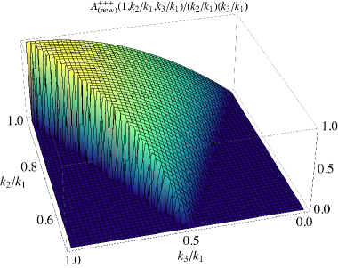
Figure 1: ${\cal A}_{({\rm new})}^{+++}(1,k_{2}/k_{1},k_{3}/k_{1})(k_{2}/k_{1})^{-1}(k_{3}/k_{1})^{-1}$ as a function of $k_{2}/k_{1}$ and $k_{3}/k_{1}$. The plot is normalized to unity for equilateral configurations $k_{2}/k_{1}=k_{3}/k_{1}=1$.

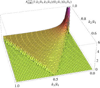
Figure 2: ${\cal A}_{({\rm GR})}^{+++}(1,k_{2}/k_{1},k_{3}/k_{1})(k_{2}/k_{1})^{-1}(k_{3}/k_{1})^{-1}$ as a function of $k_{2}/k_{1}$ and $k_{3}/k_{1}$. The plot is normalized to unity for equilateral configurations $k_{2}/k_{1}=k_{3}/k_{1}=1$.

Let us turn to the two polarization modes,

$$\xi^{(s)}(\mathbf{k}):=\tilde{h}_{ij}(\mathbf{k})e^{*(s)}_{ij}(\mathbf{k}),$$ (24)

and consider their amplitudes ${\cal A}^{s_{1}s_{2}s_{3}}$ of the bispectra $\langle\xi^{s_{1}}(\mathbf{k}_{1})\xi^{s_{2}}(\mathbf{k}_{2})\xi^{s_{3}}(\mathbf{k}_{3})\rangle$. The amplitude may be defined in an analogous way to Eq. (20), so that ${\cal A}_{({\rm new}),({\rm GR})}^{s_{1}s_{2}s_{3}}=e_{i_{1}j_{1}}^{*(s_{1})}(\mathbf{k}_{1})e_{i_{2}j_{2}}^{*(s_{2})}(\mathbf{k}_{2})e_{i_{3}j_{3}}^{*(s_{3})}(\mathbf{k}_{3}){\cal A}_{i_{1}j_{1}i_{2}j_{2}i_{3}j_{3}}^{({\rm new}),({\rm GR})}$. We thus obtain

$${\cal A}_{({\rm new})}^{s_{1}s_{2}s_{3}} = \frac{HX\dot{\phi}G_{5X}}{4{\cal G}_{T}}\frac{k_{1}^{2}k_{2}^{2}k_{3}^{2}}{K^{3}}F_{({\rm new})}^{s_{1}s_{2}s_{3}}(k_{1},k_{2},k_{3}),$$ (25)

$${\cal A}_{({\rm GR})}^{s_{1}s_{2}s_{3}} = \tilde{\cal A}(k_{1},k_{2},k_{3})F_{({\rm GR})}^{s_{1}s_{2}s_{3}}(k_{1},k_{2},k_{3}),$$ (26)

where we defined

$$F_{({\rm new})}^{+++}(k_{1},k_{2},k_{3}):=\frac{K^{3}}{64k_{1}^{2}k_{2}^{2}k_{3}^{2}}$$

$$\qquad\qquad\qquad\qquad\times\biggl{[}K^{3}-4\sum_{i\neq j}k_{i}^{2}k_{j}-4k_{1}k_{2}k_{3}\biggr{]},\;\;\;\;\;\;\;\;$$ (27)

$F_{({\rm GR})}^{+++}(k_{1},k_{2},k_{3}):=K^{2}F_{({\rm new})}^{+++}(k_{1},k_{2},k_{3})/2$, and $F_{({\rm new}),({\rm GR})}^{++-}(k_{1},k_{2},k_{3}):=F_{({\rm new}),({\rm GR})}^{+++}(k_{1},k_{2},-k_{3})$. Since our theory accommodates no parity violation, we have $F^{---}_{({\rm new}),({\rm GR})}=F^{+++}_{({\rm new}),({\rm GR})}$ and $F^{--+}_{({\rm new}),({\rm GR})}=F^{++-}_{({\rm new}),({\rm GR})}$.

The non-Gaussian amplitudes ${\cal A}_{({\rm new})}^{+++}$ and ${\cal A}_{({\rm GR})}^{+++}$ are plotted in Figs. 1 and 2. One sees that the amplitude of the new contribution peaks in the equilateral configuration, while the “GR” contribution becomes largest in the squeezed limit. This gives a clear distinction between the two different contributions, and the two characteristic shapes would be helpful to discriminate the inflationary gravitational waves from those produced by other sources. The other correlation functions such as the $-++$ one are subdominant relative to the $+++$ one because for equilateral configurations $F_{({\rm new})}^{++-}=F_{({\rm new})}^{+-+}=F_{({\rm new})}^{-++}=F_{({\rm new})}^{+++}/9$ and $F_{({\rm GR})}^{++-}=F_{({\rm GR})}^{+-+}=F_{({\rm GR})}^{-++}=F_{({\rm GR})}^{+++}/81$, and in the squeezed limit, $\mathbf{k}_{3}\to 0$, one has $F_{({\rm GR})}^{+++}\approx F_{({\rm GR})}^{++-}\approx-k_{1}^{2}/2$ and $F_{({\rm GR})}^{+-+}\approx F_{({\rm GR})}^{-++}\approx-k_{3}^{4}/32k_{1}^{2}$.

In this Letter, we have clarified primordial non-Gaussianities of tensor perturbations arising from the most general single-field inflation model with second-order field equations, and have found that they are completely determined by two different contributions: ${\cal A}_{({\rm new})}$ and ${\cal A}_{({\rm GR})}$. Our results provide at least two distinctive features to test the framework of generalized G-inflation based on the graviton non-Gaussianities. Firstly, ${\cal A}_{({\rm new})}$ is a unique feature of the kinetic coupling term $G_{5}$. Any detection of this type of bispectrum, no matter large or small, would unambiguously indicate the existence of non-vanishing $G_{5X}$, at least in the Galileon framework. Secondly, the contribution ${\cal A}_{({\rm GR})}$ is a fixed and universal feature for single-field inflation models which are all within the generalized G-inflation framework. It is impossible to enhance/suppress this contribution in generalized G-inflation models. In other words, any detection of enhancement/suppression of this contribution to the graviton bispectrum would imply new physics beyond generalized G-inflation and/or other astrophysical sources. The two contributions are clearly distinguishable according to their shapes of non-Gaussianities.

References

(1)
J. M. Maldacena,
JHEP 0305, 013 (2003).
[astro-ph/0210603].
(2)
A. A. Starobinsky,
JETP Lett. 30, 682 (1979)
[Pisma Zh. Eksp. Teor. Fiz. 30, 719 (1979)].
(3)
J. M. Maldacena, G. L. Pimentel,
[arXiv:1104.2846 [hep-th]].
(4)
J. Soda, H. Kodama, M. Nozawa,
[arXiv:1106.3228 [hep-th]].
(5)
T. Kobayashi, M. Yamaguchi, J. Yokoyama,
[arXiv:1105.5723 [hep-th]].
(6)
G. W. Horndeski, Int. J. Theor. Phys. 10 (1974) 363-384.
(7)
C. Deffayet, X. Gao, D. A. Steer, G. Zahariade,
[arXiv:1103.3260 [hep-th]].
(8)
A. Nicolis, R. Rattazzi, E. Trincherini,
Phys. Rev. D79, 064036 (2009).
[arXiv:0811.2197 [hep-th]].
(9)
C. Deffayet, G. Esposito-Farese, A. Vikman,
Phys. Rev. D79, 084003 (2009).
[arXiv:0901.1314 [hep-th]].
(10)
C. Armendariz-Picon, T. Damour, V. F. Mukhanov,
Phys. Lett. B458, 209-218 (1999).
[hep-th/9904075].
(11)
D. La and P. J. Steinhardt,
Phys. Rev. Lett. 62, 376 (1989)
[Erratum-ibid. 62, 1066 (1989)].
(12)
A. A. Starobinsky,
Phys. Lett. B 91, 99 (1980).
(13)
C. Germani, A. Kehagias,
Phys. Rev. Lett. 105, 011302 (2010).
[arXiv:1003.2635 [hep-ph]].
(14)
T. Kobayashi, M. Yamaguchi, J. Yokoyama,
Phys. Rev. Lett. 105, 231302 (2010).
[arXiv:1008.0603 [hep-th]];
K. Kamada, T. Kobayashi, M. Yamaguchi, J. Yokoyama,
Phys. Rev. D83, 083515 (2011).
[arXiv:1012.4238 [astro-ph.CO]];
T. Kobayashi, M. Yamaguchi, J. ’i. Yokoyama,
Phys. Rev. D83, 103524 (2011).
[arXiv:1103.1740 [hep-th]];
C. Deffayet, O. Pujolas, I. Sawicki, A. Vikman,
JCAP 1010, 026 (2010).
[arXiv:1008.0048 [hep-th]].
(15)
X. Gao, D. A. Steer,
[arXiv:1107.2642 [astro-ph.CO]].
(16)
A. De Felice, S. Tsujikawa,
[arXiv:1107.3917 [gr-qc]].