Buckling of Spherical Capsules

Abstract

We investigate buckling of soft elastic capsules under negative pressure or for reduced capsule volume. Based on nonlinear shell theory and the assumption of a hyperelastic capsule membrane, shape equations for axisymmetric and initially spherical capsules are derived and solved numerically. A rich bifurcation behavior is found, which is presented in terms of bifurcation diagrams. The energetically preferred stable configuration is deduced from a least-energy principle both for prescribed volume and prescribed pressure. We find that buckled shapes are energetically favorable already at smaller negative pressures and larger critical volumes than predicted by the classical buckling instability. By preventing self-intersection for strongly reduced volume, we obtain a complete picture of the buckling process and can follow the shape from the initial undeformed state through the buckling instability into the fully collapsed state. Interestingly, the sequences of bifurcations and stable capsule shapes differ for prescribed volume and prescribed pressure. In the buckled state, we find a relation between curvatures at the indentation rim and the bending modulus, which can be used to determine elastic moduli from experimental shape analysis.

I Introduction

An elastic capsule consists of an elastic membrane enclosing a fluid phase. Elastic capsules are commonly met in nature, prominent examples are red blood cells or virus capsules. Artificial capsules can be fabricated by various methods Meier2000 , for example by interfacial polymerization at liquid droplets Rehage2002 or by multilayer deposition of polyelectrolytes Donath1998 , and have numerous applications. Sizes of capsules vary from the nanometer to the micrometer regime, and their mechanical properties depend on the fabrication process. For various applications, for example, if capsules are used as delivery and release systems, there is a need to characterize mechanical properties of capsules. The shape of capsules is approximately spherical but capsules are easily deformed by shear flow Barthes-Biesel2011 , rotation Pieper1998 , in adhesion Komura2005 ; Graf2006 , or by the application of local forces Fery2004 ; Fery2007 ; Zoldesi2008 . Their deformation behavior also exhibits buckling instabilities upon decreasing the interior pressure or the enclosed volume Gao2001 ; Fery2004 ; Zoldesi2008 ; Sacanna2011 or in adhesion Komura2005 . All these deformation modes can potentially be used in experiments to infer material properties of capsules.

Changes of the pressure inside the capsule by osmosis or mechanical means and changes in the capsule volume represent the most basic deformation mechanisms for capsules with spherical rest shape. In this article, we study the collapse of a three-dimensional spherical capsule via the buckling instability into a fully collapsed state under negative pressure or for reduced capsule volume. The mechanical buckling instability sets in at the classical buckling pressure, which is well-known within linear shell theory for small displacements and an isotropic material LL7 and has recently been extended to shell materials with anisotropic shear response Ru2009 . The classical buckling pressure $p_{cb}\propto-E(H_{0}/R_{0})^{2}$, where $E$ is Young’s modulus, $H_{0}$ the initial membrane thickness and $R_{0}$ its initial diameter, can be used in experiments to determine Young’s modulus of the capsule material Gao2001 ; Fery2004 .

While the classical buckling pressure only marks the onset of the instability within linear shell theory and, thus, the limits of stability of a spherical capsule, it is much more difficult to calculate buckled shapes beyond the critical buckling pressure because larger deformations require nonlinear theories and contact between originally opposite capsule sides has to be included in order to prevent self-intersections. Some nonlinear theories have been applied to compute axisymmetric shapes with large deformations, for example in Blyth2004 under the assumption of isotropic tensions and for a more general case in Bauer1970 . Large buckling deformations have been considered numerically based on triangulated surface models Komura2005 ; Vliegenthart2011 ; Quilliet2008 ; Marmottant2011 . In the framework of shell theory, however, a complete picture of the transition into buckled shapes as observed in the experiments is still lacking.

In order to develop this picture for axisymmetric capsules, we use a nonlinear shell theory Libai1998 ; Pozrikidis2003 and assume hyperelastic capsule membranes. For hyperelastic materials, a strain-energy function exists from which the tensions and bending moments can be deduced. It can be shown in general that solutions of the equations of force and moment equilibrium render the functional of total energy stationary Libai1998 . This allows us to combine two tools, force equilibrium and principle of minimal energy, in order to find different branches of stationary deformed capsule shapes and then determine which capsule shape among different branches represents the global energy minimum. At the classical buckling instability the branch corresponding to a spherical capsule loses stability and a bifurcation to buckled shapes takes place. This bifurcation is analyzed in detail beyond a linear stability analysis and in energy (and enthalpy) bifurcation diagrams. We find that the buckling transition is discontinuous in the energy diagrams and that the buckled shape becomes energetically favorable already at a smaller negative pressure $|p_{c}|<|p_{cb}|$ than the classical buckling pressure, where the spherical shape becomes mechanically unstable.

We extend our approach to capsules with opposite sides in contact in order to prevent self-intersection at strongly reduced capsule volume. As far as we know, this has so far only been achieved for elastic rings Flaherty1972 in two dimensions, but not for spherical shells in three dimensions.

Furthermore, we analyze features of buckled shapes, in particular, the maximal curvature occurring at the edge of the indentation rim and find a relation between the maximal curvatures and the bending modulus, which can be used in experimental shape analysis.

II Finite Strain Shell Theory

II.1 Geometric Setup

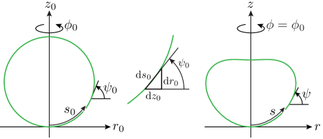
Figure 1: (Color online) Parameterization of the undeformed (left; always with index “0”) and deformed midsurface

We consider axisymmetric capsules, which are undergoing axisymmetric, torsionless deformations and whose membrane thickness is small compared to the other capsule dimensions. The midsurface of the undeformed capsule is parameterized by the curvilinear coordinates $s_{0}\in[0,\,L_{0}]$ and $\phi_{0}\in[0,\,2\pi)$ denoting the arc length measured along the meridian and the angle of revolution, respectively. Its shape is determined by the functions $r_{0}(s_{0})$ and $z_{0}(s_{0})$ in cylindrical polar coordinates (see figure 1).

In addition to the functions $r_{0}(s_{0})$ and $z_{0}(s_{0})$, the slope angle $\psi_{0}(s_{0})$ is defined via the relations (see figure 1)

$$\frac{\mathrm{d}r_{0}}{\mathrm{d}s_{0}}=\cos\psi_{0}\quad\text{and}\quad\frac{\mathrm{d}z_{0}}{\mathrm{d}s_{0}}=\sin\psi_{0}.$$ (1)

Using this parameterization we calculate the principal curvatures of the midsurface,

$$\kappa_{s_{0}}=\frac{\mathrm{d}\psi_{0}}{\mathrm{d}s_{0}}\quad\text{and}\quad\kappa_{\phi_{0}}=\frac{\sin\psi_{0}}{r_{0}}.$$ (2)

Here, $\kappa_{s_{0}}$ denotes the curvature in the meridional direction, and $\kappa_{\phi_{0}}$ the curvature in the circumferential direction.

For the special case of capsules with spherical resting shape, the parameterization of the undeformed midsurface is known analytically,

$$r_{0}(s_{0}) =R_{0}\,\sin\left(s_{0}/R_{0}\right)\quad\text{and}$$ (3)

$$z_{0}(s_{0}) =R_{0}\,\left[1-\cos\left(s_{0}/R_{0}\right)\right],$$

where the arc length $s_{0}$ ranges up to $L_{0}=\pi\,R_{0}$. Accordingly, the slope angle and curvatures are given by

$$\psi_{0}(s_{0})={s_{0}/R_{0}}\quad\text{and}\quad\kappa_{s_{0}}=\kappa_{\phi_{0}}={1}/{R_{0}},$$ (4)

respectively.

All quantities introduced so far in this section carry the index “$0$” because they refer to the undeformed capsule configuration. The midsurface of the deformed configuration is parameterized using analogous quantities without indices “$0$”. Specifically, its shape is determined by the sought-after functions $r(s)$, $z(s)$ and the redundant $\psi(s)$. These functions have to satisfy the boundary conditions $r(0)=r(L)=z(0)=0$, $\psi(0)=0$ and $\psi(L)=\pi$, corresponding to a closed capsule without kinks at its poles. The geometrical relations (1) and (2) can be transferred directly to the deformed midsurface by omitting all indices “$0$”.

II.2 Measures of Deformation

Having defined the parameterization of the deformed and undeformed midsurface, we can now introduce measures of deformation. Fibers oriented along the meridional and circumferential direction get stretched by the factors

$$\lambda_{s}=\frac{\mathrm{d}s}{\mathrm{d}s_{0}}=s^{\prime}(s_{0})\quad\text{and}\quad\lambda_{\phi}=\frac{r}{r_{0}},$$ (5)

respectively. The function $s(s_{0})$ defined in this context describes the position $s$ at which a particle can be found that was originally located at $s_{0}$. In order to center the measures of stretch around zero, we define the meridional and circumferential strains $e_{s}=\lambda_{s}-1$ and $e_{\phi}=\lambda_{\phi}-1$. The bending of the midsurface is measured by the meridional and circumferential bending strains

$$K_{s}=\lambda_{s}\,\kappa_{s}-\kappa_{s_{0}}\quad\text{and}\quad K_{\phi}=\lambda_{\phi}\,\kappa_{\phi}-\kappa_{\phi_{0}}.$$ (6)

They are more suitable than a simple difference of deformed and undeformed curvature because they lead to more simple constitutive equations, as we will see below.

II.3 Elastic Law

The strains measured by $e_{s}$, $e_{\phi}$, $K_{s}$ and $K_{\phi}$ give rise to elastic tensions and bending moments in the capsule membrane. Assuming that the capsule membrane consists of an hyperelastic material, there exists a surface energy density $w_{S}(e_{s},\,e_{\phi},\,K_{s},\,K_{\phi})$, which measures the elastic energy that is stored in an infinitesimal patch of the membrane divided by the area that this patch takes in the undeformed configuration. In this paper, we will use a Hookean model Libai1998

$$w_{S}=\frac{1}{2}\frac{E\,H_{0}}{1-\nu^{2}}\left(e_{s}^{2}+2\,\nu\,e_{s}\,e_{\phi}+e_{\phi}^{2}\right)\\ +\frac{1}{2}E_{B}\left(K_{s}^{2}+2\,\nu\,K_{s}\,K_{\phi}+K_{\phi}^{2}\right)$$ (7)

with a (three-dimensional) Young modulus $E$, a bending modulus $E_{B}$, and a Poisson ratio $\nu$, for a shell of (homogeneous) thickness $H_{0}$. Note that the Poisson ratio of a two-dimensional membrane can take values $-1\leq\nu\leq 1$, with $\nu=1$ corresponding to an area-incompressible membrane. The product $E\,H_{0}$ is frequently called the surface Young modulus. In classical small strain theory of plates, the bending modulus can be expressed as

$$E_{B}=\frac{E\,H_{0}^{3}}{12(1-\nu^{2})}.$$ (8)

The bending energy contribution in the elastic energy (7) agrees to leading order in $e_{s}$ and $e_{\phi}$ (where $K_{s}=\kappa_{s}-\kappa_{s_{0}}$ and $K_{\phi}=\kappa_{\phi}-\kappa_{\phi_{0}}$) and for an incompressible membrane with $\nu=1$ with the commonly used Helfrich bending energy $(\kappa_{s}+\kappa_{\phi}-c_{0})^{2}$ (see e.g. Quilliet2008 ; Marmottant2011 ) with a spontaneous curvature $c_{0}=\kappa_{s_{0}}+\kappa_{\phi_{0}}$. The Helfrich bending energy was originally proposed for two-dimensional liquids like vesicles, which differ qualitatively from the solid shells we are considering.

It can be shown Libai1998 that the meridional tension $\tau_{s}$ and bending moment $m_{s}$ derive from the surface energy density via

$$\tau_{s} =\frac{1}{\lambda_{\phi}}\frac{\partial w_{S}}{\partial e_{s}}=\frac{EH_{0}}{1-\nu^{2}}\,\frac{1}{\lambda_{\phi}}\big{(}e_{s}+\nu\,e_{\phi}\big{)},$$ (9)

$$m_{s} =\frac{1}{\lambda_{\phi}}\frac{\partial w_{S}}{\partial K_{s}}=E_{B}\,\frac{1}{\lambda_{\phi}}\big{(}K_{s}+\nu\,K_{\phi}\big{)}.$$ (10)

Likewise, we obtain the circumferential tension $\tau_{\phi}$ and bending moment $m_{\phi}$ by analogous formulae with indices $\phi$ and $s$ interchanged. Tensions and bending moments are measured per unit length of the deformed capsule, which is the reason why prefactors $1/\lambda_{\phi}$ appear in these constitutive equations.

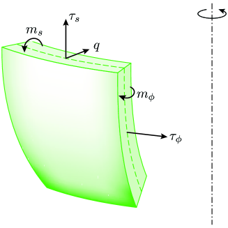
Figure 2: (Color online) Tensions and bending moments acting on the faces of a membrane patch

Figure 2 shows on which faces of a membrane patch the tensions and bending moments act. Figure 2 also shows an additional transverse shear tension $q$ which acts on the top (and bottom) side of the patch. It is constitutively undefined in our model because we did not incorporate deformations in which the capsule’s cross section gets sheared (i.e. fibers normal to the midsurface get rotated). However, the transverse shear tension is necessary to achieve force and moment equilibrium. Note that there does not act any transverse shear tension on the right side of the patch because of the assumption of axisymmetric, torsionless deformation.

II.4 Equilibrium Conditions

Besides the geometric relations and constitutive equations presented so far, conditions of force and moment equilibrium are needed to close the problem. These are three differential equations for tangential and normal force equilibrium and moment equilibrium, which take the form Libai1998 ; Pozrikidis2003

$$0 =-\frac{\cos\psi}{r}\,\tau_{\phi}+\frac{1}{r}\,\frac{\mathrm{d}(r\,\tau_{s})}{\mathrm{d}s}-\kappa_{s}\,q,$$ (11)

$$0 =-p+\kappa_{\phi}\,\tau_{\phi}+\kappa_{s}\,\tau_{s}+\frac{1}{r}\,\frac{\mathrm{d}(r\,q)}{\mathrm{d}s},$$ (12)

$$0 =\frac{\cos\psi}{r}\,m_{\phi}-\frac{1}{r}\frac{\mathrm{d}(r\,m_{s})}{\mathrm{d}s}-q,$$ (13)

in the absence of external tangential force and torque densities and for a constant pressure $p$ inside the capsule.

III Principle of Stationary Energy

III.1 Variation of Energy Functionals

Another approach to find stable configurations of capsules for fixed but altered volume $V\neq V_{0}$ is to minimize the functional of stored elastic energy $F=\int w_{S}\;\mathrm{d}A_{0}$ by calculus of variations. The constraint of fixed capsule volume $V$ is handled by introducing a Lagrange multiplier $p$ and extremizing the enthalpy $G=F-p\,V$ instead. The principle of stationary total energy Libai1998 states that the solutions of the equilibrium conditions (11) to (13) with given pressure $p$ render the enthalpy $G$ stationary.

In the case at hand, this can be verified by using the standard procedure of calculus of variations. Using $\mathrm{d}A_{0}=2\,\pi\,r_{0}\,\mathrm{d}s_{0}$ for the area element of the undeformed midsurface and $V=\int\pi\,r^{2}\;\mathrm{d}z=\int\pi\,r^{2}\,\sin\psi\;\mathrm{d}s=\int\pi\,r^{2}\,\lambda_{s}\,\sin\psi\;\mathrm{d}s_{0}$ as an integral expression for the capsule volume, we arrive at the enthalpy

$$G=\int_{0}^{L_{0}}\left(2\pi\,r_{0}\,w_{S}-p\,\pi\,r^{2}\,\lambda_{s}\,\sin\psi\right)\;\mathrm{d}s_{0},$$ (14)

for which we have to find stationary points. The Euler-Lagrange equations are derived in appendix A and turn out to be

$$0 = \frac{\cos\psi}{r}\,m_{\phi}-\frac{1}{r}\,\frac{\mathrm{d}(r\,m_{s})}{\mathrm{d}s}-q$$ (15)

$$0 = \frac{1}{r}\,\frac{\mathrm{d}(r\,\tau_{s})}{\mathrm{d}s}-\frac{\cos\psi}{r}\,\tau_{\phi}-\kappa_{s}\,q$$ (16)

$$q = -\tau_{s}\,\tan\psi+\frac{1}{2}\,p\,\frac{r}{\cos\psi}.$$ (17)

They coincide with the general equations of tangential force and moment equilibrium (11) and (13), but the normal force equilibrium equation (12) is replaced by the algebraic expression (17) for $q$. Instead of three differential equations in the general case, we now end up with only two differential equations and one algebraic relation. This means we have found a first integral of the general equations of equilibrium (which is only valid for capsules with spherical resting shape under uniform pressure). Inserting the algebraic expression (17) into the differential equation (12) for $q$ confirms that the solution found here satisfies the general equations of force equilibrium.

III.2 Shapes with Opposite Sides in Contact

Figure 3: (Color online) Ansatz for the configuration with opposite sides in contact. Along the contour, the important coordinates $s_{0}=L_{c}$ and $s_{0}=L_{0}/2$ are marked.

Among the solutions for negative pressure, unphysical solutions that exhibit self-intersection can occur. For two-dimensional shells with circular resting shape (cylinder, ring), Flaherty et al. addressed this problem in Flaherty1972 . They found that the opposite sides of an elastic ring touch at one point when the negative pressure reaches a certain threshold $p_{c1}$. Lowering the pressure further, the curvature at the point of contact decreases until it finally becomes zero at a second critical pressure $p_{c2}$. For pressures lower than $p_{c2}$, the contact area is a straight-line segment, which increases in length with decreasing pressure.

In order to generalize these results to three-dimensional spherical shells, we make the ansatz of a top/down symmetric deformed configuration with flat circular areas around the poles in contact with each other, see figure 3. Considering only top/down symmetric solutions, it is sufficient to set up the energy functional for the lower hemisphere only. The flat part with $0\leq s_{0}\leq L_{c}$, is referred to as part I, and the remaining part with $L_{c}\leq s_{0}\leq{L_{0}}/{2}$ as part II. In order to treat variations with respect to the boundary $L_{c}$ between parts I and II properly, the enthalpy functional is split up into two corresponding parts

$$G =W-p\,V-\mu\,\Delta z$$

$$={\int_{0}^{L_{c}}\mathrm{d}s_{0}\big{(}2\pi\,r_{0}\,w_{S}\big{)}}$$ (18)

$$+{\int_{L_{c}}^{L_{0}/2}\mathrm{d}s_{0}\left(2\pi\,r_{0}\ w_{S}-p\,\pi\,r^{2}\,\sin\psi\,\lambda_{s}-\mu\,\lambda_{s}\,\sin\psi\right)},$$

where the volume constraint and the condition $0=\Delta z=\int\mathrm{d}z=\int\lambda_{s}\,\sin\psi\;\mathrm{d}s_{0}$ are already incorporated via the Lagrange multipliers $p$ and $\mu$.

Performing the first variation involves the following problems: In part I, the function $r(s_{0})$ must be varied, and in part II the functions $r(s_{0})$ and $\psi(s_{0})$. Additionally, the integral boundary $L_{c}$ must be varied, which yields continuity conditions at $s_{0}=L_{c}$. The results can be summarized as follows.

In part I, we obtain one Euler-Lagrange equation

$$\frac{\partial(r\,\tau_{s})}{\partial s}=\tau_{\phi}\qquad\text{for}\quad s_{0}\in[0,\,L_{c}].$$ (19)

In part II we obtain a system of two Euler-Lagrange equations

$$0 =\frac{\cos\psi}{r}\,m_{\phi}-\frac{1}{r}\,\frac{\partial(r\,m_{s})}{\partial s}-q$$ (20)

$$0 =\frac{1}{r}\,\frac{\partial(r\,\tau_{s})}{\partial s}-\frac{\cos\psi}{r}\,\tau_{\phi}-\kappa_{s}\,q$$ (21)

$$\quad q =-\tau_{s}\,\tan\psi+\frac{1}{2}\,p\,\frac{r}{\cos\psi}+\frac{\mu}{2\pi}\,\frac{1}{r\,\cos\psi}$$ (22)

for $s_{0}\in[L_{c},\,L_{0}/2]$. The Euler-Lagrange equations for part II are very similar to those obtained above for non-intersecting shapes, except for the term $\frac{\mu}{2\pi}\,\frac{1}{r\,\cos\psi}$ in the algebraic expression for $q(s_{0})$. Nevertheless, it can be easily shown that relation (22) also satisfies the general equation (12), although it differs from the previous solution by the additional term with the Lagrange multiplier $\mu$.

In order to fit the solutions of part I and II together, continuity conditions must be derived, which arise from the variation with respect to the integral boundary $L_{c}$. It turns out that most quantities of interest are continuous at $s_{0}=L_{c}$, namely $r$, $z$, $\psi$, $\lambda_{i}$, $\kappa_{i}$, $\tau_{i}$, $m_{i}$ where an index $i$ stands for $s$ or $\phi$. Only for the transverse shear tension $q$ no continuity condition derives because of the lack of a constitutive relation between the shear tension $q$ and elastic deformations in the present formulation. We just know that the value $q(L_{c})$ depends via the algebraic relation (22) on the Lagrange multiplier $\mu$.

IV Shape Equations

The shape of the deformed capsule is governed by the equilibrium conditions, constitutive equations and geometric relations presented above. They can be rearranged to form a system of first order differential equations, known as the shape equations,

$$r^{\prime}(s_{0}) =\lambda_{s}\,\cos\psi$$ (23)

$$z^{\prime}(s_{0}) =\lambda_{s}\,\sin\psi$$

$$\psi^{\prime}(s_{0}) =\lambda_{s}\,\kappa_{s}$$

$$\tau_{s}^{\prime}(s_{0}) =\lambda_{s}\left(\cos\psi\,\frac{\tau_{\phi}-\tau_{s}}{r}+\kappa_{s}\,q\right)$$

$$m_{s}^{\prime}(s_{0}) =\lambda_{s}\left(\cos\psi\,\frac{m_{\phi}-m_{s}}{r}-q\right)$$

$$q^{\prime}(s_{0}) =\lambda_{s}\left(-\kappa_{s}\,\tau_{s}-\kappa_{\phi}\,\tau_{\phi}-\cos\psi\,\frac{q}{r}+p\right).$$

The first three equations in this system follow from the geometric relations (1) and (2) (without index “$0$”) and the last three from the equilibrium conditions (11) to (13). The change of variables from $s$ to $s_{0}$ was accomplished by the relation $\mathrm{d}s=\lambda_{s}\,\mathrm{d}s_{0}$, see (5). Usage of the algebraic expression (17) would reduce this system by one equation, but turns out to be numerically impractical because of singularities when $\psi$ approaches $\pi/2$.

In order to close the above system of shape equations, all functions appearing on the right hand side must be expressed in terms of the basic functions $r$, $z$, $\psi$, $\tau_{s}$, $m_{s}$ and $q$. Exploiting geometrical relations, the definitions of the strains and the constitutive equations, we find the set of relations

$$\begin{aligned} \kappa_{\phi}&=\frac{\sin\psi}{r},&\lambda_{s}&=(1-\nu^{2})\,\lambda_{\phi}\,\frac{\tau_{s}}{E\,H_{0}}-\nu(\lambda_{\phi}-1)+1,\\ \lambda_{\phi}&=\frac{r}{r_{0}},&\tau_{\phi}&=\frac{E\,H_{0}}{1-\nu^{2}}\,\frac{1}{\lambda_{s}}\big{(}(\lambda_{\phi}-1)+\nu\,(\lambda_{s}-1)\big{)},\end{aligned}$$

$$\begin{aligned} K_{\phi}&=\frac{\sin\psi-\sin\psi_{0}}{r_{0}},&K_{s}&=\frac{1}{E_{B}}\,\lambda_{\phi}\,m_{s}-\nu\,K_{\phi},\\ m_{\phi}&=E_{B}\,\frac{1}{\lambda_{s}}\big{(}K_{\phi}+\nu\,K_{s}\big{)},&\kappa_{s}&=\frac{K_{s}+\kappa_{s_{0}}}{\lambda_{s}},\end{aligned}$$ (24)

which close the system (23).

After changing variables from $s$ to $s_{0}$, the boundary conditions for a closed capsule without kinks at its poles are $r(0)=r(L_{0})=z(0)=\psi(0)=0$ and $\psi(L_{0})=\pi$, while the spherical reference shape satisfies (3) and (4). These boundary conditions cannot be directly used to determine boundary values for all strains and curvatures using (24) because some of the resulting expressions are ill-defined as ratio of two vanishing quantities. These boundary values can be evaluated analytically using L’Hôspital’s rule and symmetry arguments (physically significant functions should be either odd or even along the extended contour $s_{0}\in[-L_{0},\,L_{0}]$) in the limits $s_{0}\rightarrow 0$ and $s_{0}\rightarrow L_{0}$. Using this procedure boundary values at $s_{0}=0$ and $s_{0}=L_{0}$ can be written as

$$\lambda_{s} =\lambda_{\phi}=\frac{E\,H_{0}}{E\,H_{0}-\tau_{s}(1-\nu)}, q^{\prime} =\lambda_{s}\left(\frac{p}{2}-\kappa_{s}\,\tau_{s}\right),$$ (25)

$$\kappa_{s} =\kappa_{\phi}=\frac{m_{s}}{E_{B}\,(1+\nu)}+\frac{1}{R_{0}\,\lambda_{s}}, \tau_{s}^{\prime} =m_{s}^{\prime}=0.$$

Now, the system (23) can be solved numerically. In order to introduce dimensionless quantities, we choose $R_{0}$ as the length unit and $E\,H_{0}$ as the tension unit. A simple shooting method and a multiple shooting method numrec ; stoer , both with parameter tracing, were used to compute capsule shapes for progressively lowered pressure $p<0$.

For top/down symmetric configurations it is sufficient to integrate from the south pole $s_{0}=0$ to the equator $s_{0}=L_{0}/2$. In this case, the boundary conditions $r(0)=0$, $z(0)=0$, $\psi(0)=0$, $q(0)=0$, $\psi(L_{0}/2)=\pi/2$ and $q(L_{0}/2)=0$ must be satisfied. Whereas the conditions concerning $r$, $z$ and $\psi$ are obvious from geometry, the condition $q(0)=0$ holds because of the algebraic relation (17), and $q(L_{0}/2)=0$ because of the symmetry of the configuration: If $q(L_{0}/2)\neq 0$, the lower hemisphere would pull the upper one to the inside (or outside, depending on the sign of $q(L_{0}/2)$), which contradicts the top/down symmetry.

For solutions that are not top/down symmetric, we use shooting to a fitting point numrec because it is numerically impractical to integrate into a removable singularity. The appropriate boundary conditions are $r(0)=0$, $z(0)=0$, $\psi(0)=0$, $q(0)=0$, $r(L_{0})=0$, $\psi(L_{0})=\pi$ and $q(L_{0})=0$ in this case. The apparent problem that there are seven boundary conditions to a system of six first order differential equations is resolved by the algebraic relation (17). It effectively renders one of the boundary conditions to $q$ obsolete (in other words, the differential equation for $q$ with both boundary conditions concerning $q$ is obsolete, which leads to a system of five differential equations with five boundary conditions).

In the case of top/down symmetric configurations with opposite sides in contact, the solutions of part I and II must be fitted together according to the continuity conditions. In part I, the only degree of freedom is the function $r(s_{0})$ since $z(s_{0})=\psi(s_{0})=0$ because of the geometrical restrictions. The shape equations for part I can be obtained from the equilibrium condition (19), together with constitutive and geometric relations,

$$r^{\prime}(s_{0})= \lambda_{s}$$ (26)

$$\lambda_{s}^{\prime}(s_{0})= \frac{(1+\nu)}{R_{0}}\;\frac{\cos(\frac{s_{0}}{R_{0}})-1}{\sin(\frac{s_{0}}{R_{0}})}+\frac{r}{R_{0}^{2}\,\sin^{2}(\frac{s_{0}}{R_{0}})}$$

$$-\frac{\lambda_{s}\,\cot(\frac{s_{0}}{R_{0}})}{R_{0}}.$$

For reasons of symmetry, $\lambda_{s}(s_{0})$ must be an even function along the extended contour $s_{0}\in(-L_{0},\,L_{0})$. Therefore, $\lambda_{s}^{\prime}(0)=0$. The boundary condition for this part of the shape equations is $r(0)=0$. The stretch at the pole, $\lambda_{s}(0)$, is free and serves as a shooting parameter.

After a numerical solution of (26) has been found, the Hookean constitutive equations can be used to calculate the tension $\tau_{c}\equiv\tau_{s}(L_{c})$ and bending moment $m_{c}\equiv m_{s}(L_{c})$, which serve together with $r_{c}\equiv r(L_{c})$ as initial values for the integration on part II. The shape equations for part II can be adopted from (23). Only the boundary conditions must be changed to $r(L_{c})=r_{c}$, $z(L_{c})=0$, $\psi(L_{c})=0$, $\tau_{s}(L_{c})=\tau_{c}$, $m_{s}(L_{c})=m_{c}$, $z(L_{0}/2)=0$, $\psi(L_{0}/2)=\pi/2$ and $q(L_{0}/2)=0$. The shooting parameters to satisfy the three conditions at the far end are $\lambda_{s}(0)$, $q(L_{c})$ and $L_{c}$.

In the case of top/down asymmetric configurations with opposite sides in contact, we assume the region in contact to be a spherical cap with radius $R$. A region $0\leq s_{0}\leq L_{c}$ around the south pole has to change its curvature from $1/R_{0}$ to $-1/R$ (note the sign change) to match a region $L_{0}-L_{c2}\leq s_{0}\leq L_{0}$ around the north pole. We allow the region around the south pole to contract in the meridional direction by the factor $\lambda_{s}(s_{0})=\lambda_{d}$ (constant on $0\leq s_{0}\leq L_{c}$). The region around the north pole is allowed to contract by the factor $\lambda_{s}(s_{0})=\lambda_{t}$ (constant on $L_{0}-L_{c2}\leq s_{0}\leq L_{0}$) which may be different from $\lambda_{d}$. Since the deformed configurations of these two regions have to match exactly, we have the constraint $L_{c2}=L_{c}\,\lambda_{d}/\lambda_{t}$.

Thus, the shape of the contact region of the deformed capsule is determined by the four parameters $R$, $L_{c}$, $\lambda_{b}$ and $\lambda_{t}$. The shape of the non-contacting part of the capsule is again described by the shape equations (23). Since it is a system of six equations, and we have four additional parameters that are not known a priori, we are able to satisfy ten continuity conditions in total. That is just enough for the most important quantities $r$, $z$, $\psi$, $\tau_{s}$ and $m_{s}$ at both ends $L_{c}$ and $L_{0}-L_{c2}$ of the integration interval.

The explicit boundary conditions for the shape equations (23) are given by

$$\textstyle r(L_{c}) =\textstyle R\,\sin(L_{c}\,\lambda_{d}/R)$$ (27)

$$\textstyle z(L_{c}) =\textstyle R\,(\cos(L_{c}\,\lambda_{d}/R)-1)$$

$$\textstyle\psi(L_{c}) =\textstyle-L_{c}\,\lambda_{d}/R$$

$$\textstyle\tau(L_{c}) =\textstyle\frac{EHo}{1-\nu^{2}}\frac{1}{\lambda_{\phi}}(\lambda_{d}-1+\nu(\lambda_{\phi}-1))$$

$$\textstyle m_{s}(L_{c}) =\textstyle E_{B}\frac{1}{\lambda_{\phi}}(-\lambda_{d}/R-1/R_{0}+\nu(-\lambda_{\phi}/R-1/R_{0}))$$

$$\textstyle\text{with}\quad\lambda_{\phi} =\textstyle R\,\sin(L_{c}\,\lambda_{d}/R)/(R_{0}\,\sin(L_{c}/R_{0}))$$

for the starting point and

$$\textstyle r(L_{0}-L_{c2}) =\textstyle R\,\sin(L_{c}\,\lambda_{d}/R)$$ (28)

$$\textstyle z(L_{0}-L_{c2}) =\textstyle R\,(\cos(L_{c}\,\lambda_{d}/R)-1)$$

$$\textstyle\psi(L_{0}-L_{c2}) =\textstyle-L_{c}\,\lambda_{d}/R+\pi$$

$$\textstyle\tau(L_{0}-L_{c2}) =\textstyle\frac{EHo}{1-\nu^{2}}\frac{1}{\lambda_{\phi}}(\lambda_{t}-1+\nu(\lambda_{\phi}-1))$$

$$\textstyle m_{s}(L_{0}-L_{c2}) =\textstyle E_{B}\frac{1}{\lambda_{\phi}}(\lambda_{t}/R-1/R_{0}+\nu(\lambda_{\phi}/R-1/R_{0}))$$

$$\textstyle\text{with}\quad\lambda_{\phi} =\textstyle R\,\sin(L_{c2}\,\lambda_{t}/R)/(R_{0}\,\sin(L_{c2}/R_{0}))$$

for the end point of integration.

Note that taking $\lambda_{s}$ to be constant in the regions in contact is a strong simplification. A more involved theory would incorporate equations similar to (26) to determine the in-plane-displacements. However, we observed that the solution branches produced with this simplified method fit neatly in the bifurcation diagrams.

V Bifurcation Behavior

As the surface Young modulus $E\,H_{0}$ serves as the tension unit, there are only two elastic parameters left to vary, the Poisson ratio $\nu$ and the dimensionless bending modulus

$$\tilde{E}_{B}\equiv\frac{E_{B}}{R_{0}^{2}\,E\,H_{0}}=\frac{H_{0}^{2}}{12(1-\nu^{2})R_{0}^{2}}.$$ (29)

where we used (8) for the bending modulus of elastic plates. We will present bifurcation diagrams for a Poisson ratio of $\nu=0.5$ and dimensionless bending moduli of $\tilde{E}_{B}=0.01$ and $0.001$. These values correspond to relative shell thicknesses of $H_{0}/R_{0}=0.3$ and $0.095$, respectively.

V.1 Spherical Solution Branch

The trivial branch of spherical solutions (branch 1 in the bifurcation diagrams below) can be calculated analytically because of its high symmetry. Solving the equilibrium equations (11) to (13) for a sphere with radius $R$, it is straightforward to show that these equations reduce to the modified Laplace-Young equation

$$p=2\,\kappa\,\tau,$$ (30)

with $\kappa=1/R$ the isotropic curvature and $\tau\equiv\tau_{s}=\tau_{\phi}$ the isotropic tension. The Laplace-Young equation determines the new radius of the capsule for given pressure. Using the Hookean constitutive relation to express $\tau$ in terms of the isotropic stretch $\lambda_{s}=\lambda_{\phi}=R/R_{0}$, this condition can be rewritten as

$$R^{2}-\frac{2\,EH_{0}}{p\,(1-\nu)}\,(R-R_{0})=0.$$ (31)

The solution to this quadratic equation is the radius-pressure relation of the spherical branch (called branch 1 below)

$$R_{1}=\frac{EH_{0}}{p\,(1-\nu)}\pm\sqrt{\left(\frac{EH_{0}}{p\,(1-\nu)}\right)^{2}-\frac{2\,EH_{0}}{p\,(1-\nu)}\,R_{0}},$$ (32)

where the $+$ branch holds for $p<0$ and the $-$ branch for $p>0$, which can easily be inferred from requiring $\lim_{p\rightarrow 0}R=R_{0}$. This radius-pressure relation determines the deformed configuration completely, and all physical properties, like volume, strains, tensions and stored elastic energy, can be calculated in turn.

In the following we focus on buckling shapes for negative pressure $p<0$. For positive pressure $p>0$, where capsules are stretched, the spherical branch 1 represents the only equilibrium shape.

V.2 Stability Criteria

We have shown that the equations of force and moment equilibrium render the functional of total energy stationary. When the shape equations are solved for negative pressure, various solution branches with reduced capsule volume $V<V_{0}$ can be found, which can represent local minima or maxima of the energy functional. We display the total energy or enthalpy of each solution branch in an energy bifurcation diagram as a function of the capsule volume $V$ or the pressure $p$, respectively. The principle of minimal total energy allows us to determine the globally stable branch as the branch of minimal energy among all stationary shapes. Shape transitions such as buckling occur where two branches intersect.

If the capsule volume is given, the stored elastic energy

$$F=\int_{0}^{L_{0}}2\pi\,r_{0}\,w_{S}\;\mathrm{d}s_{0}$$ (33)

must be minimal. This criterion has experimental significance if the capsule volume cannot change because the encapsulated liquid is incompressible and the membrane is impermeable. In cases of a semipermeable capsule membrane, it is also reasonable to consider the volume fixed because the relaxation into the equilibrium shape happens on much shorter time scales than the diffusion of the inner liquid through the membrane. In the corresponding bifurcation diagram we display the stored elastic energy $F$ as a function of the volume $V$.

On the other hand, if the capsule is filled and surrounded by gases, the pressure difference $p$ is prescribed rather than the capsule volume. In this case, configurations with minimal enthalpy

$$G=F-p\,V=\int_{0}^{L_{0}}\left(2\pi\,r_{0}\,w_{S}-p\,\pi\,r^{2}\,\lambda_{s}\,\sin\psi\right)\;\mathrm{d}s_{0}$$ (34)

are energetically preferable. In the corresponding bifurcation diagram we display the elastic enthalpy $G$ as a function of the pressure $p$. Note that $G(p)$ is the Legendre transform of $F(V)$, since the relation $p=\mathrm{d}F/\mathrm{d}V$ holds (which was verified numerically for all solution branches presented here). Solution branches that lie lowest in the $F(V)$ bifurcation diagrams need not necessarily coincide with the lowest branches in the $G(p)$ diagrams.

Finally, it is also useful to analyze the relation between pressure $p$ and volume $V$ for stationary capsule shapes. Branches that exhibit an unusual pressure-volume relation with $\mathrm{d}p/\mathrm{d}V<0$ are inherently unstable if the pressure is given instead of the volume Balloons . To see that, we consider a water filled capsule connected to a reservoir of water. The pressure in this system can be prescribed. Now, if we try to change the capsule volume by lowering the pressure by an amount $\mathrm{d}p<0$, the capsule grows by an amount $\mathrm{d}V>0$, i.e. water flows from the reservoir into the capsule. The loss of water in the reservoir typically leads to an even lower pressure and thus, the equilibrium is unstable with repsect to volume changes. This instability is also reflected by a negative second derivative of the free energy, $d^{2}F/dV^{2}=\mathrm{d}p/\mathrm{d}V<0$ and a horizontal $p(V)$ curve with $dp/dV=0$ marks the onset of such an instability.

Therefore, we have three criteria of stability for capsule shapes:

• minimal energy $F$ for fixed capsule volume $V$,

• minimal enthalpy $G$ for fixed pressure $p$, and

• a monotonously decreasing pressure-volume relation $\mathrm{d}p/\mathrm{d}V<0$ is sufficient for an unstable shape for fixed pressure. Thus, the criterion $\mathrm{d}p/\mathrm{d}V\geq 0$ is only a necessary condition for stability: Configurations with $\mathrm{d}p/\mathrm{d}V\geq 0$ can still be unstable with respect to deformation modes which do not change the volume.

In fact, criterion (iii) can be generalized by using a general bifurcation theorem that has been proven in Ref. Maddox87 . This allows us to make a further statement about the instability of shapes beyond points where a monotonously decreasing $p(V)$ curve becomes vertical: If the $p(V)$ curve at such a point is open to the left, i.e., the following lower part of the $p(V)$ curve has again a positive slope $dp/dV>0$, this lower part must also be unstable. Furthermore, this is an instability with respect to a volume-preserving mode. This generalization also demonstrates that a positive slope $\mathrm{d}p/\mathrm{d}V\geq 0$ is not sufficient for stability.

V.3 Bifurcation Diagrams

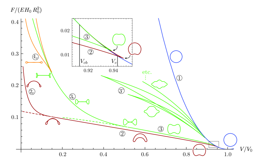
Figure 4: (Color online) Bifurcation diagram for given volume of a capsule with $\tilde{E}_{B}=0.001$. On the dashed lines of branch 2 and 3, the capsule intersects itself. Branch 3’ continues winding up in the diagram, as indicated by the "etc …".

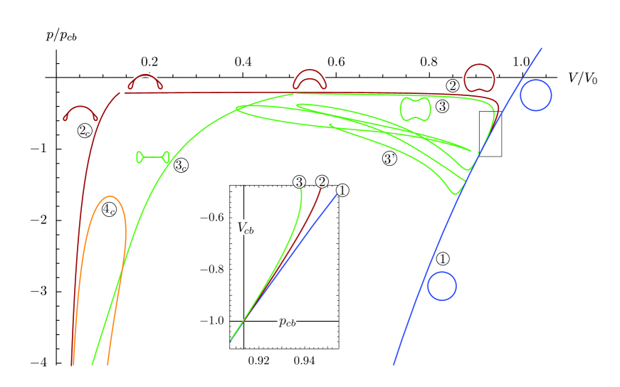
Figure 5: (Color online) Pressure-volume relation of a capsule with $\tilde{E}_{B}=0.001$

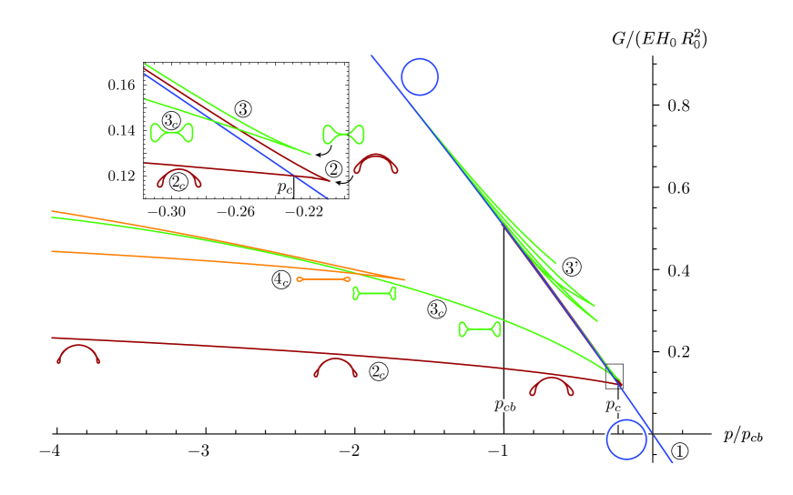
Figure 6: (Color online) Bifurcation diagram for given pressure of a capsule with $\tilde{E}_{B}=0.001$.

Branch	Configuration	Example
1	spherical
2	simply buckled (asymmetric)
2’	asymmetrically crumpled
$2_{c}$	simply buckled with contact
3	symmetrically buckled
3’, 3”	symmetrically crumpled	,
$3_{c}$, $4_{c}$	symmetrically buckled with contact	,

Table 1: Denomination of different branches in bifurcation diagrams. Branches are classified according to the number of bulges as buckled (one or two bulges) or crumpled (more than two bulges, names with primes) and according to top/down mirror-symmetry (shapes 1,3,4 are top-down symmetric, shapes 2 are asymmetric). Shapes with subscript $c$ exhibit contact of originally opposite sides; shape $3_{c}$ develops an additional dimple at the sides as opposed to shape $4_{c}$ (for $\tilde{E}_{B}=0.001$).

With these criteria of stability, we analyze the bifurcation behavior of elastic capsules by investigating the different branches in three types of bifurcation diagrams: 1) In the $F(V)$ diagram we study buckling by reducing the capsule volume by using criterion (i). 2) In the $p(V)$ diagram we can identify unstable shapes as monotonously decreasing branches $\mathrm{d}p/\mathrm{d}V<0$ according to criterion (iii). 3) In the $G(p)$ diagram the Legendre transform $G(p)=F(V(p))-pV(p)$ allows us to investigate buckling under negative pressure according to criterion (ii).

The nomenclature of solution branches is summarized in table 1. In particular, we will compare our results to classical buckling theory Pogorelov1988 ; LL7 ; Libai1998 , which predicts a critical negative buckling pressure

$$p_{cb}=-4\frac{E\,H_{0}^{2}}{R_{0}^{2}\,\sqrt{12(1-\nu^{2})}}=-4\sqrt{EH_{0}\,E_{B}}/R_{0}^{2}$$ (35)

for a spherical capsule. A corresponding critical volume can be obtained as

$$V_{cb}=\frac{4\pi}{3}\,(R_{1}(p_{cb}))^{3}$$ (36)

by using $p_{cb}$ in the radius-pressure relation (32) of the spherical branch 1.

We start with the bifurcation behavior of thin capsules with $\tilde{E}_{B}=0.001$, as shown in the diagrams 4 to 6. The $F(V)$ diagram (figure 4) reveals that the simply buckled configurations of branch 2 are energetically favorable for volumes $V<V_{c}$, where $V_{c}$ denotes a critical volume which is $V_{c}\approx 0.944\,V_{0}$ in this case. At the critical volume $V_{c}$, the spherical branch 1 and branch 2 of simply buckled configurations intersect. Note that this volume is larger than the critical volume $V_{cb}$ within classical buckling theory, which is $V_{cb}\approx 0.914\,V_{0}$ for this case. A shape transition between branches 1 and 2 at $V_{c}$ is discontinuous and involves an energy barrier. The upper part of branch 2 most likely represents the unstable transition state at $V=V_{c}$ between a spherical shape and the stable lower part of branch 2. Therefore, the energy barrier can be estimated by the energy difference between the upper and lower parts of branch 2 at $V=V_{c}$. More detailed stability considerations are given in section V.4 below.

For volumes $V<0.14\,V_{0}$, these configurations start to intersect themselves (dashed line). Simultaneously, a branch $2_{c}$ starts to exist with simply buckled configurations with opposite sides in contact. Although the method used to obtain this branch incorporated some simplifications, branches $2$ and $2_{c}$ connect neatly in the diagrams. In this domain, the ansatz with opposite sides in contact produces solutions with higher energies (branch $2_{c}$ compared to the dashed part of $2$), i.e. the self-intersecting solution branch raises in the $F(V)$ diagram when it is forced to satisfy the physical constraints.

For volumes $V<V_{c}$, the energetically next best configurations according to (i) are the symmetrically buckled ones of branch 3. They exhibit self-intersection for volumes $V<0.51\,V_{0}$. At higher energies, crumpled configurations can be found in branch 3’ that is connected to branch 3. They correspond to local minima, saddle points or maxima of the energy functional. Several more crumpled shapes can be found in this domain of the bifurcation diagram, but they are not shown for the sake of clarity. Similar crumpled configurations have been observed for small volumes in simulations using triangulated surface models, in particular at high compression rates Vliegenthart2011 . Trapping in metastable crumpled shapes can contribute to this behavior.

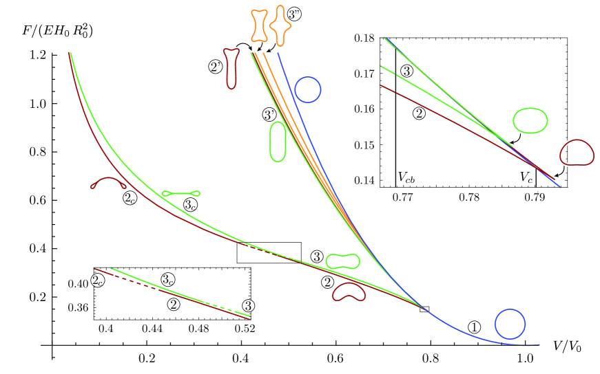
Figure 7: (Color online) Bifurcation diagram for given volume of a capsule with $\tilde{E}_{B}=0.01$. The dashed lines in the gaps between $2/2_{c}$ and $3/3_{c}$ could not be calculated numerically, but we expect some configurations to exist in these domains.

Figure 8: (Color online) Pressure-volume relation of a capsule with $\tilde{E}_{B}=0.01$. The dashed lines in the gaps between $2/2_{c}$ and $3/3_{c}$ could not be calculated numerically, but we expect some configurations to exist in these domains.

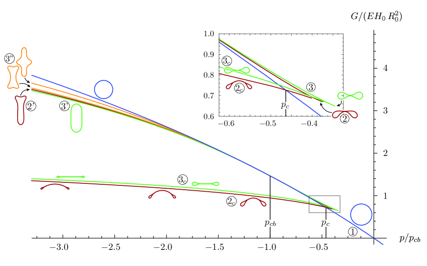
Figure 9: (Color online) Bifurcation diagram for given pressure of a capsule with $\tilde{E}_{B}=0.01$

For given pressure, the $p(V)$ diagram (figure 5) and $G(p)$ diagram (figure 6) can be analyzed in order to identify unstable solutions according to criteria (ii) and (iii). The simply and symmetrically buckled solutions of branches 2 and 3 (without contact of opposite sides) exhibit a negative slope in the $p(V)$ diagram. This means that they are mechanically unstable with respect to volume reducing deformations for given pressure according to criterium (iii), although they are most stable for fixed volume in the $F(V)$ diagram. According to the generalization of criterion (iii) based on Ref. Maddox87 also the lower part of branches 2 and 3, which lie beyond the turning point and have a positive slope in the $p(V)$ diagram at volumes $V>V_{cb}$, (see also inset in figure 5) are unstable, however, with respect to volume-preserving modes. The energy diagram $G(p)$ confirms this result; the unstable branches 2 and 3 lie above the trivial solution branch 1. On the other hand, the buckled configurations $2_{c}$ and $3_{c}$ with opposite sides in contact are mechanically stable again, with $\mathrm{d}p/\mathrm{d}V>0$, and $2_{c}$ is energetically preferable.

At the critical pressure $p_{c}\approx-0.23\,|p_{cb}|$, the spherical branch 1 and branch $2_{c}$ of simply buckled configurations with opposite sides in contact intersect in the $G(p)$ diagram, and shapes $2_{c}$ become energetically favorable for given pressure.

The negative critical pressure $|p_{c}|$ is much smaller than the classical buckling pressure $|p_{cb}|$, which is $p_{cb}\approx-0.126\,EH_{0}/R_{0}$ according to eq. (35). However, the classical buckling pressure fits very well to the point, where branches 2 and 3 emerge from the spherical solution branch in the $p(V)$ diagram (see inset in figure 5, where it is indicated by a horizontal line). The classical buckling pressure $p_{cb}$ is the pressure where the unbuckled spherical configuration 1 becomes unstable with respect to buckling LL7 ; Ru2009 , and a spontaneous transition to the unstable simply buckled branch 2 occurs.

At the critical pressure $p_{c}$, on the other hand, shape $2_{c}$ becomes energetically favorable as compared to the spherical branch 1. A shape transition between both branches at $p_{c}$ is discontinuous and involves an energy barrier. The upper unstable branch 2 of a simply buckled shape without contact most likely represents the transition state between a spherical shape and branch $2_{c}$ at $p=p_{c}$. Therefore, the energy barrier can be estimated by the energy difference between the upper unstable branch 2 and the lower stable branch $2_{c}$ at $p=p_{c}$.

The bifurcation diagrams for a thick capsule with $\tilde{E}_{B}=0.01$ (figures 7 to 9) look qualitatively similar. Again, the simply and symmetrically buckled solution branches 2 and 3, respectively, are energetically preferable for given volume, but exhibit a negative slope in the $p(V)$ diagram (figure 8), and are unstable and energetically unfavorable for given pressure.

For given volume $V$, the $F(V)$ diagram (figure 7) shows that the simply buckled configurations of branch 2 are energetically lower than spherical shapes for $V<V_{c}$ with a critical volume $V_{c}\approx 0.79\,V_{0}$, which is again larger than the critical volume $V_{cb}\approx 0.77\,V_{0}$ from classical buckling theory.

For given pressure $p$, the $G(p)$ diagram (figure 9) shows that simply buckled configurations $2_{c}$ with opposite sides in contact are energetically favorable as compared to spherical shapes of branch 1 for $p<p_{c}$, where the critical pressure is $p_{c}\approx-0.46\,|p_{cb}|$. Also for $\tilde{E}_{B}=0.01$, the negative critical pressure $|p_{c}|$ is much smaller than the classical buckling pressure $|p_{cb}|$, which is $p_{cb}\approx-0.4\,EH_{0}/R_{0}$ in this case and the classical buckling pressure fits to the point, where branch 2 emerges from the trivial spherical solution branch (see inset in figure 8, where it is indicated by a horizontal line).

For $\tilde{E}_{B}=0.01$, there is a visible gap between the buckled branches 2 and 3 and their respective continuations $2_{c}$ and $3_{c}$ with opposite sides in contact. This gap was already present in the diagrams for $\tilde{E}_{B}=0.001$, but much smaller. It is assumed to be closed by configurations with point contact of north and south pole. In the case of branch 3, an analogous behavior like that of elastic rings is expected Flaherty1972 . The curvature at the point of contact is expected to decrease, until it finally becomes zero and hence fulfills the continuity conditions for circular areas in contact. However, the shape equations when point contact of north and south pole is enforced turn out to be hard to solve numerically, because the transverse shear tension diverges at the poles.

At higher energies, there are again configurations with several bulges (branches 3’ and 3”). In the $F(V)$ diagram (figure 7), they lie lower than the trivial solution branch. In contrast to the results for the capsule with $\tilde{E}_{B}=0.001$, branch 3” does not have multiple turning points and is not connected to the continuation 3’ of the symmetrically buckled branch within the scope of our diagrams. However, branches 3’ and 3” might join at higher energies and lower pressures. Notably, these solution branches lie lower than branch 1 in the $G(p)$ diagram (figure 9), which is a qualitative difference to the results for $\tilde{E}_{B}=0.001$.

The $F(V)$ and $p(V)$ diagrams are in good agreement with previous work based on triangulated surface models: In Ref. Marmottant2011 , a $p(V)$ relation has been obtained, which also shows a uniform shrinkage of the capsule (our branch 1) for small volume reduction followed by a jump into an axisymmetric simply buckled configuration (our branch 2) with the same $p(V)$ behavior as branch 2. Furthermore, Ref. Quilliet2008 contains an $F(V)$ diagram in which the spherical and simply buckled solution branches are shown. They reveal qualitatively the same $F(V)$ relation as our branches 1 and 2.

V.4 Buckling Bifurcation

The key features of the bifurcation diagrams presented above are drawn schematically in figure 10. They allow to construct a complete picture of the bifurcation behavior at the buckling transition.

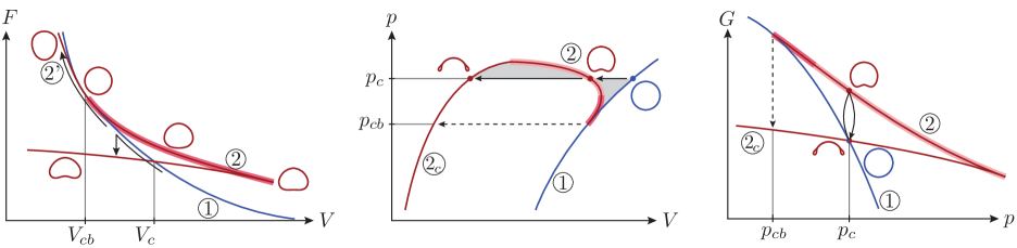
Figure 10: (Color online) Left: Schematic drawing of two different bifurcation phenomena (indicated by the arrows) for given volume $V<V_{c}$. Middle and right: Schematic drawing of a realistic buckling process for given pressure. The critical pressure $p_{c}$ is defined by the crossing of branches 1 and $2_{c}$ in the $G(p)$ diagram. As a consequence of the Legendre transformation, the two regions shaded gray in the $p(V)$ diagram have the same area at $p=p_{c}$ (Maxwell construction).

On the left of figure 10, two different bifurcation scenarios in the domain where branch 2 emerges from 1 are drawn schematically. We see that the part of branch 2 with an inward dimpled south pole emerges continuously from the spherical branch 1 and first runs to the right, i.e. to higher capsule volumes. After a turning point, the branch runs to the left, i.e. to lower capsule volumes, while the south pole buckles more and more inwards. The upper part of branch 2 up to the turning point (shaded dark red) lies at higher energies than the spherical branch and consists of unstable stationary shapes. This can be seen from the $p(V)$ diagram where it corresponds to the lower part of branch 2 beyond the vertical turning point and which are unstable with respect to a volume-preserving deformation mode according to the generalization of criterion (iii) Maddox87 .

Branch 2 intersects the spherical branch 1 at the critical volume $V=V_{c}$. For $V<V_{c}$ the lower part of branch 2 is the energetically preferable solution branch. A shape transition between branches 1 and 2 at $V_{c}$ is discontinuous. If the capsule wants to switch from the metastable branch 1 to 2 for $V<V_{c}$ (vertical arrow) an energy barrier must be overcome. The upper part of branch 2 represents the unstable transition states between a spherical shape and the stable lower part of branch 2. Therefore, the energy barrier can be estimated by the energy difference between the upper and lower parts of branch 2.

The behavior when branch 2’ emerges from the spherical branch 1 at the volume $V=V_{cb}$ is quite different. It emerges with egg-like configurations continuously from the trivial branch and runs directly to the left. If the capsule passes this point in the bifurcation diagram during a progressive reduction of its volume along the metastable branch 1, it is allowed to switch from branch 1 to 2’ continuously. Thus, there is no energy barrier to be overcome in this scenario, and the trivial branch is supposed to be unstable.

Details of a realistic buckling process for given pressure can be constructed from the $p(V)$ and $G(p)$ diagrams. The middle and right parts of figure 10 schematically show the key features concerning the simply buckled states 2 and $2_{c}$. The decreasing part of branch 2 with $\mathrm{d}p/\mathrm{d}V<0$ is mechanically unstable with respect to volume reduction (shaded light red). According to the generalization of criterion (iii) based on Ref. Maddox87 also the lower part of branch 2 (shaded dark red), which has a positive slope for a small volume range $V>V_{cb}$ in the $p(V)$ diagram, is unstable with respect to a volume-preserving deformation mode. It corresponds to the unstable upper branch 2 in the $F(V)$ diagram. In the $G(p)$ diagram both corresponding unstable parts of branch 2 join to give the energetically unfavorable upper branch.

Therefore, the spherical shapes of branch 1 become mechanically unstable at the classical buckling pressure $p_{cb}$, where the unstable branch 2 and branch 1 merge in the $p(V)$ diagram. Then, a small dimple caused by fluctuations or agitations can grow spontaneously and the capsule finally ends up in a fully collapsed stable configuration $2_{c}$ at the given pressure running along the dashed path in the $p(V)$ diagram. The same process is indicated in a schematic $G(p)$ diagram on the right of figure 10 as a dashed line.

Shape $2_{c}$ becomes energetically preferable already at a much smaller negative pressure $p_{c}$, i.e., $|p_{c}|<|p_{cb}|$, where branches 1 and $2_{c}$ intersect in the $G(p)$ diagram. A shape transition between branches 1 and $2_{c}$ at $p_{c}$ is discontinuous: Changing onto branch $2_{c}$ at $p=p_{c}$ does not correspond to a spontaneous snap-through into a fully buckled shape $2_{c}$ because shape $1$ remains mechanically (meta)stable in that region, because $\mathrm{d}p/\mathrm{d}V>0$ and no other branches are merging/intersecting in the $p(V)$ diagram at $p_{c}$. A finite dimple has to form by fluctuations or agitations to induce buckling, and this is associated with an energy barrier. The unstable transition state of this process can be the unstable shape 2 at the same pressure. This process is shown as a solid path in the $p(V)$ diagram. We note that, as a consequence of the condition of equal enthalpies $G$ at $p=p_{c}$, this solid path can be obtained by a Maxwell construction: At $p=p_{c}$, the two regions shaded gray in the $p(V)$ diagram have the same area.

We conclude this section by providing estimates for buckling pressures for some synthetic and biological capsules. For synthetic capsules made from typical soft materials we expect a Young’s modulus in the range $E\sim 100-1000\,{\rm MPa}$, thicknesses $H_{0}\sim 10-50\,{\rm nm}$, and micrometer sizes $R_{0}\sim 500\,{\rm nm}$, see for example Refs. Zoldesi2008 ; Fery2004 for different synthetic capsules. This results in typical classical buckling pressures $|p_{cb}|\sim 0.1-1\,{\rm GPa}$ (in accordance with measurements in Fery2004 ). Such materials have a small dimensionless bending modulus $\tilde{E}_{B}\sim 0.00005-0.001$ corresponding to thin shells, see figures 4, 5, and 6.

Many biological materials, such as virus capsids have very similar material characteristics but can be smaller: In Ref. Ru2009 $E=1\,{\rm GPa}$, $H_{0}=2\,{\rm nm}$, and $R_{0}=10\,{\rm nm}$ has been used for virus capsids, which gives similar dimensionless bending modulus $\tilde{E}_{B}\sim 0.004$ and a similar buckling threshold $|p_{cb}|=0.5\,{\rm GPa}$.

Somewhat different are soft biological capsules such as red blood cells with a shell made from lipid bilayers, which governs the bending rigidity. Red blood cells have a bending rigidity $E_{B}\sim 10\,k_{B}T$, an area stretching modulus $K\sim EH_{0}\sim 10\,{\rm\mu N/m}$ Park2011 , and sizes $R_{0}\sim 4\,{\mu m}$, which results in a smaller dimensionless bending modulus $\tilde{E}_{B}\sim 0.0005$ and a much smaller classical buckling threshold $|p_{cb}|\sim 0.2\,{\rm Pa}$ in accordance with the fact that red blood cell shapes are buckled at ambient conditions.

From our above result $p_{c}\approx 0.23\,p_{cb}$ for thin shells with $\tilde{E}_{B}\sim 0.001$, we expect critical values $|p_{c}|$, which are smaller by a factor of at least $5$ compared to the classical buckling pressure $|p_{cb}|$ for all of these capsules.

VI Analysis of Simply Buckled Shapes and Bending Modulus

Smaller bending resistances allow sharper bends in buckled configurations. Hence, the minimal radius of curvature $1/\kappa_{\rm edge}\equiv\min_{s}(1/\kappa_{s})$ (in $s$-direction along the contour), which occurs close to the edge of the indentation of a simply buckled shape 2 (see figure 12), should depend sensitively on the reduced bending resistance $\tilde{E}_{B}$ and represent an adequate observable to infer the reduced bending modulus $\tilde{E}_{B}$.

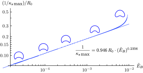
Figure 11: (Color online) Minimal radius of curvature $1/\kappa_{\rm edge}$ plotted against the reduced bending resistance $\tilde{E}_{B}$. Dots: Computed shapes for $V=0.8\,V_{0}$. Line: Power law fit for $\tilde{E}_{B}\leq 0.004$.

Figure 11 shows a double logarithmic plot of the minimal radius of curvature as a function of the reduced bending modulus. It was obtained from a series of simply buckled shapes with fixed volume $V=0.8\,V_{0}$. For bending moduli $\tilde{E}_{B}\leq 0.004$, a power law can be fitted to the data:

$$\frac{1}{\kappa_{\rm edge}}\sim R_{0}\,{\tilde{E}_{B}}^{0.2356}.$$ (37)

The power law (37) can be confirmed by a scaling argument, where we balance bending and stretching energies. We consider a small dimple with radius $r\ll R_{0}$ and depth $h$ as depicted in figure 12. The elastic energy is mainly located at the edge of this dimple, which spans the width $d\ll r$.

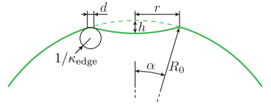
Figure 12: (Color online) Geometry of an axisymmetric dimple in a simply buckled shape 2.

Since the dimple is assumed to be mirror-inverted to its original shape, its radius and depth are determined by the angle $\alpha$ (see figure 12). To leading order, they are given by $r\sim R_{0}\,\alpha$ and $h\sim R_{0}\,\alpha^{2}$ respectively. By that, the volume change with respect to the unbuckled configuration is approximately $\Delta V\sim h\,r^{2}\sim R_{0}^{3}\,\alpha^{4}$.

The energies of bending and stretching are of the order

$$F_{b}\sim E_{B}\,\frac{\zeta^{2}}{d^{4}}\,r\,d\quad\text{and}\quad F_{s}\sim EH_{0}\,\frac{\zeta^{2}}{R_{0}^{2}}\,r\,d$$ (38)

respectively LL7 , where $\zeta$ is the typical radial displacement of the membrane near the edge of the dimple. Because the direction of the meridian changes about $\alpha$ within the width $d$, we have $\zeta\sim\alpha\,d\sim d\,(\Delta V/R_{0}^{3})^{1/4}$. The total elastic energy for a given volume reduction $\Delta V$ therefore takes the form

$$F\sim EH_{0}\frac{d^{3}\,r\,\Delta V^{1/2}}{R_{0}^{7/2}}+E_{B}\frac{r\,\Delta V^{1/2}}{d\,R_{0}^{3/2}}.$$ (39)

Minimizing the total elastic energy with respect to $d$ we find the equilibrium width of the dimple edge,

$$d\sim\left(\frac{E_{B}}{EH_{0}}R_{0}^{2}\right)^{1/4}\sim R_{0}\,\tilde{E}_{B}^{1/4},$$ (40)

which can also be written in the form $d\sim\sqrt{H_{0}\,R_{0}}$ as in ref. LL7 . Confining the directional change $\alpha$ of the meridian to a width $d$ of the edge of the indentation (see figure 12) results in an edge curvature

$$\kappa_{\text{edge}}\sim\frac{\alpha}{d}\sim\frac{\Delta V^{1/4}}{R_{0}^{7/4}}\,\tilde{E}_{B}^{-1/4}.$$ (41)

When the critical buckling pressure $|p_{c}|$ is small (compared to the pressure unit defined by $EH_{0}/R_{0}$), the unbuckled region outside the dimple remains roughly spherical with a radius close to the original radius $R_{0}$, as can be seen from eq. 31. Therefore,

$$\Delta V=V_{0}-V=(1-v)V_{0}$$ (42)

holds to a good approximation, where $v\equiv V/V_{0}$ is a reduced volume. Using this in (41), we find a scaling law

$$\kappa_{\text{edge}}\sim\frac{(1-v)^{1/4}}{R_{0}}\,\tilde{E}_{B}^{-1/4},$$ (43)

which is of the same form as the above fit (37) with an exponent $1/4$ matching the fit result $0.2356$ from (37) quite well.

It is evident from the assumption $d\ll r$, which corresponds to a sharp edge of the indentation, that the scaling law holds only for sufficiently small bending resistances, $\tilde{E}_{B}\leq 0.004$ in this case. The assumption $r\ll R_{0}$ implies that the scaling law holds for sufficiently small volume changes. Indeed, analyzing the scaling behavior for several capsule volumes using (43), we find that the fitted exponent matches the theoretical value $1/4$ very well for $V=0.9\,V_{0}$ or $0.8\,V_{0}$, but starts to deviate for $V=0.67\,V_{0}$ or $0.5\,V_{0}$, see table 2. We can also determine that the numerical prefactor in (43) is of the order of unity and only weakly volume dependent. In contrast to these findings for simply buckled shapes 2 without contact of opposite sides, we observe that $\kappa_{\text{edge}}$ is nearly independent of $\tilde{E}_{B}$ for buckled conformations of branch $2_{c}$ with opposite sides in contact.

reduced Volume $v$	prefactor $c$	exponent $b$
$0.9$	0.73	0.246
$0.8$	0.63	0.236
$0.75$	0.59	0.229
$0.67$	0.54	0.221
$0.5$	0.50	0.217

Table 2: Fit parameters for different capsule volumes. The fit model for the radius of curvature at the dimple edge is $1/\kappa_{\text{edge}}=c\,{(1-v)^{-1/4}}\,R_{0}\,{\tilde{E}_{B}}^{b}$, see eq. (43). For small volume changes, the theoretical exponent $1/4$ agrees best.

The results of the fits presented in table 2 could be used to quantitatively analyze experimental shapes of simply buckled elastic capsules without opposite sides in contact as shown, for example, in Refs. Fery2004 ; Zoldesi2008 ; Sacanna2011 ; Quilliet2008 , provided the radius of curvature at the edge of the dimple can be measured accurately. We note that the calculated shapes as shown in figure 11 are in qualitative agreement with some of the experimentally observed shapes Fery2004 ; Zoldesi2008 ; Sacanna2011 ; Quilliet2008 . From a measurement of the curvature at the edge of the buckling dimple $\kappa_{\rm edge}$ the dimensionless bending modulus $\tilde{E}_{B}=E_{B}/(R_{0}^{2}\,E\,H_{0})$ can be determined using (41) and the numerical prefactor from table 2. In combination with an independent measurement of Young’s modulus $E$, for example, via a measurement of the classical buckling pressure $p_{cb}$, this type of shape analysis provides a method to obtain the bending modulus of a capsule, which is hard to measure otherwise.

VII Conclusions

We applied nonlinear shell theory to the problem of axisymmetric deformations of an initially spherical capsule. The elastic properties of the capsule membrane were modeled with a quadratic strain-energy function. This approach to Hooke’s law allowed us to use the methods of force and moment equilibrium and a least-energy principle simultaneously.

Bifurcation diagrams for reduced capsule volume and negative pressure were presented. The least-energy principle gave information about the preferred configurations and allowed to obtain a complete picture of the transition into the fully buckled state. If the capsule volume is controlled, simply buckled configurations turned out to be energetically preferable below a certain critical volume $V_{c}$, but an energy barrier must be overcome in order to leave the trivial solution branch. The transition at $V_{c}$ is thus discontinuous. If the internal negative pressure is controlled, spherical shapes become mechanically unstable at the classical buckling pressure $p_{cb}$. However, buckled shapes with opposite sides in contact become energetically favorable at a much lower negative pressure $p_{c}$, i.e., $|p_{c}|<|p_{cb}|$. Also at controlled negative pressure, the transition at $p_{c}$ is discontinuous and involves an energy barrier. With the methods presented here, also configurations with opposite sides in contact could be computed and incorporated in the bifurcation diagrams; fully buckled configurations with opposite sides in contact (branch $2_{c}$ in the bifurcation diagrams) actually have the lowest energies at small volumes or low negative pressures and determine the critical pressure $p_{c}$.

For buckled shapes, the maximal curvature $\kappa_{\text{edge}}$ at the edge of inward buckled dimples was found to depend depend strongly on the ratio of bending resistance to surface Young modulus, with smaller ratios leading to sharper bends. A power law $\kappa_{\text{edge}}\propto(EH_{0}/E_{B})^{1/4}$ was found for sufficiently small bending resistances and sufficiently small volume changes. This relation may be used to analyze experimental shapes of buckled elastic capsules and extract the bending modulus of the capsule membrane from the capsule shape.

Appendix A Calculus of Variations

In this appendix we derive the first variation and the resulting Euler-Lagrange equations for the enthalpy functional

$$G=\int_{0}^{L_{0}}\left(2\pi\,r_{0}\,w_{S}-p\,\pi\,r^{2}\,\lambda_{s}\,\sin\psi\right)\;\mathrm{d}s_{0}.$$ (44)

The integrand has to be regarded as a function of $s_{0}$. In functions like $r(s)$, a change of variables from $s$ to $s_{0}$ can be performed by the function $s(s_{0})$ introduced in (5).

Two of the functions $r(s_{0})$, $z(s_{0})$ and $\psi(s_{0})$ determine the capsule configuration completely. As the integrand of (14) and the geometrical relations contain mainly $r$ and $\psi$, we choose $r(s_{0})$ and $\psi(s_{0})$ as the two basic fields. Variations $\delta r(s_{0})$ and $\delta\psi(s_{0})$ have to fulfill the boundary conditions

$$\delta r(0)=\delta r(L_{0})=0\quad\text{and}\quad\delta\psi(0)=\delta\psi(L_{0})=0.$$ (45)

The first variation $\delta G$ of $G[r,\,\psi]$ is obtained as

$$\delta G=\int_{0}^{L_{0}}\left(2\pi\,r_{0}\,\delta w_{S}-p\,\pi\,\delta(r^{2}\,\lambda_{s}\,\sin\psi)\right)\;\mathrm{d}s_{0}.$$ (46)

The variation $\delta w_{S}$ of the surface energy density introduces tensions and bending moments with the help of the constitutive equations (10),

$$\delta w_{S} =\frac{\partial w_{S}}{\partial e_{s}}\,\delta e_{s}+\frac{\partial w_{S}}{\partial e_{\phi}}\,\delta e_{\phi}+\frac{\partial w_{S}}{\partial K_{s}}\,\delta K_{s}+\frac{\partial w_{S}}{\partial K_{\phi}}\,\delta K_{\phi}$$

$$=\lambda_{\phi}\,\tau_{s}\,\delta e_{s}+\lambda_{s}\,\tau_{\phi}\,\delta e_{\phi}+\lambda_{\phi}\,m_{s}\,\delta K_{s}+\lambda_{s}\,m_{\phi}\,\delta K_{\phi}.$$ (47)

Now, the variations of the strains must be expressed in terms of $\delta r$, $\delta\psi$ and its derivatives with the help of strain definitions and geometrical relations,

$$e_{s} =\frac{r^{\prime}(s_{0})}{\cos\psi(s_{0})}-1 \Rightarrow \delta e_{s} =\frac{\delta r^{\prime}}{\cos\psi}+\lambda_{s}\,\tan\psi\,\delta\psi$$ (48)

$$e_{\phi} =\frac{r}{r_{0}}-1 \Rightarrow \delta e_{\phi} =\frac{1}{r_{0}}\,\delta r$$

$$K_{s} =\psi^{\prime}(s_{0})-\kappa_{s_{0}} \Rightarrow \delta K_{s} =\delta\psi^{\prime}$$

$$K_{\phi} =\frac{\sin\psi}{r_{0}}-\kappa_{\phi_{0}} \Rightarrow \delta K_{\phi} =\frac{\cos\psi}{r_{0}}\,\delta\psi.$$

In a similar fashion, the variation of the second term can be calculated as

$$\delta(r^{2}\,\lambda_{s}\,\sin\psi)=\delta(r^{\prime}\,r^{2}\,\tan\psi)\\ =2\,r\,\lambda_{s}\,\sin\psi\,\delta r+r^{2}\,\tan\psi\,\delta r^{\prime}+\frac{\lambda_{s}\,r^{2}}{\cos\psi}\,\delta\psi.$$ (49)

Inserting everything into (46), and sorting according to $\delta r$, $\delta r^{\prime}$, $\delta\psi$, $\delta\psi^{\prime}$ yields a rather long expression. Using integration by parts to transform $\delta r^{\prime}$ into $\delta r$ and $\delta\psi^{\prime}$ into $\delta\psi$ (note that the boundary terms vanish) results in the following result for the first variation of $G$,

$$\delta G=\int_{0}^{L_{0}}\!\!\!\!\mathrm{d}s_{0}\Big{(}\delta r\Big{\{}2\pi\,\lambda_{s}\,\tau_{\phi}-2\pi\,p\,r\,\lambda_{s}\,\sin\psi\\ -2\pi\,\frac{\mathrm{d}}{\mathrm{d}s_{0}}\!\!\Big{(}\frac{r\,\tau_{s}}{\cos\psi}\Big{)}+\pi\,p\,\frac{\mathrm{d}}{\mathrm{d}s_{0}}(r^{2}\,\tan\psi)\Big{\}}\\ +\delta\psi\Big{\{}2\pi\,r\,\tau_{s}\,\lambda_{s}\,\tan\psi+2\pi\,\lambda_{s}\,m_{\phi}\,\cos\psi\\ -\pi\,p\,\frac{\lambda_{s}\,r^{2}}{\cos\psi}-2\pi\,\frac{\mathrm{d}(r\,m_{s})}{\mathrm{d}s_{0}}\Big{\}}\Big{)}.$$ (50)

For a stationary shape, $\delta G=0$ for arbitrary variations $\delta\psi$ and $\delta r$, and the terms in curly braces have to vanish. This gives the Euler-Lagrange equations describing stationary states. Rearranging the term next to $\delta\psi$ by a change of variables $\mathrm{d}s=\lambda_{s}\,\mathrm{d}s_{0}$, we obtain

$$0 =\frac{\cos\psi}{r}\,m_{\phi}-\frac{1}{r}\,\frac{\mathrm{d}(r\,m_{s})}{\mathrm{d}s}-q$$ (51)

$$\text{with}\quad q =-\tau_{s}\,\tan\psi+\frac{1}{2}\,p\,\frac{r}{\cos\psi}.$$ (52)

which are eqs. (15) and (17) in the main text. With this definition of the transverse shear tension $q$, the term next to $\delta r$ can be simplified to

$$0=\frac{1}{r}\,\frac{\mathrm{d}(r\,\tau_{s})}{\mathrm{d}s}-\frac{\cos\psi}{r}\,\tau_{\phi}-\kappa_{s}\,q.$$ (53)

which gives eq. (16) in the main text.

References

- (1) W. Meier, Chem. Soc. Rev. 29, 295 (2000).
- (2) H. Rehage, M. Husmann, and A. Walter Rheol. Acta 41, 292 (2002).
- (3) E. Donath, G. Sukhorukov, F. Caruso, S. Davis, and H. Möhwald, Ang. Chem. Int. Ed. 37, 2201 (1998).
- (4) D. Barthès-Biesel, Curr. Opin. Coll. Interface Sci. 16, 3 (2011).
- (5) G. Pieper, H. Rehage, and D. Barthès-Biesel, J. Coll. Int. Sci. 202, 293 (1998).
- (6) S. Komura, K. Tamura, and T. Kato, Eur. Phys. J. E 18, 343 (2005).
- (7) P. Graf, R. Finken, and U. Seifert, Langmuir 22, 7117 (2006).
- (8) A. Fery, F. Dubreuil, and H. Möhwald, New J. Phys. 6, 18 (2004).
- (9) A. Fery and R, Weinkamer, Polymer 48, 7221 (2007).
- (10) C.I Zoldesi, I.L. Ivanovska, C. Quilliet, G.J.L. Wuite, and A. Imhof, Phys. Rev. E, 78, 051401 (2008).
- (11) C. Gao, E. Donath, S. Moya, V. Dudnik, and H. Möhwald, Eur. Phys. J. E 5, 21 (2001).
- (12) S. Sacanna, W.T.M. Irvine, L. Rossi and D.J. Pine, Soft Matter 7, 1545 (2011).
- (13) L.D. Landau and E.M. Lifshitz, Theory of Elasticity (Pergamon, NewYork, 1986).
- (14) C.Q. Ru, J. Appl. Phys. 105, 124701 (2009).
- (15) M. Blyth and C. Pozrikidis, Eur J. Mech. A Solids 23, 877 (2004).
- (16) L. Bauer, E.L. Reiss, and H.B. Keller, Comm. Pure Appl. Math. 23, 529 (1970).
- (17) G.A. Vliegenthart and G. Gompper, New J. Phys. 13, 045020 (2011).
- (18) C. Quilliet, C. Zoldesi, C. Riera, A. van Blaaderen and A. Imhof, Eur. Phys. J. E 27, 13 (2008).
- (19) P. Marmottant, A. Bouakaz, N. de Jong, C. Quilliet, J. A. S. A. 129, 1231 (2011).
- (20) A. Libai and J.G. Simmonds, The Nonlinear Theory of Elastic Shells, (Cambridge University Press, Cambridge, 1998).
- (21) C. Pozrikidis, Modeling and Simulation of Capsules and Biological Cells (Chapman and Hall/CRC, Boca Raton, 2003).
- (22) J.E. Flaherty, J.B. Keller, and S.I. Rubinow, SIAM J. Appl. Math. 23, 446 (1972).
- (23) W.H. Press, S.A. Teukolsky, W.T. Vetterling, and B.P. Flannery, Numerical Recipes (Cambridge University Press, New York, 2007).
- (24) J. Stoer and R. Bulirsch, Introduction to Numerical Analysis, (Springer, New York, 2010).
- (25) I. Müller and P. Strehlowm Rubber and Rubber Balloons: Paradigms of Thermodynamics (Springer, Berlin, 2004).
- (26) J. H. Maddocks, Arch. Rat. Mech. Anal. 99, 301 (1987).
- (27) A.V. Pogorelov, Bendings of Surfaces and Stability of Shells, (American Mathematical Society, Providence, 1988).
- (28) Y. Park, C. Best, T. Kuriabova, M.L. Henle, M.S. Feld, A.J. Levine, and G. Popescu, Phys. Rev. E 83, 051925 (2011).