Wavelet-Based Linear-Response Time-Dependent Density-Functional Theory
Abstract
Linear-response time-dependent (TD) density-functional theory (DFT) has been implemented in the pseudopotential wavelet-based electronic structure program BigDFT and results are compared against those obtained with the all-electron Gaussian-type orbital program deMon2k for the calculation of electronic absorption spectra of N2 using the TD local density approximation (LDA). The two programs give comparable excitation energies and absorption spectra once suitably extensive basis sets are used. Convergence of LDA density orbitals and orbital energies to the basis-set limit is significantly faster for BigDFT than for deMon2k. However the number of virtual orbitals used in TD-DFT calculations is a parameter in BigDFT, while all virtual orbitals are included in TD-DFT calculations in deMon2k. As a reality check, we report the x-ray crystal structure and the measured and calculated absorption spectrum (excitation energies and oscillator strengths) of the small organic molecule -cyclohexyl-2-(4-methoxyphenyl)imidazo[1,2-]pyridin-3-amine.
I Introduction
The last century witnessed the birth, growth, and increasing awareness of the importance of quantum mechanics for describing the behavior of electrons in atoms, molecules, and solids. One key to unlocking the door to widespread applications was the advent of scientific computing in the 1960s. New computational methods had to be developed — and continue to be developed — to make use of the increasing computational power. Wavelet-based methods are a comparative newcomer to the world of electronic structure algorithms (Refs. A99 ; G98 provide useful, if dated, reviews) but offer increasing accuracy for grid-based density-functional theory (DFT) calculations of molecular properties. Although DFT is a theory of the ground stationary state, excited states may be treated by the complementary time-dependent (TD) theory. This paper reports the first implementation of TD-DFT in a wavelet-based code — namely our implementation of linear response TD-DFT in the BigDFT bigdft program. TD-DFT results obtained with our implementation in BigDFT and with the Gaussian-type orbital (GTO) based program deMon2k deMon2k are compared and BigDFT is used to calculate and analyse the absorption spectrum of a recently-synthesized small organic molecule BMO11 .
Modern computing requires discretization and this has been historically treated in DFT and non-DFT ab initio abinitio electronic structure calculations by basis set expansions. Because the basis set is necessarily finite, electronic structure algorithms for solids and molecules have developed as refinements on physically-sensible zero-order systems, based upon the reasonable idea that fewer basis functions should be needed when the underlying physics is already approximately correct. Thus computations on solids used plane-wave basis sets partly because of analogies with the free-electron model of metals and partly for other reasons (ease of integral evaluation and Bloch’s theorem taking explicit account of crystal symmetry.) Similarly computations on molecules are typically based upon the linear combination of atomic orbital (LCAO) approximation to molecular orbitals, with split-valence, polarization, and diffuse functions added as needed to go beyond this crude first approximation. A key feature of finite-basis-set calculations has been the use of the variational principle in order to guarantee smooth convergence from above to the true ground-state energy.
Meanwhile a different set of methods developed within the larger context of engineering applications, where model-independent methods are important for treating a variety of complex systems. These methods involve spatial discretization over a grid of points and include finite-difference methods, finite-element methods, and (more recently) wavelet methods. Use of these methods in solid-state electronic structure calculations is particularly natural in areas such as materials science where physics meets engineering CKSL08 , in real-time applications CMA+06 and also in chemical engineering MJ94 .
Although one of the first applications of computers to scientific problems was to solve the Schrödinger equation by direct numerical integration using the Cooley-Cashion-Zare approach C61 ; C63 ; Z64 and this method soon became the preferred way to find atomic orbitals F72 ; M73 ; F73 , quantum chemists have been slow to accept grid-based methods. There have been at least three reasons for this. The first is the principle that any two quantum chemistry programs should give the same answer to machine precision when the same calculation is performed. Historically this principle has been essential for debugging and assuring the consistency of the multiple sophisticated GTO-based programs common in quantum chemistry. The second reason is the fear that numerical noise would undermine the variational principle and make chemical accuracy (1 kcal/mol) impossible to achieve for realistic chemical problems. The first principle has gradually been abandoned with the wide-spread adaption in quantum chemistry of DFT and its associated grid-based algorithms. The second reason is simply an obsolete fear as grid-based methods are now more precise and free of numerical error than ever before. A third reason for the slow acceptance of grid-based methods in quantum chemistry is the conviction that the continuum-like unoccupied orbitals typically produced by grid-based methods are not the most efficient orbital-basis set to use when large configuration interaction (CI) or many-body perturbation theory (MBPT) type expansions are needed for the accurate description of electron correlation. Rather it is more useful to replace continuum-like unoccupied orbitals with natural orbitals or with other orbitals localized in the same region of space as the occupied orbitals since this is where electron correlation occurs. We discuss this problem further in Sec. IV.
Wavelet-based codes represent some of the latest evolutions in grid-based methods for the problem of electronic structure calculations. Daubechies classic 1992 book D92 helped to establish wavelet theory as the powerful, flexible, and still-growing toolbox we know today. Wavelet theory has deep roots in applied mathematics and computational theory, and has benefited from the various points of view and expertises of researchers in markedly different but complementary disciplines. (Ingrid Daubechies describes this aspect of wavelet theory rather well in a 1996 viewpoint article D96 .) Wavelet theory somewhat resembles the older Fourier theory in its use of continuous and discrete transforms and underlying grids. However wavelet theory is designed to embody the powerful idea of multiresolution analysis (MRA) that coarse features are large-scale objects while fine-scale features tend to be more localized. Computationally, a low resolution description is afforded by a set of so-called “scaling functions” placed at nodes of a coarse spatial grid. Note that scaling functions are typically only placed where they are needed on this grid. Wavelets or “detail functions” are then added adaptively on a finer grid in regions of space where more resolution is needed. This provides yet another attractive feature for grid-based calculations, namely flexible boundary conditions. A subtler, and also highly desirable feature, is that the coefficients of the scaling and wavelet expansions are of comparable size and so properly reflect an even balance between different length scales. The reader interested in more information about wavelets is referred to the classic book of Daubechies D92 and for applications in theoretical physics is referred to Refs. G98 ; GM10 .
The first applications of wavelet theory to solving the Schrödinger equation began in the mid-1990s A99 . (Interest was also expressed by quantum chemists at around the same time FD93 ; C96b .) At least two important wavelet-based codes have been developed for solving the Kohn-Sham equation of the traditional Hohenberg-Kohn-Sham ground-state DFT HK64 ; KS65 . These are Madness HFYB03 and BigDFT bigdft . This paper concerns BigDFT.
Since Hohenberg-Kohn-Sham DFT is a ground-state theory, a different theory is needed to treat electronic excited states and, in particular, to calculate absorption spectra. The TD-DFT formalism RG84 complements that of DFT by laying the ground work for calculating the time-dependent response of the charge density to an applied perturbation. Excitation spectra may then be calculated through linear response theory using, for example, the equations developed by one of us C95 . Implementing these equations in a wavelet code is not entirely straightforward since integral evalulation is performed differently than in traditional TD-DFT codes. Thus a key point in the present paper is how we handle integral evaluation in our implementation of TD-DFT in BigDFT.
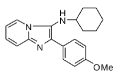
Our implementation is first validated by comparison against TD-DFT calculations with the GTO-based program deMon2k for the historically-important test case of N2 JCS96 ; CJC+98 . This allows us to see and discuss some of the pros and cons of wavelets versus GTOs. We then go on to apply the method to a real-world application, namely the calculation of the absorption spectrum of a molecule of potential interest as a fluorescent probe in biological applications. This molecule, -cyclohexyl-2-(4-methoxyphenyl)imidazo[1,2-]pyridin-3-amine (Fig. 1), will simply be referred to as Flugi 6 BMO11 . Since this molecule has not been thoroughly characterized before we have included an experimental section describing our determination of its x-ray crystal structure.
This paper is organized as follows: The basic equations of TD-DFT are reviewed in the next section. In Sec. III, we briefly review the idea of wavelets, explain how we handle the integral evaluation in our implementation of TD-DFT, and Section IV discuss the pros and cons of the wavelet implementation in the context of N2 calculations with BigDFT and the GTO-based code deMon2k. Section V reports the x-ray crystal structure, and experimental and calculated UV/visible absorption spectrum of Flugi 6. An assignment is also made of the peaks appearing in the spectrum. The final section contains our concluding discussion.
II Time-Dependent Density-Functional Theory
As evidenced by the numerous review articles GK90 ; GUG94 ; C95 ; GDP96 ; C96 ; BG98 ; L01 ; VBB+01 ; C02 ; D03 ; MG03 ; MG04 ; BWG05 ; DH05 ; CMA+06 ; C08 ; C09 ; CH12 and books MS90 ; MUN+06 ; GMNR11 written on the subject, TD-DFT is now such a well-established formalism that little additional review seems necessary. Nevertheless the purpose of this section is to recall a few key equations in order to keep the present paper reasonably self-contained and to introduce notation.
Time-dependent DFT builds upon the Kohn-Sham formulation of ground-state DFT KS65 . In its modern formulation, Kohn-Sham DFT is spin-DFT so that the total energy involves an exchange-correlation (xc) energy which depends upon the density of spin- electrons and the density of spin- electrons. These are obtained as the sum of the densities of the occupied orbitals of each spin,
| (1) |
where is the occupation number of orbital and, the total charge density is given as the sum of the charge densities of two spin components. The Kohn-Sham orbitals are obtained by solving the Kohn-Sham equation,
| (2) |
This involves a single-particle potential,
| (3) |
which is the sum of the external potential (i.e., the interaction of the electrons with the nuclei and any applied electronic fields), the Hartree potential,
| (4) |
which may alternatively be obtained as the solution of Poisson’s equation,
| (5) |
and the xc-potential which is just the functional derivative of the xc-energy,
| (6) |
Together and constitute the self-consistent field (SCF), . Modern DFT often uses a type of generalized Kohn-Sham formalism where the SCF may contain some orbital dependence due to (say) inclusion of some fraction of Hartree-Fock exchange and the external potential may even include a nonlocal part. In particular this latter generalization is the case when nonlocal pseudopotentials are employed, as is the case in BigDFT.
The external potential is time-dependent in TD-DFT, and the time-dependent Kohn-Sham potential has the form,
| (7) |
where the external potential,
| (8) |
The dependence of the xc part on the initial interacting () and noninteracting () wave functions may be eliminated by using the first Hohenberg-Kohn theorem HK64 if the initial state is the ground stationary state. This is case when seeking the linear response of the ground stationary state to an applied electronic field. The TD charge density,
| (9) |
then suffices to calculate the induced dipole moment (at least for finite systems such as molecules) and hence the dynamic polarizability,
| (10) |
whose poles give the excitation energies of the system,
| (11) |
and whose residues give the corresponding oscillator strengths,
| (12) |
The excitation energies and oscillator strengths are often presented in the form of a stick spectrum consisting of lines of height located at the associated . What is actually measured is the molar extinction coefficient , in Beer’s law. To a first approximation, this is related to the spectral function,
| (13) |
by,
| (14) |
in SI units H82 ; H83 ; H02 . Finite spectrometer resolution, vibrational, and solvent effects are traditionally approximated by replacing the Dirac delta functions in Eq. (13) with a Gaussian whose full-width at half-maximum (FWHM) is selected to match the experimental spectrum and we will do the same. Solvent effects may also shift excitation energies BM54a ; BM54b ; L57 ; LP57 ; M57 ; B64 ; BSK76 and affect oscillator strengths C34 ; MR41 ; W64 ; L66 ; BW68 ; A70 ; MB80 ; AI86 ; A91 ; HB94 ; BGK06 . While these effects are not necessarily small (vide infra), we will simply ignore them when comparing with experimental data as this is a reasonable first approximation.
Practical TD-DFT calculations typically make use of the TD-DFT adiabatic approximation,
| (15) |
because even less is known about the exact xc-potential in TD-DFT than is the case for regular DFT. Here is regarded at fixed as a function of . If in addition, the xc-energy functional is of the local density approximation (LDA) or generalized gradient approximation (GGA) type, the TD-DFT adiabatic approximation is typically found to work well for low-energy excitations of dominant one-hole/one-particle character which are not too delocalized in space and do not involve too much charge transfer. Several extensions of classic TD-DFT have been found to be useful for going beyond these restrictions (see for example Ref. C09 ; CH12 for a review).
One of us used a density-matrix formalism to develop a random-phase approximation (RPA) like formalism for the calculation of absorption spectra from the dynamic polarizability [Eq. (10)] C95 . This allowed the calculation of TD-DFT spectra to be quickly implemented in a wide variety of quantum chemistry programs since most of the available computational framework was already in place. The precise equation that needs to be solved is, within the TD-DFT adiabatic approximation,
| (16) |
Here,
| (17) |
and the coupling matrix is given by,
| (18) |
where we are making use of the index convention that orbitals are unoccupied, orbitals are occupied, and orbitals are free to be either occupied or unoccupied. In the case of an LDA or GGA, Eq. (16) may be rearranged to give the lower-dimensional matrix equation,
| (19) |
where
| (20) |
Alternatively the Tamm-Dancoff approximation (TDA) is sometimes found to be useful HH99 ,
| (21) |
This is particularly the case when it is necessary to attenuate the effect of spin-instabilities on potential energy surfaces when investigating photoprocesses CND11 .
III Implementation in BigDFT
Our implementation of the equations of the previous section in BigDFT is described in this section and their validation by comparison against calculations with deMon2k is described in the next section.
BigDFT solves the Kohn-Sham equation [Eq. (2)] in the pseudopotential approximation. The main difference is that the external potential part, , of the Kohn-Sham potential, , is manipulated so as to smooth the behavior of the Kohn-Sham orbitals in the core region near the nuclei while preserving the form of the Kohn-Sham orbitals outside the core region. This is done through the use of Goedecker-Teter-Hutter (GTH) pseudopotentials GTH96 in order to avoid “wasting” wavelets on describing the nuclear cusp. These include both a local and nonlocal part and are used for all atoms (even hydrogen). Several different functionals are available for the xc-energy. However we will only be considering the LDA functional with Teter’s Pade approximation GTH96 of Ceperley and Alder’s quantum Monte Carlo results CA80 since the xc-kernel, , is thus far only implemented in BigDFT at the LDA level.
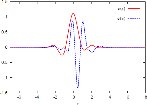
There are two fundamental functions in Daubechies family: the scaling function and the wavelet (see Fig. 7.) Note that both types of function are localized with compact support. The full basis set can be obtained from all translations by a certain grid spacing h of the scaling and wavelet functions centered at the origin. These functions satisfy the fundamental defining equations,
| (22) |
which relate the basis functions on a grid with spacing and another one with spacing . The coefficients, hj and gj, consitute the so-called “filters” which define the wavelet family of order . These coefficients satisfy the relations, and . Equation (39) is very important since it means that a scaling-function basis defined over a fine grid of spacing may be replaced by combining a scaling-function basis over a coarse grid of spacing with a wavelet basis defined over the fine grid of spacing . This then gives us the liberty to begin with a coarse description in terms of scaling functions and then add wavelets only where a more refined description is needed. In principle the refined wavelet description may be further refined by adding higher-order wavelets where needed. However in BigDFT we restricted ourselves to just two levels: coarse and fine associated respectively with scaling functions and wavelets.
For a three-dimensional description, the simplest basis set is obtained by a tensor product of one-dimensional basis functions. For a two resolution level description, the coarse degrees of freedom are expanded by a single three dimensional function, , while the fine degrees of freedom can be expressed by adding another seven basis functions, , which include tensor products with one-dimensional wavelet functions.
Thus, the Kohn-Sham wave function is of the form
| (23) |
The sum over i1,i2,i3 runs over all the grid points contained in the low-resolution regions and the sum over j1,j2,j3 runs over all the points contained in the (generally smaller) high resolution regions. Each wave function is then described by a set of coefficients . Only the nonzero scaling function and wavelet coefficients are stored. The data is thus compressed. The basis set being orthogonal, several operations such as scalar products among different orbitals and between orbitals and the projectors of the nonlocal pseudopotential can be directly carried out in this compressed form. In addition to raw Daubechies scaling functions, practical applications make use of autocorrelated functions to make interpolating scaling functions (ISF) DD89 . In particular, as shown by A. Neelov and S. Goedecker NG+06 , the local potential matrix elements approximated using the linear combination of such ISFs is exact for polynomial expansions up to 7th order and the corresponding Kohn-Sham densities can be calculated by the real-valued coefficients on the grid points.
Although not every grid point is associated with a basis function and the fine grid is only used in some regions of space, the Daubechies basis set is still very large. This means that full diagonalization of the Kohn-Sham orbital Hamiltonian is not possible. Instead the direct minimisation method D75 ; MRD91 is used to obtain the occupied orbitals. This is in contrast with the GTO-based deMon2k program which will be described below in which full diagonalization of the Kohn-Sham orbital Hamiltonian matrix is carried out within the finite GTO basis set.
A key point to review because of its importance for our implementation of TD-DFT in BigDFT is the Poisson solver used to treat the Hartree part of the potential, . Although this Poisson solver has been discussed elsewhere GDN+06 ; GDG07 , we briefly review how it works in order to keep this article somewhat self-contained. The Hartree potential is evaluated as,
| (24) |
where is the Green’s function for the Poisson equation, namely just the Coulomb potential. The density and potential are expanded in a set of interpolating scaling functions,
| (25) |
associated with the same grid of points, , in real space. In particular, the charge density coefficients, . Then,
| (26) |
where the quantity,
| (27) |
is translationally invariant by construction. Since Eq. (43) has the form of a three dimensional convolution, it may be efficiently evaluated by using appropriate parallelized fast Fourier transform algorithms at the cost of only operations. The calculation of matrix elements of the Green’s function is simplified by using a separable approximation in terms of Gaussians,
| (28) |
so that all the complicated 3-dimensional integrals are reduced to products of simpler 1-dimensional integrals. For more information about BigDFT, the reader is referred to the program website bigdft and to various publications GDN+06 ; GDG07 ; GNG+08 ; AGGNG09 ; GODMNG09 ; GVO+11 .
We are now in a position to understand the construction of the coupling matrix in our implementation of TD-DFT in BigDFT, which we split into the Hartree and exchange-correlation parts,
| (29) |
Instead of calculating the Hartree part of coupling matrix directly as,
| (30) |
we express the coupling matrix element as,
| (31) |
where,
| (32) |
and,
| (33) |
The advantage of doing this is that, although and are neither real physical charge densities nor real physical potentials, they still satisfy the Poisson equation,
| (34) |
and we can make use of whichever of the efficient wavelet-based Poisson solvers already available in BigDFT, is appropriate for the boundary conditions of our physical problem.
Once the solution of Poisson’s equation, , is known, we can then calculate the Hartree part of the kernel according to Eq. (48). Inclusion of the exchange-correlation kernel is accomplished by evaluating,
| (35) |
where,
| (36) |
We note that for the LDA, so that no integral need actually be carried out in evaluating . The integral in Eq. (52) is, of course, carried out numerically in practice as a discrete.
IV Validation
Having implemented TD-DFT in BigDFT we now desire to validate our implementation by testing it against another program in which TD-DFT is already implemented, namely the all-electron GTO-based program deMon2k deMon2k . deMon2k resembles a typical GTO-based quantum chemistry program in that all the integrals other than the xc-integrals, can be evaluated analytically. In particular, deMon2k has the important advantage that it accepts the popular GTO basis sets common in quantum chemistry and so can benefit from the experience in basis set construction of a large community built up over the past 50 years or so. In the following, we have chosen to use the well-known correlation-consistent basis sets for this study F96 ; SDESGCW07 . (Note, however, that the correlation-consistent basis sets used in deMon2k lack and functions but are otherwise exactly the same as the usual ones.) The advantage of using these particular basis sets is that there is a clear hierarchy as to quality.
An exception to the rule that integrals are evaluated analytically in deMon2k are the xc-integrals (for the xc-energy, xc-potential, and xc-kernel) which are evaluated numerically over a Becke atom-centered grid. This is important because the relative simplicity of evaluating integrals over a grid has allowed the rapid implemenation of new functionals as they were introduced. We made use of the fine fixed grid in our calculations.
As described so far, deMon2k should have scaling because of the need to evaluate 4-center integrals. Instead deMon2k uses a second atom-centered auxiliary GTO basis to expand the charge density. This allows the the elimination of all 4-center integrals so that only 3-center integrals remain for a formal scaling. In practice, integral prescreening leads to scaling where is typically between 2 and 3. We made use of the A3 auxiliary basis set from the deMon2k automated auxiliary basis set library.
All calculations were performed using standard deMon2k default criteria. Although full TD-LDA calculations are possible with deMon2k, the TD-LDA calculations reported here all made use of the TDA. The chosen test molecule was N2 with an optimized bond length of 1.115 Å. This molecule was chosen partly because of its small size but also because of the large number of excited states which are well characterized (see Refs. JCS96 ; CJC+98 and references therein.)
Unlike TD Hartree-Fock (or configuration interaction singles) calculations, TD-LDA calculations are preprepared to describe excitation processes in the sense that the occupied and unoccupied orbitals both see the same number of electrons (because they come from the same local potential). This means that there is often little relaxation — at least in small molecules — and a two orbital model C95 ; C08 ; CH12 ; CGG+00 often provides a good first approximation to the singlet () and triplet () excitation energies,
| (37) |
Consideration of typical integral signs and magnitudes then implies that
| (38) |
with the singlet-triplet splitting going to zero for Rydberg states (in which case the electron repulsion integrals become negligible due to the diffuse nature of the target orbital .)
| Basis Set | |||
|---|---|---|---|
| STO-3G | 7.6758 | 0.0297 | 7.6461 |
| DZVP | 10.1824 | 2.2616 | 7.9208 |
| TZVP | 10.2142 | 2.2894 | 7.9248 |
| CC-PVDZ | 9.8656 | 1.8993 | 7.9663 |
| CC-PVTZ | 10.2978 | 2.2868 | 8.0110 |
| CC-PVQZ | 10.3545 | 2.3527 | 8.0018 |
| CC-PV5Z | 10.3786 | 2.3886 | 7.9900 |
| CC-PCVDZ | 9.9197 | 1.9314 | 7.9883 |
| CC-PCVQZ | 10.3555 | 2.3532 | 8.0023 |
| CC-PCVTZ | 10.2372 | 2.2718 | 8.0154 |
| CC-PCV5Z | 10.3793 | 2.3891 | 7.9902 |
| AUG-CC-PVDZ | 10.3534 | 2.3785 | 7.9749 |
| AUG-CC-PVQZ | 10.3987 | 2.4127 | 7.9860 |
| AUG-CC-PVTZ | 10.3953 | 2.4010 | 7.9943 |
| AUG-CC-PV5Z | 10.3984 | 2.4137 | 7.9847 |
| AUG-CC-PCVDZ | 10.3732 | 2.3879 | 7.9847 |
| AUG-CC-PCVTZ | 10.3972 | 2.4015 | 7.9957 |
| AUG-CC-PCVQZ | 10.3990 | 2.4124 | 7.9866 |
| AUG-CC-PCV5Z | 10.3985 | 2.4136 | 7.9849 |
| hg111 Grid spacing of the cartesian grid in atomic units./m222 Coarse grid multiplier (crmult) /n333Fine grid multiplier (frmult) | |||
|---|---|---|---|
| Low resolution | |||
| 0.4/6/8 | 10.3910 | 2.3815 | 8.0095 |
| 0.4/7/8 | 10.3964 | 2.3922 | 8.0042 |
| 0.4/8/8 | 10.3971 | 2.3945 | 8.0027 |
| 0.4/9/8 | 10.3972 | 2.3951 | 8.0022 |
| 0.4/10/8 | 10.3973 | 2.3953 | 8.0020 |
| 0.4/11/8 | 10.3972 | 2.3953 | 8.0019 |
| High resolution | |||
| 0.3/7/8 | 10.3977 | 2.3932 | 8.0043 |
| 0.3/8/8 | 10.3984 | 2.3957 | 8.0027 |
| 0.3/9/8 | 10.3985 | 2.3963 | 8.0022 |
| 0.3/10/8 | 10.3985 | 2.3965 | 8.0021 |
| 0.3/11/8 | 10.3985 | 2.3965 | 8.0020 |
Since orbital energy differences provide an important first estimate of TD-DFT excitation energies, we wished to see how rapidly they converged for BigDFT and deMon2k as the quality of the basis set was improved. Tables 1 and 2 show how the highest occupied molecular orbital (HOMO) – lowest unoccupied molecular orbital (LUMO) energy gap () varies for each program.
Consider first how deMon2k calculations of evolve as the basis set is improved (Table 1). Jamorski, Casida, and Salahub had earlier shown that LUMO is bound for reasonable basis sets JCS96 . (Small differences between the present calculations and those in Ref. JCS96 are due to gradual improvements in the grid, auxiliary basis sets, and convergence criteria used in the deMon programs). Convergence to the true HOMO-LUMO LDA gap is expected with systematic improvement within the series: (i) double zeta plus valence polarization (DZVP) triple zeta plus valence polarization (TZVP), (ii) augmented correlation-consistent double zeta plus polarization plus diffuse on all atoms (AUG-CC-PCVDZ) AUG-CC-PCVTZ (triple zeta) AUG-CC-PCVQZ (quadruple zeta) AUG-CC-PCV5Z (quintuple zeta), (iii) augmented correlation-consistent valence double zeta plus polarization plus diffuse (AUG-CC-PVDZ) AUG-CC-PVTZ AUG-CC-PVQZ AUG-CC-PV5Z, (iv) correlation-consistent double zeta plus polarization plus tight core (CC-PCVDZ) CC-PCVTZ CC-PCVQZ CC-PCV5Z, and (v) correlation-consistent valence double zeta plus polarization on all atoms (CC-PVDZ) CC-PVTZ CC-PVQZ CC-PV5Z. There is a clear tendency in the correlation-consistent basis sets to tend towards values of 10.40 eV for the HOMO energy, 2.42 eV for the LUMO energy, and 8.01 eV for , with adequate convergance already achieved with the CC-PVTZ basis set.
Now let us turn to BigDFT (Table 2). Calculations were done for two different grid values, denoted by hg = 0.3, 0.4. (These values are the nodes of the grid in atomic units which serve as centers for the scaling function/wavelet basis.) The simulation “box” has the shape of the molecule and its size is expressed in the units of the coarse grid multiplier (crmult) and the fine grid multiplier (frmult) which determines the radius for the low/high resolution sphere around the atom. Results using 16 unoccopied orbitals with the different wavelet basis sets are essentially identical, with no significant variation in the HOMO energy, the LUMO energy, and the value of 8.00 eV between the high resolution combination of 0.3/11/8 and the low resolution combination of 0.4/6/8.
The remaining differences for the HOMO energy, LUMO energy, and calculated by the two programs, deMon2k and BigDFT, is more difficult to trace. For example, it might be due to the auxiliary basis approximation in deMon2k or to the use of pseudopotentials in BigDFT or perhaps to still other program differences. The important point is that differences are remarkably small.
| State | BigDFT111Present work (TD-LDA/TDA). | deMon2k222Present work (TD-LDA/TDA). | ABINIT333From abinit-tddft (TD-LDA). | Experiment444Taken from Ref.(BK90 ). |
|---|---|---|---|---|
| 1 | 10.71 | 10.39 | 9.16 | 12.0 |
| 1 | 10.58 | 10.38 | 10.79 | 11.19 |
| 1 | 10.29 | 9.99 | 10.46 | 10.27 |
| 1 | 9.37 | 9.36 | 9.92 | 9.92 |
| 1 | 9.36 | 9.36 | 9.91 | 9.67 |
| 1 | 9.35 | 9.10 | 9.47 | 9.31 |
| 1 | 8.93 | 8.60 | 9.08 | 8.88 |
| 1 | 7.69 | 7.83 | 7.85 | 7.75 |
| 1 | 8.52 | 8.43 | 8.16 | 8.04 |
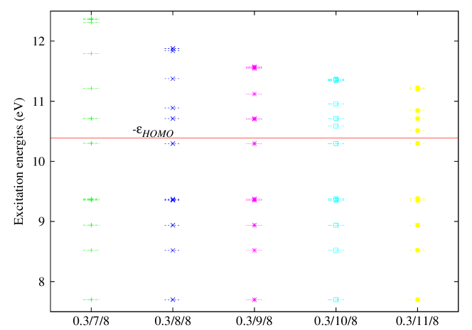
We now come to the calculation of the actual excited states of N2 and the third reason alluded to in the introduction that quantum chemists have been slow to adapt grid-based methods. This is the concern that the very large size of basis sets in grid-based methods would lead to impractically-large configuration interaction expansions. Put differently, this concerns the basic problem of how to handle the continuum. A correct inclusion of the continuum in the formalism of Sec. II would seem to require at least approximate integrals over a quasicontinuum of unoccupied orbitals. Clearly this is impractical and our method only uses the first several unoccupied orbitals. This is perhaps reasonable for the lower excited states, given the anticipated dominance of the two-orbital model [Eq. (37)], but may fail to be quantitative when relaxation or state mixing starts to become important and the two-orbital model breaks down. This problem is avoided in quantum chemistry where the virtual orbitals in the TD-DFT calculation have an altogether different meaning: they are simply there to describe the dynamic polarizability of the ground-state charge density and need not describe the continuum well. This is why fewer unoccupied orbitals are normally needed in quantum chemical applications of TD-DFT than is the case when using, say, plane waves. In Fig. 3 the lowest few excited-states are calculated using BigDFT. This figure shows that the excited states calculated with different grids are essentially the same up to -. After -, increasing the quality of the basis set by varying the simulation box sizes leads to an increasing collapse of the higher excited-states. This is a reflection of the fact that the TD-LDA ionization continuum starts at - which is about 5 eV low because of the incorrect asymptotic behavior of the xc-potential CJC+98 . Of course, as indicated by the estimate (37), the excitation energy is not exactly a simple orbital energy difference, but they are closely related.
With these caveats, let us see how well our implementation of TD-DFT does in BigDFT. Table 3, lists the lowest nine excited states of N2 calculated with deMon2k and BigDFT. For comparison, Table 3 also contains full TD-LDA (i.e, non-TDA) excitation energies obtained from ABINIT abinit using the Perdew-Wang 92 parameterisation of the LDA functional PW92 along with the experimental values from the literature BK90 . The slight differences which occur between the 1 and 1 excitation energies in the BigDFT and ABINIT calculations are an indication of residual numerical errors since these two states are rigorously degenerate by symmetry when using the TD-LDA and TD-LDA/TDA approximations: Aside from this tiny difference, it is certainly reassuring that excitation energies calculated with BigDFT, deMon2k, and ABINIT are quite similar. Nevertheless differences as large as 0.3 eV or more are found for some states. Such differences are large enough to be potentially problematic for determining the ordering of near-lying states.

Finally since a large number of excited states have been calculated, it is interesting to test the assertion that the oscillator strength distribution should be approximately correct even above the TD-LDA ionization threshold at - CJC+98 . This is especially true since the transitions given in Table 3 are all dark and we would like to see how the oscillator strengths of bright states compare. The high-energy spectra are compared in Fig. 4 using Eq. (14). Clearly the spectra are in reasonable qualitative agreement.
The above results show that this first implementation of BigDFT is quantitative — especially when results are dominated by bound-bound transitions — and our discussion may eventually suggest ways to go further towards improving the method. In the meantime, we have a method that can be used for moderate-size molecules and this is illustrated in the next section.
V Application
A large series of fluorescent molecules of potential interest as biological markers GR03 has recently been synthesized by combinatorial chemistry BMO11 . This is a method whereby large sets of similar reactions are conducted in parallel in arrays of spots on a single plate, thus dramatically increasing throughput when searching for molecules with a particular property — in this case fluorescence. We have chosen to calculate the absorption spectrum of one of these fluorescent molecules in preparation for future more in-depth theoretical studies of their fluorescence properties using BigDFT. This molecule, which we will simply refer to as Flugi 6 (because it is molecule 6 BMO11 among the fluorescent molecules prepared by the UGI reaction u62 ) rather than by its full name of -cyclohexyl-2-(4-methoxyphenyl)imidazo[1,2-]pyridin-3-amine is shown in Fig. 1. The synthesis and partial characterization of Flugi 6 has been described in Ref. BMO11 . However we go further here and report the experimental determination of its crystal structure. We then go on to compare the spectrum calculated with BigDFT with the measured spectrum and discuss the problem of peak assignment.
V.1 X-ray Crystal Structure
Crystals of Flugi 6 (C20H23N3O, = 321.42 g/mol) were obtained out of recrystallisation in ethyl acetate (EtOAc) as colorless needles suitable for X-ray diffraction. A 0.38 mm 0.28 mm 0.01 mm crystal was mounted on a glass fiber using grease and centered on a Bruker Enraf Nonius kappa charge-coupled device (CCD) detector working at 200 K and at the monochromated (graphite) Mo Kα radiation = 0.71073 Å. The crystal was found to be orthorhombic, Pna21, = 27.912(4) Å , = 5.876(2)Å, = 10.297(2) Å, = 1688.7(6) Å3, = 4, = 1.264 g.cm-3, = 0.080 mm-1. A total of 17700 reflections were collected using and scans; 2853 independent reflections ( = 0.1557). The data were corrected for the Lorentz and polarization effects. The structure was solved by direct methods with SIR92 ACGG93 and refined against F by leastsquare method implemented by TeXsan TeXsan . C, N, and O atoms were refined anisotropically by the full matrix least-squares method. H atoms were set geometrically and recalculated before the last refinement cycle. The final values for 1964 reflections with (I) and 217 parameters are = 0.0617, = 0.0657, goodness of fit (GOF) = 1.78 and for all 2854 unique reflections = 0.0923 , = 0.0829, GOF = 1.85. The resultant crystal geometry is given in 4
| Atom | |||
|---|---|---|---|
| O | 14.0340 | 1.5882 | 2.9552 |
| N | 7.7362 | 0.5932 | 7.4268 |
| N | 9.1303 | 2.5361 | 7.6402 |
| N | 8.7184 | -0.6003 | 5.8202 |
| C | 8.8581 | 1.3112 | 7.0430 |
| C | 7.6978 | -0.5625 | 6.6613 |
| C | 6.7910 | 0.8587 | 8.3836 |
| C | 5.8275 | -0.0445 | 8.6210 |
| C | 9.4459 | 0.5452 | 6.0467 |
| C | 12.4814 | 2.2280 | 4.5690 |
| C | 9.6943 | 2.5959 | 8.9709 |
| C | 12.2450 | 0.0746 | 3.5887 |
| C | 12.9311 | 1.2651 | 3.6923 |
| C | 11.3663 | 2.0047 | 5.3306 |
| C | 11.1149 | -0.1284 | 4.3608 |
| C | 10.6426 | 0.8232 | 5.2590 |
| C | 5.7504 | -1.2331 | 7.8594 |
| C | 6.6706 | -1.4857 | 6.8881 |
| C | 11.0628 | 2.0293 | 9.0805 |
| C | 14.5914 | 0.5796 | 2.1251 |
| C | 9.6456 | 4.0228 | 9.4571 |
| C | 10.1882 | 4.1778 | 10.8473 |
| C | 11.6027 | 2.1400 | 10.5019 |
| C | 11.5598 | 3.5428 | 10.9936 |
| H | 6.8178 | 1.6727 | 8.8752 |
| H | 5.1910 | 0.1163 | 9.3101 |
| H | 12.9482 | 3.0519 | 4.6478 |
| H | 9.1307 | 2.0846 | 9.5420 |
| H | 12.5454 | -0.6011 | 2.9948 |
| H | 11.0776 | 2.6830 | 5.9322 |
| H | 10.6436 | -0.9486 | 4.2766 |
| H | 5.0541 | -1.8576 | 8.0282 |
| H | 6.6161 | -2.2802 | 6.3725 |
| H | 11.0384 | 1.1132 | 8.8327 |
| H | 11.6406 | 2.5025 | 8.4958 |
| H | 10.1595 | 4.5627 | 8.8705 |
| H | 8.7422 | 4.3165 | 9.4511 |
| H | 10.2551 | 5.1036 | 11.0519 |
| H | 9.5907 | 3.7627 | 11.4607 |
| H | 11.0761 | 1.5956 | 11.0779 |
| H | 12.5025 | 1.8356 | 10.5174 |
| H | 12.1865 | 4.0570 | 10.5007 |
| H | 11.8007 | 3.5496 | 11.9149 |
| H | 15.3192 | 0.9409 | 1.6353 |
| H | 14.8996 | -0.1395 | 2.6665 |
| H | 13.9283 | 0.2626 | 1.5256 |
| H | 8.9445 | 3.3408 | 7.1731 |
The data have been deposited with the Cambridge Crystallographic Data Centre (Reference No. CCDC 8200007). This material is available free of charge via www.ccdc.can.ac.uk/conts/retrieving.html (or from the Cambridge Crystallographic Data Centre, 12 Union Road, Cambridge CB2 1EZ, UK. Fax: +44-1223-336033. E-mail: deposit@ccdc.cam.ac.uk).
V.2 Spectrum
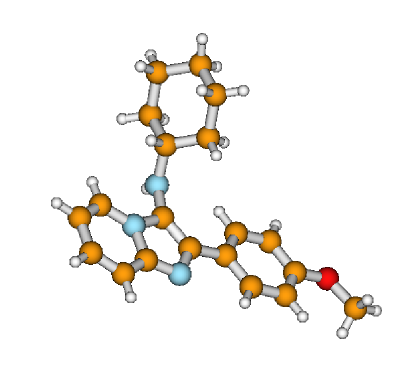
The experimental UV/Vis spectrum was determined in dimethyl sulphur dioxide (DMSO) as described in the supplementary material of Ref. BMO11 The first step to calculating the spectrum of Flugi 6 is to optimize the geometry. This was done with BigDFT using the 0.4/8/8 grid, beginning with the experimental crystal geometry shown in Fig. 5. Our optimized geometry is given in Table 5. The largest change 0.15 Å from the initial guess is for the 18th atom of hydrogen. It was verified that the optimized geometry is indeed a minimum by explicit calculation of vibrational frequencies. However the experimental geometry is not identical to our calculated gas phase geometry as confirmed by the presence of three imaginary vibrational frequencies calculated for the (unoptimized) experimental geometry.
| Atom | |||
|---|---|---|---|
| O | 14.0374 | 1.5760 | 2.9779 |
| N | 7.75774 | 0.5820 | 7.4296 |
| N | 9.14347 | 2.5138 | 7.6339 |
| N | 8.73705 | -0.581 | 5.7976 |
| C | 8.85269 | 1.3197 | 7.0273 |
| C | 7.73253 | -0.574 | 6.6557 |
| C | 6.82855 | 0.8581 | 8.3749 |
| C | 5.83564 | -0.044 | 8.6043 |
| C | 9.44155 | 0.5586 | 6.0148 |
| C | 12.4807 | 2.2541 | 4.5863 |
| C | 9.66483 | 2.5868 | 8.9771 |
| C | 12.2472 | 0.0755 | 3.6050 |
| C | 12.9348 | 1.2789 | 3.7031 |
| C | 11.3530 | 2.0325 | 5.3457 |
| C | 11.1111 | -0.130 | 4.3645 |
| C | 10.6388 | 0.8366 | 5.2444 |
| C | 5.77383 | -1.232 | 7.8551 |
| C | 6.70657 | -1.492 | 6.8869 |
| C | 11.0671 | 2.0245 | 9.0831 |
| C | 14.5517 | 0.5791 | 2.1429 |
| C | 9.63546 | 4.0197 | 9.4485 |
| C | 10.1799 | 4.1615 | 10.852 |
| C | 11.5902 | 2.1260 | 10.497 |
| C | 11.5622 | 3.5584 | 10.985 |
| H | 6.94062 | 1.8172 | 8.8855 |
| H | 5.08962 | 0.1718 | 9.3696 |
| H | 13.0361 | 3.1924 | 4.6593 |
| H | 9.01856 | 1.9925 | 9.6670 |
| H | 12.5948 | -0.707 | 2.9284 |
| H | 11.0089 | 2.7962 | 6.0486 |
| H | 10.5470 | -1.064 | 4.2928 |
| H | 4.97202 | -1.948 | 8.0454 |
| H | 6.68074 | -2.397 | 6.2775 |
| H | 11.0746 | 0.9834 | 8.7183 |
| H | 11.7169 | 2.5999 | 8.3962 |
| H | 10.2520 | 4.6168 | 8.7465 |
| H | 8.60472 | 4.4110 | 9.3825 |
| H | 10.1918 | 5.2227 | 11.149 |
| H | 9.49548 | 3.6524 | 11.557 |
| H | 10.9656 | 1.5016 | 11.164 |
| H | 12.6112 | 1.7164 | 10.558 |
| H | 12.2802 | 4.1561 | 10.392 |
| H | 11.9013 | 3.6190 | 12.032 |
| H | 15.4016 | 1.0289 | 1.6155 |
| H | 14.9021 | -0.292 | 2.7251 |
| H | 13.8030 | 0.2392 | 1.4055 |
| H | 8.94041 | 3.3910 | 7.1600 |
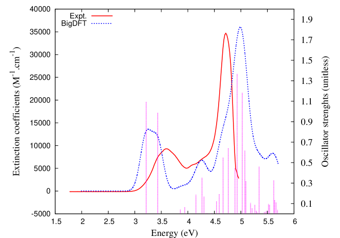
The TD-LDA absorption spectrum of Flugi 6 was then calculated at the optimized geometry using our new implementation of TD-DFT in BigDFT. In addition to the previously mentioned computational details, the calculation used 60 unoccupied orbitals within the TDA. The excited-states were obtained using full-matrix diagonalization of the TD-DFT part. The theoretical spectrum was calculated using Eq. (14) using a FWHM of 0.25 eV and then transformed to a wavelength scale using our spectrum convolution program pablo . Because we were restricted to a more limited number of unoccupied orbitals than in the N2 test case, there is some concern that our calculated spectrum might change if a larger number of unoccupied orbitals is included. However the comparison of the theoretical and experimental results shown in Fig. 6 is reasonable. This is especially true when it is kept in mind that we are comparing gas-phase theory with an experimental spectrum measured in a polar solvent DMSO. Notice the presence of a larger peak at 4.6-5.0 eV, a smaller peak at 3.2-3.5 eV, and a shoulder inbetween near 4.3 eV.
| Dominant transition111 and stand respectively for HOMO and LUMO. | Coefficient222Configuration interaction (CI) expansion coefficient. | ||
|---|---|---|---|
| 4.83006 | 0.047 | 0.698419 | |
| 4.81870 | 0.890 | 0.402878 | |
| 4.77478 | 0.054 | 0.662945 | |
| 4.72164 | 0.373 | 0.423823 | |
| 4.63424 | 0.665 | 0.308510 | |
| 4.58075 | 0.572 | 0.279673 | |
| 4.50552 | 0.048 | 0.654877 | |
| 4.47587 | 0.012 | 0.396204 | |
| 4.38722 | 0.037 | 0.496849 | |
| 4.33889 | 0.005 | 0.550260 | |
| 4.29785 | 0.007 | 0.332720 | |
| 4.24700 | 0.221 | 0.418216 | |
| 4.12777 | 0.495 | 0.358160 | |
| 3.92056 | 0.116 | 0.431698 | |
| 3.78973 | 0.042 | 0.418160 | |
| 3.50331 | 0.883 | 0.523227 | |
| 3.21284 | 1.386 | 0.615044 |
In contrast to experience with ruthenium complexes (to name but one example), Eq.(14) with gaussian broadening does not suffice in the present case to give good agreement between theoretical and experimental molar extinction coefficinets. This is why the theoretical curve has been divided magnitude by a factor of ten. We believe that this discrepancy is in part due to the aforementioned solvent effects on excitation energies and oscillator strengths which we have chosen to neglect and in part due to the possible presence of multiple conformers in the room temperature experiment. This latter hypothesis might be tested by expensive dynamics calculations, but this far beyond the scope of the present work. Nevertheless, even without dynamics we find this level of agreement to be encouraging and now go on to further analyze our calculated spectrum. The calculated stick spectrum is also shown in Fig. 6. It is now clear that the small peak at 3.2-3.5 eV corresponds to two transitions, that the shoulder near 4.3 eV corresponds to three transitions, and that the large peak at 4.6-5.0 eV corresponds to several electric excited states. Table 6 provides a more detailed analysis. All of the transitions are below the onset of TD-LDA ionization continuum at = 4.8713 eV, which is artificially low compared to the true ionization energy CJC+98 . As mentioned in Sec. III, unlike TD Hartree-Fock (or configuration interaction singles) calculations, TD-LDA calculations are preprepared to describe excitation processes in the sense that the occupied and unoccupied orbitals both see the same number of electrons (because they come from the same local potential.) This means that there is often little relaxation — at least in small molecules — and a two orbital model C95 provides a good first approximation to the excitation energy [Eqs. (37) and (38)]. The TDA configuration interaction coefficient is then determined by spin coupling and is given by . Table 6 shows significant deviations from this theoretical value, suggesting significant relaxation effects may be taking place. Visualization of the HOMO and LUMO suggests that relaxation is important here and might help to explain why the first peak is at slightly too low an energy compared to the first experimental peak in the absorption spectrum CGG+00 . Nevertheless, the energy of HOMO LUMO dominated singlet transition at 3.21 eV exceeds the simple difference of HOMO and LUMO molecular orbital energies of 2.80 eV as expected from the domination of the Hartree term over the two xc terms. Two interesting features, which will not be pursued in the present paper, are the absence of oscillator strength for the transition and the indication of significant configuration mixing for the first and seventh transitions which both borrow from and for the third and fifth transitions which both borrow from .
VI Conclusion
Grid-based methods have long been regarded with skepticism by the quantum chemistry community, but have now been accepted in the form of the grids used to evaluate xc-integrals in the DFT part of most quantum chemistry codes. We believe that an even greater acceptance of grid-based methods may prove useful as theoretical solid-state and chemical physics strive to meet on “neutral ground” at the nanometer scale. Acceptance will be aided by continuing advances in grid-based methods with wavelets being of particular interest here. At the same time, new features should be added to grid-based electronic structure codes in order to make them more useful for chemical applications. This paper represents a small step in that direction. In particular, we have presented the first implementation of TD-DFT in a wavelet-based code, namely in BigDFT.
While BigDFT is designed for routine calculations on systems containing many hundreds of atoms, this first implementation of TD-DFT in BigDFT is not yet ready for these more ambitious applications. Rather, we wished to bring out the pros and cons of wavelet-based TD-DFT by comparing against a GTO-based quantum chemistry code (in this case, deMon2k) and by an example application showing how our implementation in BigDFT can be useful in analyzing the spectrum of a molecule of contemporary experimental interest.
A factor in favor of the wavelet-based approach is the rapidity of convergence of the bound orbitals and orbital energies with respect to refinements of the wavelet basis and associated grid. While orbital results from the all-electron deMon2k code are not (and should not) be in exact agreement with those of the pseudopotential BigDFT code, the results are really quite close when sufficiently large basis sets are used. In the case of the GTO-based code, tight basis set convergence typically requires going beyond at least the triple-zeta-valence-plus-polarization (TZVP) level. In contrast, adequate orbital convergence is easily obtained with BigDFT using the default wavelet basis set and grid, with further refinements leading to only minor improvement. This comes close to the quantum chemists’ dream of calculations free of errors due to basis set incompleteness.
Interestingly, problems which could be envisioned with this first implementation of TD-DFT in BigDFT either did not arise or did not seem to be serious. The worry was that the unbound orbitals of the molecule are continuum orbitals whose description is apparently only limited by the boundaries of the box defined by the coarse grid. In principle, for an infinitely large box, there are an infinite number of unoccupied orbitals in even a small energy band and all of these would seem to need to be taken into account even for describing transitions below the TD-DFT ionization threshold at -. This is a doubly large worry because the number of unoccupied orbitals to be calculated is limited by an input parameter, making a double convergence problem (number of virtuals and box size.) Nevertheless our calculations show that the implementation in BigDFT works correctly, giving quite reasonable results when compared with deMon2k and with experimental results for transitions below -. There are at least two probable reasons that the anticipated problems are not seen here. The first is the tendency, at least for small molecules, for excitations to be dominated by bound-to-bound transitions involving two or only a few orbitals. This is especially true for the LDA and GGA, but will gradually breakdown with the inclusion of Hartree-Fock exchange where orbital relaxation becomes more important. The second reason that we may not see the expected problems associated with continuum-type unoccupied orbitals is that putting the molecule in a box acts much like atom-centered GTOs in the sense that it keeps wavelet basis functions close to those regions of space where electron density is high and so can be efficiently used to describe the dynamic response of the charge density, whose description is the fundamental key to extracting spectra in TD-DFT. Nevertheless it should be mentioned that there are alternative algorithms in TD-DFT such as the modified Sternheimer equation and the Green’s function approach which avoid explicit reference to unoccupied orbitals MS90 . These may be worth exploring in future development work of wavelet-based TD-DFT. However our first priority will be to implement analytic derivatives for TD-DFT excited states which are needed in modeling fluorescence.
It should also be mentioned that implementing TD-DFT is a step along the way to implementing MBPT methods from solid-state physics, namely the one-particle Green’s function approximation and the Bethe-Salpeter equation approach to the two-particle Green’s function ORR02 . Such work is already in progress in BigDFT. Of course, the expected collapse of the TD-DFT continuum CJC+98 was seen above - (Fig. 3) with increasing box size, though the spectrum remains qualitatively correct (Fig. 4).
The application to Flugi 6 presented in this paper provides a concrete reality check on the usefulness of TD-DFT for practical applications. Geometry optimization was simplified by beginning with an x-ray structure, but solvent and dynamics effects were ignored. All in all the final result may be qualified as semiquantitative but useful. In fact, we have also carried out preliminary calculations of absorption spectra for five other members of the Flugi combinatorial chemistry series (not reported here.) For these molecules, trends in the energies of the first experimental absorption peaks do parallel trends in the calculated first absorption peak as well as the HOMO-LUMO energy difference. However, in the absence of x-ray crystal data, the large number of possible molecular configurations merits further exploration, especially since the LDA may not correctly order these states. Hydrogen bonding with the solvent should also be considered in some cases. For these reasons it seems best to reserve the calculation of these spectra, comparison with experimental spectra, and assignment of transitions for a future paper.
Acknowledgements.
B. N. would like to acknowledge a scholarship from the Fondation Nanosciences. Those of us at the Université Joseph Fourier would like to thank Denis Charapoff, Régis Gras, Sébastien Morin, and Marie-Louise Dheu-Andries for technical support at the (DCM) and for technical support in the context of the Centre d’Expérimentation du Calcul Intensif en Chimie (CECIC) computers used for some of the calculations reported here. This work has been carried out in the context of the French Rhône-Alpes Réseau thématique de recherche avancée (RTRA): Nanosciences aux limites de la nanoélectronique and the Rhône-Alpes Associated Node of the European Theoretical Spectroscopy Facility (ETSF).References
- (1) T. A. Arias, Rev. Mod. Phys. 71, 267 (1999), Multiresolution analysis of electronic structure: semicardinal and wavelet bases
- (2) S. Goedecker, Wavelets and Their Application for the Solution of Partial Differential Equations (Presses Polytechniques Universitaires et Romandes, Lausanne, Switzerland, 1998)
-
(3)
http://inac.cea.fr/L_Sim/BigDFT/.
Key: bigdft
Annotation: Our implementation of the equations of the previous section in BigDFT is described in this section and their validation by comparison against calculations with deMon2k is described in the next section.BigDFT solves the Kohn-Sham equation [Eq. (2)] in the pseudopotential approximation. The main difference is that the external potential part, , of the Kohn-Sham potential, , is manipulated so as to smooth the behavior of the Kohn-Sham orbitals in the core region near the nuclei while preserving the form of the Kohn-Sham orbitals outside the core region. This is done through the use of Goedecker-Teter-Hutter (GTH) pseudopotentials GTH96 in order to avoid “wasting” wavelets on describing the nuclear cusp. These include both a local and nonlocal part and are used for all atoms (even hydrogen). Several different functionals are available for the xc-energy. However we will only be considering the LDA functional with Teter’s Pade approximation GTH96 of Ceperley and Alder’s quantum Monte Carlo results CA80 since the xc-kernel, , is thus far only implemented in BigDFT at the LDA level.
There are two fundamental functions in Daubechies family: the scaling function and the wavelet (see Fig. 7.) Note that both types of function are localized with compact support. The full basis set can be obtained from all translations by a certain grid spacing h of the scaling and wavelet functions centered at the origin. These functions satisfy the fundamental defining equations,
(39) which relate the basis functions on a grid with spacing and another one with spacing . The coefficients, hj and gj, consitute the so-called “filters” which define the wavelet family of order . These coefficients satisfy the relations, and . Equation (39) is very important since it means that a scaling-function basis defined over a fine grid of spacing may be replaced by combining a scaling-function basis over a coarse grid of spacing with a wavelet basis defined over the fine grid of spacing . This then gives us the liberty to begin with a coarse description in terms of scaling functions and then add wavelets only where a more refined description is needed. In principle the refined wavelet description may be further refined by adding higher-order wavelets where needed. However in BigDFT we restricted ourselves to just two levels: coarse and fine associated respectively with scaling functions and wavelets.
For a three-dimensional description, the simplest basis set is obtained by a tensor product of one-dimensional basis functions. For a two resolution level description, the coarse degrees of freedom are expanded by a single three dimensional function, , while the fine degrees of freedom can be expressed by adding another seven basis functions, , which include tensor products with one-dimensional wavelet functions.
 Figure 7: Daubechies scaling function and wavelet of order 16.
Thus, the Kohn-Sham wave function is of the form
Figure 7: Daubechies scaling function and wavelet of order 16.
Thus, the Kohn-Sham wave function is of the form(40) The sum over i1,i2,i3 runs over all the grid points contained in the low-resolution regions and the sum over j1,j2,j3 runs over all the points contained in the (generally smaller) high resolution regions. Each wave function is then described by a set of coefficients . Only the nonzero scaling function and wavelet coefficients are stored. The data is thus compressed. The basis set being orthogonal, several operations such as scalar products among different orbitals and between orbitals and the projectors of the nonlocal pseudopotential can be directly carried out in this compressed form. In addition to raw Daubechies scaling functions, practical applications make use of autocorrelated functions to make interpolating scaling functions (ISF) DD89 . In particular, as shown by A. Neelov and S. Goedecker NG+06 , the local potential matrix elements approximated using the linear combination of such ISFs is exact for polynomial expansions up to 7th order and the corresponding Kohn-Sham densities can be calculated by the real-valued coefficients on the grid points.
Although not every grid point is associated with a basis function and the fine grid is only used in some regions of space, the Daubechies basis set is still very large. This means that full diagonalization of the Kohn-Sham orbital Hamiltonian is not possible. Instead the direct minimisation method D75 ; MRD91 is used to obtain the occupied orbitals. This is in contrast with the GTO-based deMon2k program which will be described below in which full diagonalization of the Kohn-Sham orbital Hamiltonian matrix is carried out within the finite GTO basis set.
A key point to review because of its importance for our implementation of TD-DFT in BigDFT is the Poisson solver used to treat the Hartree part of the potential, . Although this Poisson solver has been discussed elsewhere GDN+06 ; GDG07 , we briefly review how it works in order to keep this article somewhat self-contained. The Hartree potential is evaluated as,
(41) where is the Green’s function for the Poisson equation, namely just the Coulomb potential. The density and potential are expanded in a set of interpolating scaling functions,
(42) associated with the same grid of points, , in real space. In particular, the charge density coefficients, . Then,
(43) where the quantity,
(44) is translationally invariant by construction. Since Eq. (43) has the form of a three dimensional convolution, it may be efficiently evaluated by using appropriate parallelized fast Fourier transform algorithms at the cost of only operations. The calculation of matrix elements of the Green’s function is simplified by using a separable approximation in terms of Gaussians,
(45) so that all the complicated 3-dimensional integrals are reduced to products of simpler 1-dimensional integrals. For more information about BigDFT, the reader is referred to the program website bigdft and to various publications GDN+06 ; GDG07 ; GNG+08 ; AGGNG09 ; GODMNG09 ; GVO+11 .
We are now in a position to understand the construction of the coupling matrix in our implementation of TD-DFT in BigDFT, which we split into the Hartree and exchange-correlation parts,
(46) Instead of calculating the Hartree part of coupling matrix directly as,
(47) we express the coupling matrix element as,
(48) where,
(49) and,
(50) The advantage of doing this is that, although and are neither real physical charge densities nor real physical potentials, they still satisfy the Poisson equation,
(51) and we can make use of whichever of the efficient wavelet-based Poisson solvers already available in BigDFT, is appropriate for the boundary conditions of our physical problem.
Once the solution of Poisson’s equation, , is known, we can then calculate the Hartree part of the kernel according to Eq. (48). Inclusion of the exchange-correlation kernel is accomplished by evaluating,
(52) where,
(53) We note that for the LDA, so that no integral need actually be carried out in evaluating . The integral in Eq. (52) is, of course, carried out numerically in practice as a discrete.
- (4) deMon2k@Grenoble, the Grenoble development version of deMon2k, Andreas M. Köster, Patrizia Calaminici, Mark E. Casida, Roberto Flores-Morino, Gerald Geudtner, Annick Goursot, Thomas Heine, Andrei Ipatov, Florian Janetzko, Sergei Patchkovskii, J. Ulisis Reveles, Dennis R. Salahub, and Alberto Vela, The International deMon Developers Community (Cinvestav-IPN, Mexico, 2006) plus some additional features by Mark E. Casida, Loïc Joubert Doriol, Andrei Ipatov, Miquel Huix-Rotllant, and Bhaarathi Natarajan (Grenoble, France, 2011).
- (5) O. N. Burchak, L. Mugherli, M. Ostuni, J. J. Lacapère, and M. Y. Balakirev, Journal of the American Chemical Society 133, 10058 (2011), Combinatorial Discovery of Fluorescent Pharmacophores by Multicomponent Reactions in Droplet Arrays
- (6) Note that DFT is usually considered as ab initio in solid-state theory, while chemical physicists often make a distinction between ab initio and DFT.
- (7) C. Bienia, S. Kumar, J. P. Singh, and K. Li, The PARSEC Benchmark Suite: Characterization and Architectural Implications, Tech. Rep. (in Princeton University, 2008)
- (8) A. Castro, M. A. L. Marques, H. Appel, M. Oliveira, C. A. Rozzi, X. Andrade, F. Lorenzen, E. K. U. Gross, and A. Rubio, Physica Status Solidi 243, 2465 (2006), Octopus: a tool for the application of time-dependent density functional theory
- (9) Wavelet Applications in Chemical Engineering, edited by R. L. Motard and B. Joseph (Kluwer Academicc Publishers, Boston, 1994)
- (10) J. W. Cooley, Math. Computation 15, 363 (1961), An Improved Eigenvalue Corrector Formula for Solving the Schrödinger Equation for Central Fields
- (11) J. K. Cashion, J. Chem. Phys. 39, 1872 (1963), Testing of Diatomic Potential-Energy Functions by Numerical Methods
- (12) R. N. Zare, J. Chem. Phys. 40, 1934 (1964), Calculation of Intensity Distribution in the Vibrational Structure of Electronic Transitions: The Resonance Series of Molecular Iodine
- (13) C. F. Fischer, At. Data Nucl. Data Tables 4, 301 (1972), Average-energy-of-configuration Hartree-Fock results for the atoms helium to radon charlotte froese fischer
- (14) J. B. Mann and J. T. Waber, At. Data Nucl. Data Tables 5, 201 (1973), Self-consistent relativistic Dirac-Hartree-Fock calculations of lanthanide atoms
- (15) C. F. Fischer, At. Data Nucl. Data Tables 12, 87 (1973), Average-energy-of-configuration Hartree-Fock results for the atoms helium to radon
- (16) I. Daubechies, Ten Lectures on Wavelets, CBMS-NSF, Vol. 61 (SIAM, Philadelphia, 1992)
- (17) I. Daubechies, Proceedings of the IEEE 84, 510 (1996), Where do wavelets come from? — A personal point of view
- (18) S. Gopalakrishnan and M. Mitra, Wavelet Methods for Dynamical Problems (CRC Press, New York, 2010)
- (19) P. Fischer and M. Defranceschi, Int. J. Quant. chem. 45, 619 (1993), Looking at atomic orbitals through Fourier and wavelet transforms
- (20) J.-L. Calais, Int. J. Quant. Chem. 58, 541 (1996), Wavelets–Something for quantum chemistry?
- (21) P. Hohenberg and W. Kohn, Phys. Rev. 136, B864 (1964), Inhomogeneous electron gas
- (22) W. Kohn and L. J. Sham, Phys. Rev. A 140, 1133 (1965), Self-consistent equations including exchange-correlation effects
- (23) R. J. Harrison, G. I. Fann, T. Yanai, and G. Beylkin, in ICCS 2003, LNCS 2660, edited by P. M. A. S. et al. (Springer-Verlag, Berlin, 2003) pp. 103–110, Multiresolution quantum chemistry in multiwavelet bases
- (24) E. Runge and E. K. U. Gross, Phys. Rev. Lett. 52, 997 (1984), Density-functional theory for time-dependent systems
- (25) M. E. Casida, in Recent Advances in Density Functional Methods, Part I, edited by D. P. Chong (World Scientific, Singapore, 1995) p. 155, Time-dependent density-functional response theory for molecules
- (26) C. Jamorski, M. E. Casida, and D. R. Salahub, J. Chem. Phys. 104, 5134 (1996), Dynamic polarizabilities and excitation spectra from a molecular implementation of time-dependent density-functional response theory: N2 as a case study
- (27) M. E. Casida, C. Jamorski, K. C. Casida, and D. R. Salahub, J. Chem. Phys. 108, 4439 (1998), Molecular excitation energies to high-lying bound states from time-dependent density-functional response theory: Characterization and correction of the time-dependent local density approximation ionization threshold
- (28) E. K. U. Gross and W. Kohn, Adv. Quant. Chem. 21, 255 (1990), Time-dependent density functional theory
- (29) E. K. U. Gross, C. A. Ullrich, and U. J. Gossmann, in Density Functional Theory, edited by E. K. U. Gross and R. M. Dreizler (Plenum, New York, 1994) pp. 149–171, Density functional theory of time-dependent systems
- (30) E. K. U. Gross, J. F. Dobson, and M. Petersilka, Topics in Current Chemistry 181, 81 (1996), Density-functional theory of time-dependent phenomena
- (31) M. E. Casida, in Recent Developments and Applications of Modern Density Functional Theory, edited by J. M. Seminario (Elsevier, Elsevier, Amsterdam, 1996) p. 391, Time-Dependent Density Functional Response Theory of Molecular Systems: Theory, Computational Methods, and Functionals
- (32) K. Burke and E. K. U. Gross, in Density Functionals: Theory and Applications, Springer Lecture Notes in Physics, Vol. 500, edited by D. Joubert (Springer, 1998) pp. 116–146, A guided tour of time-dependent density functional theory
- (33) R. van Leeuwen, Int. J. Mod. Phys. B 15, 1969 (2001), Key concepts in time-dependent density-functional theory
- (34) G. te Velde, F. M. Bickelhaupt, E. J. Baerends, C. Fonseca, C. Guerra, S. J. A. van Gisbergen, J. G. Snijders, and T. Ziegler, J. Comput. Chem. 22, 931 (2001), Chemistry with ADF
- (35) M. E. Casida, in Accurate Description of Low-Lying Molecular States and Potential Energy Surfaces, edited by M. R. H. Hoffmann and K. G. Dyall (ACS Press, Washington, D.C., 2002) p. 199, Jacob’s ladder for time-dependent density-functional theory: Some rungs on the way to photochemical heaven
- (36) C. Daniel, Coordination Chem. Rev. 238-239, 141 (2003), Electronic spectroscopy and photoreactivity in transition metal complexes
- (37) M. A. L. Marques and E. K. U. Gross, in A Primer in Density Functional Theory, Springer Lecture Notes in Physics, Vol. 620, edited by C. Fiolhais, F. Nogueira, and M. A. L. Marques (Springer, 2003) pp. 144–184, Time-dependent density functional theory
- (38) M. A. L. Marques and E. K. U. Gross, Annu. Rev. Phys. Chem. 55, 427 (2004), Time-Dependent Density-Functional Theory
- (39) K. Burke, J. Werschnik, and E. K. U. Gross, J. Chem. Phys. 123, 062206 (2005), Time-dependent density functional theory: Past, present and future
- (40) A. Dreuw and M. Head-Gordon, Chem. Rev. 105, 4009 (2005), Single-reference ab initio methods for the calculation of excited states of large molecules
- (41) M. E. Casida, in Computational Methods in Catalysis and Materials Science, edited by P. Sautet and R. A. van Santen (Wiley-VCH, Weinheim, Germany, 2008) p. 33, TDDFT for Excited States
- (42) M. E. Casida, J. Mol. Struct. (Theochem) 914, 3 (2009), Review: Time-Dependent Density-Functional Theory for Molecules and Molecular Solids
- (43) M. E. Casida and M. Huix-Rotllant, Annu. Rev. Phys. Chem. 63, in press, Progress in Time-Dependent Density-Functional Theory
- (44) G. D. Mahan and K. R. Subbaswamy, Local Density Theory of Polarizability (Plenum, New York, 1990)
- (45) Time-Dependent Density-Functional Theory, edited by M. A. L. Marques, C. Ullrich, F. Nogueira, A. Rubio, and E. K. U. Gross, Lecture Notes in Physics, Vol. 706 (Springer, Berlin, 2006)
- (46) Fundamentals of Time-Dependent Density-Functional Theory, edited by E. Gross, M. Marques, F. Noguiera, and A. Rubio, Lecture Notes in Physics (Springer, Berlin, 2011) in press
- (47) R. C. Hilborn, Am. J. Phys. 50, 982 (1982), Einstein coefficients, cross sections, values, dipole moments and all that
- (48) R. C. Hilborn, Am. J. Phys. 51, 471 (1983), Erratum:“Einstein coefficients, cross sections, values, dipole moments and all that”[Am. J. Phys. 50, 982 (1982)]
- (49) R. C. Hilborn, “Einstein coefficinets, cross sections, values, dipole moments, and all that , an updated version of Am. J. Phys. 50, 982 (1982),” http://arxiv.org/abs/physics/020202
- (50) N. S. Bayliss and E. G. McRae, J. Phys. Chem. 58, 1002 (1954), Solvent Effects in Organic Spectra: Dipole Forces and the Franck–Condon Principle
- (51) N. S. Bayliss and E. G. McRae, J. Phys. Chem. 58, 1006 (1954), Solvent Effects in the Spectra of Acetone, Crotonaldehyde, Nitromethane and Nitrobenzene
- (52) E. Lippert, Z. Elektrochem. 61, 962 (1957), Spectroscopic determination of the dipole moment of aromatic compounds in the first excited singlet state
- (53) H. C. Longuet-Higgins and J. A. Pople, J. Chem. Phys. 27, 192 (1957), Electronic Spectral Shifts of Nonpolar Molecules in Nonpolar Solvents
- (54) E. G. McRae, J. Phys. Chem. 61, 562 (1957), Theory of Solvent Effects on Molecular Electronic Spectra. Frequency Shifts
- (55) S. Basu, Adv. Quantum Chem. 1, 145 (1964), Theory of Solvent Effects on Molecular Electronic Spectra
- (56) R. R. Birge, M. J. Sullivan, and B. E. Kohler, J. Am. Chem. Soc. 98, 358 (1976), The effect of temperature and solvent environment on the conformational stability of 11-cis-retinal
- (57) N. Q. Chako, J. Chem. Phys. 2, 644 (1934), Adsorption of light in organic compounds
- (58) R. S. Mulliken and C. A. Rieke, Rep. Prog. Phys. 8, 231 (1941), Molecular electronic spectra, dispersion and polarization: The theoretical interpretation and computation of osciallator strengths and intensities
- (59) J. O. E. Weigang, J. Chem. Phys. 41, 1435 (1964), Solvent Field Corrections for Electric Dipole and Rotatory Strengths
- (60) W. Liptay, Z. Naturforsch. 21A, 1605 (1966), Solvent-dependence of the wave number of electron bands and physicochemical fundamentals
- (61) N. S. Bayliss, Spectrochim. Acta. 24A, 551 (1968), Solvent effects on the intensities of the weak ultraviolet spectra of ketones and nitroparaffins–I
- (62) T. Abe, Bull. Chem. Soc. Jpn. 43, 625 (1970), Theory of solvent effects on osillator strengths for molecular electronic transitions
- (63) A. B. Meyers and R. R. Birge, J. Chem. Phys. 73, 5314 (1980), The effect of solvent environment on molecular electronic oscillator strengths
- (64) T. Abe and I. Iweibo, Bull. Chem. Soc. Jpn. 59, 2381 (1986), Solvent effects on the and absorption intensities of some organic molecules
- (65) J. Appleqvist, J. Phys. Chem. 95, 3539 (1991), Theory of Solvent Effects on the Visible Absorption Spectrum of -Carotene by a Lattice-Filled Cavity Model
- (66) T. Harder and J. Bendig, Chem. Phys. Lett. 228, 621 (1994), Solvent effects on the UV/VIS absorption spectrum of bis-(dimethylamino)-heptamethinium chloride [(BDH)+Cl-]
- (67) N. G. Bakhshiev, M. I. Gotynyan, and A. V. Kirilova, J. Opt. Technol. 73, 666 (2006), How the solvent affects the oscillator strengths of the intense vibronic absorption bands of polyatomic organic molecules
- (68) S. Hirata and M. Head-Gordon, Chem. Phys. Lett. 314, 291 (1999), Time-dependent density functional theory within the Tamm-Dancoff approximation
- (69) M. E. Casida, B. Natarajan, and T. Deutsch, “Real-time dynamics and conical intersections,” http://arxiv.org/abs/1102.1849, to appear as a chapter in Fundamentals of Time-Dependent Density-Functional Theory, edited by E.K.U. Gross, M. Marques, F. Noguiera, and A. Rubio (Springer: in press)
- (70) S. Goedecker, M. Teter, and J. Hutter, Phys. Rev. B 54, 1703 (1996), Separable dual-space Gaussian pseudopotentials
- (71) D. Ceperley and B. J. Alder, Phys. Rev. Lett. 45, 566 (1980), Ground state of the electron gas by stochastic method
- (72) G. Deslauriers and S. Duboc, Constructive Approx 5, 49 (1989), Symmetric iterative interpolation processes
- (73) A. I. Neelov and S. Goedecker, J. Comput. Phys. 217, 055501 (2006), An efficient numerical quadrature for the calculation of the potential energy of wavefunctions expressed in the Daubechies wavelet basis
- (74) E. R. Davidson, J. Comput. Phys. 17, 87 (1975), The iterative calculation of a few of the lowest eigenvalues and corresponding eigenvectors of large real-symmetric matrices
- (75) C. W. Murray, S. C. Racine, and E. Davidson, J. Comput. Phys. 103, 382 (1991), Improved algorithms for the lowest few eigenvalues and eigenvectors of large matrices
- (76) L. Genovese, T. Deutsch, A. Neelov, S. Goedecker, and G. Beylkin, J. Chem. Phys. 125, 074105 (2006), Efficient solution of Poisson’s equation with free boundary conditions
- (77) L. Genovese, T. Deutsch, and S. Goedecker, J. Chem. Phys. 127, 054704 (2007), Efficient and accurate three-dimensional Poisson solver for surface problems
- (78) L. Genovese, A. Neelov, S. Goedecker, T. Deutsch, S. A. Ghasemi, A. Willand, D. Caliste, O. Zilberberg, M. Rayson, A. Bergman, and R. Schneider, J. Chem. Phys. 129, 014109 (2008), Debauchies wavelets as a basis set for density functional pseudopotential calculations
- (79) M. Amsler, S. A. Ghasemi, S. Goedecker, A. Neelov, and L. Genovese, Nanotechnology 20, 445301 (2009), Adsorption of small NaCl clusters on surfaces of silicon nanostructures
- (80) L. Genovese, M. Ospici, T. Deutsch, J.-F. Méhaut, A. Neelov, and S. Goedecker, J. Chem. Phys. 131, 034103 (2009), Density Functional Theory calculation on many-cores hybrid CPU-GPU architectures
- (81) L. Genovese, B. Videau, M. Ospici, T. Deutsch, S. Goedecker, and J.-F. Méhaut, Comptes Rendus Mécanique 339, 149 (2011), Daubechies wavelets for high performance electronic structure calculations
- (82) D. Feller, J. Comp. Chem. 17, 1571 (1996), The role of databases in support of computational chemistry calculations
- (83) K. L. Schuchardt, B. T. Didier, T. Elsethagen, L. Sun, V. Gurumoorthi, J. Chase, J. Li, and T. L. Windus, J. Chem. Inf. Model. 47, 1045 (2007), Basis set exchange: A community database for computational sciences
- (84) M. E. Casida, F. Gutierrez, J. Guan, F. Gadea, D. R. Salahub, and J. Daudey, J. Chem. Phys. 113, 7062 (2000), Charge-transfer correction for improved time-dependent local density approximation excited-state potential energy curves: Analysis within the two-level model with illustration for H2 and LiH
- (85) http://www.abinit.org/documentation/helpfiles/for-v5.8/tutorial/lesson_tddft.html
- (86) S. B. Ben-Shlomo and U. Kaldor, J. Chem. Phys. 92, 3680 (1990), N2 excitations below 15 eV by the multireference coupled -cluster method
- (87) X. Gonze, J. Beuken, R. Caracas, F. Detraux, M. Fuchs, G. Rignanese, L. Sindic, M. Verstraete, G. Zerah, and F. Jollet, Comput. Mat. Sci. 25, 478 (2002), First-principles computation of material properties: the ABINIT software project
- (88) J. P. Perdew and Y. Wang, Phys. Rev. B 45, 13244 (1992), Accurate and simple analytic representation of the electron-gas correlation energy
- (89) Z. R. Grabowski, K. Rotkiewicz, and W. Rettig, Chem. Rev. 103, 3899 (2003), Structural Changes Accompanying Intramolecular Electron Transfer: Focus on Twisted Intramolecular Charge-Transfer States and Structures
- (90) I. Ugi, Ang. Chemie Int. 1, 8 (1962), The -Addition of Immonium Ions and Anions to Isonitriles Accompanied by Secondary Reactions
- (91) A. Altomare, G. Cascarano, C. Giacovazzo, and A. Guagliardi, J. Appl. Cryst. 26, 343 (1993), Completion and refinement of crystal structures with SIR92
- (92) Molecular Structure Corporation TeXsan. Single Crystal Structure Analysis Software. Version 1.7. MSC, 3200 Research Forest Drive, The Woodlands, TX 77381, USA. 1992-1997.
- (93) http://sites.google.com/site/markcasida/tddft
- (94) G. Onida, L. Reining, and A. Rubio, Rev. Mod. Phys. 74, 601 (2002), Electronic excitations: Density-functional versus many-body Green’s-function approaches