Rate of Adaptation in Large Sexual Populations

Abstract

Adaptation often involves the acquisition of a large number of genomic changes which arise as mutations in single individuals. In asexual populations, combinations of mutations can fix only when they arise in the same lineage, but for populations in which genetic information is exchanged, beneficial mutations can arise in different individuals and be combined later. In large populations, when the product of the population size $N$ and the total beneficial mutation rate $U_{b}$ is large, many new beneficial alleles can be segregating in the population simultaneously. We calculate the rate of adaptation, $v$, in several models of such sexual populations and show that $v$ is linear in $NU_{b}$ only in sufficiently small populations. In large populations, $v$ increases much more slowly as $\log NU_{b}$. The prefactor of this logarithm, however, increases as the square of the recombination rate. This acceleration of adaptation by recombination implies a strong evolutionary advantage of sex.

In asexual populations, beneficial mutations arising on different genotypes compete against each other and in large populations most of the beneficial mutations are lost because they arise on mediocre genetic backgrounds, or acquire further beneficial mutations less rapidly than their peers — the combined effects of clonal interference and multiple mutations Gerrish and Lenski (1998); Desai and Fisher (2007). Exchange of genetic material between individuals allows the combination of beneficial variants which arose in different lineages, and can thereby speed up the process of adaptation Fisher (1930); Muller (1932). Indeed, most life forms engage in some form of recombination, e.g. lateral gene transfer or competence for picking up DNA in bacteria, facultative sexual reproduction in yeast and plants, or obligate sexual reproduction in most animals. Some benefits of recombination for the rate of adaptation have recently been demonstrated experimentally in C.reinhardtii Colegrave (2002), E.coli Cooper (2007), and S.cerevisiae Goddard et al. (2005), for a review of older experiments see Rice (2002).

Yet the benefits of sex become less obvious when one considers its disadvantageous effects: recombination can separate well adapted combinations of alleles and sexual reproduction is more costly than asexual reproduction due to resources spent for mating and, in some cases, the necessity of males. The latter — in animals often termed the two-fold cost of sex — implies that sexual populations can be unstable to the invasion of asexual variants. As a result, the pros and cons of sex have been the subject of many decades of debate in the theoretical literature Crow and Kimura (1965); Maynard Smith (1968); Felsenstein (1974); Barton (1995a); Barton and Charlesworth (1998), and several different potentially beneficial aspects of sex have been identified including the pruning of detrimental mutations Peck (1994); Rice (1998) and host-parasite coevolution or otherwise changing environments Ladle et al. (1993); Bürger (1999); Waxman and Peck (1999); Charlesworth (1993); Gandon and Otto (2007); Callahan et al. (2009). In the opposite situation of relatively static populations, it has been proposed that recombination is favored in the presence of negative epistasis Kondrashov (1984, 1988); Feldman et al. (1980) - a situation when the combined detrimental effect of two unfavorable alleles is greater than the sum of the individual effects. While this may sometimes be a significant effect, most populations, especially microbes, are likely to be under continuing selection and the benefits of sex for speeding up adaptation are likely to dominate.

The Fisher-Muller hypothesis is that sex speeds up adaptation by combining beneficial variants. Moreover, it has been demonstrated by Hill and Robertson (1966) that linkage decreases the efficacy of selection. This detrimental effect of linkage, known as the “Hill-Robertson effect”, causes selection for higher recombination rates, which has been shown by analyzing recombination modifier alleles at a locus linked to two competing segregating loci Barton and Otto (2005); Iles et al. (2003); Martin et al. (2006); Otto and Barton (1997); Roze and Barton (2006). Hitchhiking of the allele that increases the recombination rates with the sweeping linked loci results in effective selection for increased recombination.

Experiments and simulation studies suggest that the Hill-Roberston effect is more pronounced and selection for recombination modifiers is stronger in large populations with many sweeping loci Colegrave (2002); Iles et al. (2003); Felsenstein (1974). However, the quantitative understanding of the effect of recombination in large populaltions is limited. Rouzine and Coffin have studied the role of recombination in the context of evolution of drug resistance in HIV finding that recombination of standing variation speeds up adaptation by producing anomalously fit individuals at the high fitness edge of the distribution Rouzine and Coffin (2005); Gheorghiu-Svirschevski et al. (2007). The effects of epistatic interactions between polymorphisms and recombination on the dynamics of selection have recently been analyzed by Neher and Shraiman (2009). Yet none of these works consider the effects of new beneficial mutations. In the absence of new mutations (and in the absence of heterozygous advantage which can maintain polymorphisms) the fitness soon saturates as most alleles become extinct and standing variation disappears. Thus the crucial point which must be addressed is the balance between selection and recombination of existing variation and the injection of additional variation by new mutations.

Here, we study the dynamics of continual evolution via new mutations, selection, and recombination using several models of recombination. Our primary models most naturally apply when periods of asexual reproduction occur between matings, so that they approximate the life style of facultatively outcrossing species such as S. cerevisiae, some plants, and C. elegans, which reproduce asexually most of the time but undergo extensive recombination when outcrossing. The models enable us to study analytically the explicit dependence of the rate of adaptation and of the dynamics of the beneficial alleles on the important parameters such as the outcrossing rate and population size. In an independent study Barton and Coe (personal communication) calculate the rate of adaptation for obligate sexual organisms using several different multilocus models of recombination, including the free recombination model studied here. The relation of our work to theirs, and well as to that of Cohen et al. Cohen et al. (2005, 2006) who have also studied the effects of recombination with multiple new mutations, is commented on in the Discussion section.

When deleterious mutations can be neglected, the rate of adaptation is the product of the rate of production of favorable mutations $NU_{b}$ ($N$ being the population size and $U_{b}$ the genome wide beneficial mutation rate), the magnitude of their effect, and their fixation probability. The fixation probability is dominated by the probability that the allele becomes established: i.e. that it rises to high enough numbers in the population that it is very unlikely to die out by further stochastic fluctuations. In a homogeneous population a single beneficial mutation with selective advantage $s$ has a probability of establishment and eventual fixation of $P_{e}\approx\frac{s}{1+s}\approx s$ Moran (1959). In a heterogeneous population, however, a novel beneficial mutation can arise on different genetic backgrounds and its establishment probability will thus vary, being greater if it arises in a well adapted individual. But even well adapted genotypes soon fall behind due to sweeps of other beneficial mutations and combinations. In order to avoid extinction, descendants of the novel mutation thus have move to fitter genetic backgrounds via recombination in outcrossing events (Rice, 2002). As a result the establishment probability decreases as the rate of average fitness gain, $v$, in the population increases. But the rate of average fitness gain, or equivalently, the rate of adaptation itself depends on the establishment probability. These two quantities therefore have to be determined self-consistently.

In this paper we analyze several models via self-consistent calculations of the fixation probability of new mutations. For a given production rate of beneficial mutations $NU_{b}$, we find that interference between mutations is of minor importance if the recombination rate $r$ exceeds $\sqrt{4s^{2}NU_{b}}$. In this regimes, the rate of adaption is $v\approx NU_{b}s^{2}$ as found for sequential mutations or in the absence of linkage. At recombination rates below $\sqrt{s^{2}NU_{b}/\log NU_{b}}$, however, $v$ grows only logarithmically with $\log NU_{b}$. We find this behavior in all our models and argue that it obtains more generally. The prefactor of the $\log NU_{b}$ increases with the square of the recombination rate, implying a strong benefit of recombination in large populations.

I Models

We consider a population of haploid individuals with fitness (growth rate), $X$, determined by the additive effects of a large number of loci each of which makes small contributions to the fitness. We assume selection is weak enough for the population dynamics to be described by a continuous time approximation, that the population size, $N$, is large enough that $Ns\gg 1$, and that a wide spectrum of fitnesses is present, characterized by the fitness variance, $\sigma^{2}$, of the population. Individuals divide stochastically with a Poisson rate $1+X-\bar{X}(t)$, where $\bar{X}(t)$ is the mean fitness in the population, and they die, also stochastically, with rate $1$ (that is, we use the death rate to set the unit of time and assume for convenience that $X-\bar{X}(t)\ll 1$). In addition to this asexual growth, individuals outcross with rate $r$. Within our models, outcrossing is an independent process decoupled from division (but this does not substantively affect our results).

The primary model of mating that we study is free recombination. In an outcrossing event two randomly chosen parents are replaced by two offspring and each parental allele is assigned at random to one or the other of the two offspring. This would be exactly correct if all loci were on different chromosomes, and can be a reasonable approximation when the number of crossover sites is large so pairs of substantially polymorphic loci are likely to be unlinked at each mating. At the end, we discuss briefly what happens when this approximation breaks down. When the number of polymorphic loci is large and their contributions to $X$ are of comparable magnitude, the distribution of offspring fitness is well described by a Gaussian distributed around the value midway between the fitnesses of the two parents, and with variance $\sigma^{2}/2$ if loci are uncorrelated (Bulmer, 1980): this is less than the $\sigma^{2}$ variance of the parental population. Note that $\sigma^{2}$ is proportional to the number of segregating alleles and represents the extent of genetic variation in the adapting population. It is not a fixed parameter of the model, but is to be calculated self-consistently as a function of the population size and the mutation and out-crossing rates.

In addition to the free recombination model described above, we study two other models. The first is a grossly simplified model of recombination in which a randomly chosen individual is replaced by an individual whose genome is assembled by choosing the alleles at each locus according to the allele frequencies in the entire population, independent of the “parents” (see also (Barton and Coe, 2009)). In this case recombinant offspring have fitness distribution identical to the population distribution. It turns out that this communal recombination model, even if unrealistic, behaves similarly to the free recombination model while being much easier to analyze mathematically: this makes it a good source of insight as well as supporting the contention that the form of our results is more general than the particular models.

The free recombination model, and even more so the communal recombination model, overestimate the amount of gene reassortment during outcrossing events by assuming that all loci are simultaneously unlinked by recombination to the same extent, independent of their locations on the chromosomes. To study the effects of more persistent genetic linkage, we also study a third model in which only a single locus is exchanged with a mating partner in an outcrossing event, or — equivalently — is picked up from DNA in the environment and randomly replaces the initial allele at the same locus. This model is reminiscent of lateral gene transfer among bacteria and related to, but not the same as, the model studied by Cohen et al. (2005). While this minimal recombination model preserves the linkage of all but one locus at a time, each locus is equally strongly linked to all other loci. Thus this model does not approximate the position-dependent crossing-over of chromosomes.

The recombination processes in each of these models are characterized by a rate, $r$, and a function, $K(X,Y,t)$, which is the distribution of offspring fitness $Y$, given a parent with fitness $X$ mated with a random member of the population. Being the distribution of offspring fitness, the recombination ‘kernel’ is normalized $\int dYK(X,Y,t)=1$. Furthermore, since we ignore epistasis and assume that loci at imtermediate frequencies are in linkage equilibrium, recombination leaves the fitness distribution $P(X,t)\ dX$ of the population invariant $\int dXK(X,Y,t)P(X,t)=P(Y,t)$. Within the free recombination model, each outcrossing event replaces two parents with two offspring. However, when following a rare allele, we can focus on the lineage containing this allele and ignore the fate of the other offspring. Matings between two individuals with the same rare allele are very infrequent and can be neglected. Since we are interested in the effects of recombination, we will primarily focus on the limit $r\gg s$.

I.1 Branching process and establishment probability

The key element determining the rate of adaptation is the probability that a new beneficial mutation avoids extinction and establishes in the population. The establishment probability is the probability that the allele survives random drift and rises to a sufficiently large number so that its frequency in the population grows deterministically (and eventually fixates). This establishment occurs — if it does at all — when the population of the allele is large but its frequency in the population is still small. The fate of a new allele during the stochastic phase, when it exists only in a small fraction of individuals, can be described well by a branching process which accounts for stochastic birth, death, and, crucially, for recombination events that move some of its descendants from one genetic background to another. The branching process takes place in a population whose mean fitness is steadily increasing due to beneficial mutations sweeping and fixing at other loci and in other lineages. Ignoring the short term effect of mutations, the mean fitness, $\bar{X}(t)$, increases with rate $v\equiv\frac{d\bar{X}(t)}{dt}=\sigma^{2}$, where $\sigma^{2}$ is the (additive) variance of the fitness. The dynamics of a novel beneficial mutation linked to a spectrum of genomic backgrounds in an population adapting with rate $v$ is illustrated in figure 1. To establish, its descendents have to switch repeatedly to fitter genomic backgrounds. This general idea (see Rice (2002) for review) applies to the accumulation of beneficial as well as deleterious mutations.

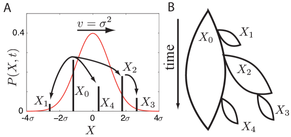
Figure 1: A novel mutation needs to recombine onto fitter genetic backgrounds to become established and eventually fix. Panel A: The distribution in fitness of the population moves towards higher fitness with velocity $v=\sigma^{2}$. The new mutation, illustrated by the black bars, has to switch backgrounds by recombination to keep up with the moving wave of the population fitness distribution. Panel B: Initially, the novel mutation is present on a single genetic background with fitness $X_{0}$, struggling not to go extinct. Recombination can transfer the mutated allele onto a new background, e.g. from $X_{0}$ to $X_{1}$, and spawn a daughter clone which starts an independent struggle against extinction. The mutation establishes if at least one branch survives indefinitely. The figure shows the complementary case of an unsuccessful mutation: all branches die out. The probability of establishment, $w(X,t)$, depends on the fitness $X$ of the genome in which the mutation arose and is a solution to Eq. (2).

The establishment probability at a time $t-dt$ of descendants of a genome of fitness $X$, defined as $w(X,t-dt)$, is simply related to that at time $t$ Barton (1995b):

$$\begin{split}w(X,t-dt)=&w(X,t)-dt[D+B(X,t)+r]w(X,t)+dtB(X,t)(2w(X,t)-w(X,t)^{2})\\ &+dt\ r\int dYK(X,Y,t)w(Y,t)\end{split}$$ (1)

where $D=1$ is the death rate and $B(X)=1+X-\bar{X}(t)$ the birth rate. After a division, either of the two offspring has a probability $1-w$ of extinction: hence $2w-w^{2}$ of at least one of these offspring fixing. For a low-frequency allele conferring additional fitness $s$ on a genomic background with fitness $X$, we have $B=1+X-\bar{X}(t)+s$.

In a sufficiently large population the adaptation process will proceed in a steady manner leading to a fitness distribution of constant width translating towards higher fitness as a “traveling wave” (Tsimring et al., 1996) with the velocity set by the rate of increase of the mean fitness $v=\frac{d}{dt}{\bar{X}}(t)$. We make the Ansatz that the distribution of fitnesses of the population around its mean $\bar{X}(t)$ does not fluctuate substantially and that the distribution is close to gaussian. These are analogous to “mean-field” approximations which must be justified a posteriori. We expect that such approximations will become valid for sufficiently large populations, but how this occurs and how large the population must be, is not clear a priori: we discuss this below.

In the traveling wave population, the establishment probability depends on time only via ${\bar{X}}(t)$. Hence we measure fitness relative to ${\bar{X}}(t)=vt$, defining $x\equiv X-{\bar{X}}(t)$, and seek an otherwise time-independent solution of the form $w(x)=w(X-vt)=w(x,t)$. (The properties of $w(X,t)$ and $K(X,Y,t)$ do not change by this shift of variables other than becoming time independent relative to a moving reference $\bar{X}(t)$. We therefore use the same symbols for $w(x)$ and $K(x,y)$ in the moving frame.) Using $\partial_{t}w(X-vt)=-v\partial_{x}w(x)$, the establishment probability, $w(x)$, then obeys

$$\begin{split}v\partial_{x}w(x)=r\int dyK(x,y)w(y)+(x+s-r)w(x)-(1+x+s)w(x)^{2}\ .\end{split}$$ (2)

In many cases of interest, selection is only important on timescales much longer than the generation time. In that case $x+s$ in the prefactor of the quadratic term is negligible compared to the inverse generation time, which is $1$ in our units. Eq. (2) then simplifies to

$$\begin{split}(v\partial_{x}-x+r)w(x)-r\int dyK(x,y)w(y)\ =\ sw(x)-w(x)^{2},\end{split}$$ (3)

We have written this in a suggestive form. The left hand side of Eq. (3) defines the linear operator ${\cal J}$ acting on $w(y)$. At very high recombination rates, we will obtain that $w(x)\sim(1+2x/r)$ which is almost independent of $x$ for $x\ll r$. In this limit, the ${\cal J}$ acting on $w(y)$ vanishes and the population average establishment probability is just the solution to the right-hand side, giving simply $w(x)\approx s$. This is the conventional result (obtained by the simple branching process) in the absence of linkage to the rest of the genome. More generally, the fixation probability of a new mutation which can arise in any individual is the population average of the $x$-dependent establishment probability over the approximately gaussian distribution of the fitness, $x$:

$$P_{e}\approx\int\frac{dx}{\sqrt{2\pi\sigma^{2}}}e^{-\frac{x^{2}}{2\sigma^{2}}}w(x)$$ (4)

Equation (3) has an important property. Its left hand side is zero upon averaging with respect to the population distribution $P(x)=\frac{1}{\sqrt{2\pi\sigma^{2}}}e^{-x^{2}/2\sigma^{2}}$ (as is readily confirmed by direct integration using $v=\sigma^{2}$ and $\int dxK(x,y)P(x)=P(y)$, see above). This property originates from the fact that in the deterministic limit (without the additional mutation, $s$), the population dynamics has $P(X,t)=P(X-vt)=P(x)$ as a traveling wave solution (Rouzine and Coffin, 2005) — the initial rationale for assuming a gaussian form. As a consequence, averaging Eq. (3) yields a “solvability condition”

$$\int\frac{dx}{\sqrt{2\pi\sigma^{2}}}e^{-\frac{x^{2}}{2\sigma^{2}}}\left(sw(x)-w(x)^{2}\right)=0$$ (5)

which, when combined with Eq. (4), provides another expression for the establishment probability:

$$sP_{e}=\int\frac{dx}{\sqrt{2\pi\sigma^{2}}}e^{-x^{2}/2\sigma^{2}}w(x)^{2}\ .$$ (6)

This equation together with Eq. (3) describes the “surfing” of a beneficial allele (and far more often its drowning!) — the processes illustrated by figure 1 — under the assumption that the distribution of fitness in the population is sufficiently close to gaussian. The latter holds when the large number of alleles at different loci are only weakly correlated: we justify this Ansatz below.

I.2 Models of recombination

The recombination kernel $K(x,y)$ depends on the recombination model. For the free recombination model, the fitness of the offspring resulting from a mating of two parents with fitness $x$ and $z$ is again Gaussian distributed with mean $(x+z)/2$ and variance $\sigma^{2}/2$. Averaging over the fitness $z$ of the mate, which is Gaussian distributed with variance $\sigma^{2}$, results in the recombination kernel

$$K(x,y)=\sqrt{{2\over 3\pi\sigma^{2}}}e^{-\ {2(y-{x\over 2})^{2}\over 3\sigma^{2}}}\ .$$ (7)

In the communal recombination model, the fitness of the recombinant is a random sample from the population (assuming gaussianity and linkage equilibrium). In that case, we have

$$K(x,y)=\frac{1}{\sqrt{2\pi\sigma^{2}}}e^{-\frac{y^{2}}{2\sigma^{2}}},$$ (8)

i.e. the recombination kernel becomes independent of $x$ and equation Eq. (3) becomes mathematically much simpler.

Within the minimal recombination model, the probability per unit time of any particular locus being transferred is $r$ and the sections are assumed small enough that they contain at most one segregating locus. From the point of view of a single mutant, there are two processes: either it can be transfered to another genome, which is effectively like the recombination process in the communal recombination model, or other sections can be transfered into its genome gradually changing its fitness. With small sections transfered the fitness of the genome undergoes a random walk with bias towards the average fitness. The corresponding recombination operator is then

$$r\int dyK(x,y)w(y)=r\int\frac{dy}{\sqrt{2\pi\sigma^{2}}}e^{-\frac{y^{2}}{2\sigma^{2}}}w(y)+r[\sigma^{2}\frac{d^{2}w}{dx^{2}}-x\frac{dw}{dx}]\ .$$ (9)

This form of the recombination operator is derived in the Appendix C. Note that for the minimal recombination model the recombination operator acting on $P(x)$ is different from the adjoint operator acting on $w(y)$.

II Results

II.1 Fixation probability and rate of adaption

To calculate the rate of adaptation, we solved Eq. (3) and obtained expressions for the average fixation probability $P_{e}$ of a beneficial mutation, which is of the form $P_{e}=\sigma p_{e}(\tilde{r},\tilde{s})$, where $\tilde{s}=s/\sigma$ and $\tilde{r}=r/\sigma$ are the selective advantage of the beneficial mutation and the outcrossing rate rescaled by the to-be-determined width of the fitness distribution $\sigma$. The expression for $P_{e}$ is used later to calculate $\sigma^{2}$ in a self-consistent manner. The derivation of the expressions for $P_{e}$ in the different models are given in the following section. In the limit $s\ll r$, our primary focus, we find for the free recombination model

$$p_{e}(r/\sigma,s/\sigma)=\begin{cases}\vspace{0.2cm}\frac{\sigma^{2}\log(cr/s)}{sr\sqrt{2\pi}}e^{-\frac{\sigma^{2}}{2r^{2}}\log^{2}(cr/s)}&s\ll r\ll\sigma\\ \frac{s}{\sigma}\left(1-4\frac{\sigma^{2}}{r^{2}}+\ldots\right)&r\gg\sigma\end{cases}$$ (10)

with $c$ a coefficient. At small $r$, the fixation probability decreases very rapidly with decreasing $r$. This stems from the fact that mutations in individuals from the high fitness tail of the Gaussian fitness distribution have an exponentially greater chance of fixing than those in the bulk. At large $r$, by contrast, the genetic background on which the mutation arises plays only a minor role, since the rate of switching background is larger than the selection differentials. While starting out on a fit background gives a mutation a slight advantage, mutations on any background have a significant chance of fixing. For large $r$, the result for $P_{e}$ is therefore given by small perturbations of the result without background interference: $P_{e}\approx s$.

The expressions for $P_{e}$ presented above depend on the variance in fitness $\sigma^{2}$. In an evolving population the variance is not a free parameter. When the effects of mutation on the bulk of the fitness distribution can be neglected, as they can here, the variance is equal to the rate of adaptation, $v$. The rate of adaptation, in turn, is given by product of the rate at which beneficial mutations enter the population $NU_{b}$, the magnitude of their effect $s$ and their probability of fixation.

$$v=NU_{b}s\sigma p_{e}(r/\sigma,s/\sigma)=\sigma^{2}$$ (11)

The rate of adaptation, $v$, can therefore be obtained by solving self-consistently for $\sigma$ in the above equations. Substituting our result for $P_{e}$ and ignoring logarithmic factors in the arguments of large logarithms, we find, for the free recombination model,

$$v\approx\begin{cases}\vspace{0.2cm}2s^{2}\left(\frac{r}{s}\right)^{2}\frac{\log NU_{b}}{\log^{2}r/s}&1\ll\frac{r^{2}}{s^{2}}\ll NU_{b}/\log{NU_{b}}\\ NU_{b}s^{2}\left(1-\frac{4NU_{b}s^{2}}{r^{2}}+\ldots\right)&\frac{r^{2}}{s^{2}}\gg 4NU_{b}\end{cases}$$ (12)

Contrary to intuition, $v$ is proportional to $\log NU_{b}$ rather than $NU_{b}$ both for low $r$ at fixed $NU_{b}\gg 1$, and at fixed $r$ for sufficiently large populations sizes, $N$. This indicates that the interplay between mutations — especially their collective effects on fluctuations — is limiting the rate of adaptation Gillespie (2001). As in the asexual case, because of interference between mutations, only a small fraction $\sim\log(NU_{b})/NU_{b}$ of the beneficial mutations fix — the rest are wasted. However, this fraction increases with increasing rate of recombination leading to $v$ increasing as $\sim r^{2}\log NU_{b}$, until it saturates at $NU_{b}s^{2}$, which is the limit of independently fixating mutations. In this high recombination limit, the rate of adaptation is limited simply by the supply of beneficial mutations $NU_{b}$. Very similar results for the dependence of $v$ on $r$ and $N$ are obtained for the communal recombination model, differing only by coefficients inside logarithms and by correction terms.

In the minimal recombination model, for which only one locus is exchanged at a time, the behavior is slightly different. For the fixation probability, we find

$$P_{e}\sim e^{-\sigma^{2}/2r^{2}+s\sigma^{2}/r^{3}}\ .$$ (13)

In contrast to the other models for which recombination results in a macroscopic change of the genotype, the minimal recombination model only changes one locus at a time. This results in a slightly weaker dependence of $P_{e}$ on the recombination rate for $r\gg s$. Self-consisting the fitness variance as before determines the speed of adaptation to be

$$v\approx 2r^{2}\log(NU_{b})(1+2s/r)\ .$$ (14)

Surprisingly, this result in essentially independent of $s$ for $r\gg s$: the larger increase in the fitness per sweep is almost perfectly canceled by the decrease in establishment probability. Note that this model is defined with recombination rate $r$ per locus so that the total number of recombinations in time $1/r$ is far more than in the other models. But the time for turnover of the genome and loss of linkage is of order $1/r$ and thus $r$ is the useful quantity to compare with the other models.

II.2 Simulations

In writing down Eq. (3) for the establishment probability of a beneficial mutation, we have assumed that the distribution of fitness in the population is gaussian and that correlations and fluctuations are negligible. Thus it is useful to compare the analytic results to individual-based simulations of an evolving population. In our simulations, we use a discrete generation scheme, where each individual produces a Poisson distributed number of gametes with parameter $\exp(X-\bar{X}+\alpha)$. The population size, $\tilde{N}$, is kept approximately constant with an average of $N$ by adjusting the overall rate of replication through $\alpha=(1-\tilde{N}/N)\log 2$. Each individual is represented by a string of integers, where each bit represents one locus. Recombination, approximating the free recombination model, is implemented as follows: Each generation, gametes are randomly placed into a pool of asexual gametes with probability $1-r$ and into a pool of sexual gametes with probability $r$. The asexual gametes are placed unchanged into the next generation. The sexual gametes are paired at random and their genes reassorted to produce haploid offspring. Whenever one locus becomes monomorphic — via fixation or extinction of an allele — , one individual is chosen at random and a mutation introduced at that specific locus. This allows us to make optimal use of the computational resources by keeping as many polymorphic loci as possible. However, this scheme renders the beneficial mutation rate, $U_{b}$, a dependent quantity which, as shown in Fig. 2, increases with $L$ and decreases with $r$. The effective total rate for new beneficial mutations, $NU_{b}$, can be determined simply by measuring the average rate at which the new mutations are introduced (which, the way the simulations are done, is the sum of the extinction and fixation rates).

Figure 2 shows the mean establishment probability as a function of the outcrossing rate $r$, for different values of $L$ which is roughly proportional to $NU_{b}$ (see above). The establishment probability is small at small $r$ but increases sharply and saturates at high $r$ at $P_{e}=2s$ — the usual single-locus result. The upturn of $P_{e}$ occurs at larger $r$ for larger $NU_{b}$, in accord with the prediction that the high recombination limit is reached when $r$ substantially exceeds $\sigma$. The agreement between the analytic predictions in the gaussian Ansatz (via numerical solution of Equation 3) and the simulation improves as $NU_{b}$ increases, suggesting that, as we expect, the approximations used become valid for large populations. Note, however, that the corrections to the asymptotic results are quite large as the basic small parameter of the gaussian Ansatz is inversely proportional to $\log(NU_{b})$. The right panel of Figure 2 shows $w(x)$, i.e. the establishment probability of a mutation arising on background $x$, measured in simulations together with the predictions obtained from numerical solution of Eq. (3). At outcrossing rates much larger than $\sigma$, the fixation probability increases only slightly with the background fitness and all new mutations have a substantial chance — of order $s$ — to establish. With decreasing $r/\sigma$, the establishment probability becomes a steeper function of the background fitness and only those mutations arising on high fitness backgrounds have a significant chance of establishment. Note that at $r/\sigma\approx 1$, $w(x)$ measured in simulations decays less rapidly at small $x$ than the solution of Eq. (3). These deviations are probably due to fluctuations of the high fitness edge and the width of the distribution which are ignored in the analysis. However, as discussed below, such fluctuations decrease with increasing $NU_{b}$ as long as $r\gg s$.

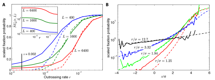
Figure 2: Fixation probabilities in recombining populations. Panel A shows the mean fixation probability normalized to the value in the high recombination limit as a function of $r$ for three different genome sizes $L$ (with $s=0.002$, $N=20000$). The effective rate of beneficial mutations $NU_{b}$ is shown in the inset (see main text). The scaled fixation probability in the simulation (solid lines) is calculated as $v/2NU_{b}s^{2}$ and compared to the analytic results for the scaled establishment probability $P_{e}(r,\sigma)/s$ (dashed lines). The latter are obtained through numerical solution of Eq. (3) using $\sigma^{2}$ observed in simulations. The agreement between simulations and the analytic approximation improves with increasing $L$, i.e. increasing $NU_{b}$, as expected. Panel B: The scaled fixation probability as a function of the rescaled background fitness $x/\sigma$ (relative to the mean). The solid lines are simulation results for $w(x)$ divided by $2s$ using $L=6400$ and $r=0.512,\ 0.128,\ 0.064$ and 0.032: the corresponding values of the key ratio $r/\sigma$, which determines the shape of $w(x)$, are indicated in the figure. The dashed lines are predictions for $w(x)/s$ obtained via numerical solutions of Eq. (3). Note that the simulation data becomes noisy when the frequency of $x$ in the population is around $1/N$.

III Analysis of Establishment Probability

We now turn to a derivation of the results given for the establishment probability in Eqs. (10) and (13), which requires solving Eq. (3). We first study the case of $s\ll r\ll\sigma$ applicable, as we shall see, for very large populations. We proceed by analysing Eq. (3) in different regimes of $x$. At large positive $x-r\gg\sigma$, the equation reduces to $(x-r)w(x)\approx w^{2}(x)$ with solution $w_{>}(x)\approx x-r$, as illustrated in figure 3. In this regime, $w(x)$ is independent of the recombination model and is simply given by the establishment probability of a mutation in the absence of any gains from recombination (but with the clonal growth rate reduced by $r$ due to recombination). Establishment is driven by clonal expansion and contributions from recombination are negligible. (But we shall see that there are almost no individuals in the population with such high fitness.) In the opposite regime, at large negative $x$, $w(x)$ is small and the quadratic term, as well as the perturbation $sw(x)$ can be neglected. The resulting linear equation for $w_{<}(x)$ valid for small $x$ is

$$(v\partial_{x}-x+r)w_{<}(x)-r\int dyK(x,y)w_{<}(y)\ =0\ .$$ (15)

In this regime, the solution depends sensitively on the recombination model. This is intuitive, since the only — and very unlikely — way for a mutation at $x\ll 0$ to fix is to recombine onto better backgrounds. We will verify below for each model separately, that the crossover from the linear regime, $w_{<}(x)$, to the saturated behavior at large $x$, $w_{>}(x)$, occurs rather sharply around $x/\sigma=\Theta\gg 1$. At intermediate $\sigma<x<\sigma\Theta$, the establishment probability $w_{<}(x)$ increases steeply (while remaining small enough for the quadratic term to remain negligible). Individuals in this intermediate regime are much fitter than the average individual so that recombination usually leads to less fit offspring. Hence the recombination term is of secondary importance in this range and $w_{<}(x)$ is governed by the first term in Eq. (15). The solution to Eq. (15) is therefore of the form $w_{<}(x)=\phi(x)e^{(x-r)^{2}/2\sigma^{2}}$, where $\phi(x)$ is a slowly varying function that depends on the recombination model. This behavior can be interpreted in terms of the dynamics of a genotype with initial fitness $x$. The genotype will expand clonally with rate $x-r$, giving rise to approximately $n_{x}\sim e^{(x-r)t-vt^{2}/2}$ unrecombined descendants after $t$ generations. Since each of these could give rise to a lineage which will fix, in this regime $w(x)$ is proportional to $\int n_{x}(t)dt$, which increases rapidly with $x$. This is valid up to just below the crossover where the quadratic term, $w(x)^{2}$, starts to be important, see fig. 3.

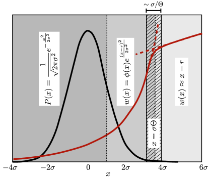
Figure 3: Asymptotics of the establishment probability. The fitness distribution $P(x)$ of the population is shown in black, a sketch of the establishment probability, $w(x)$, is shown in red for $r\ll\sigma$. At low $x$, $w(x)$ is small and depends sensitively on the recombination model, at intermediate $\sigma<x<\sigma\Theta$, $w(x)$ increases sharply as $\sim e^{\frac{(x-r)}{2\sigma^{2}}}$, modulated by a slowly varying function $\phi(x)$ which depends on the recombination model. At still larger $x$, beyond $\sigma\Theta$, the quadratic term in Eq. (3) becomes important, forcing $w(x)$ to saturate at $x-r$. The width of the crossover region is of the order of $\sigma/\Theta$.

Note that the amplitude of $w_{<}(x)$ is left undetermined by the homogeneous linear equation (15) and hence the location $\Theta$ of the crossover is not fixed. To insure that $w(x)$ solves the complete Eq. (3), we need to impose the “solvability condition” Eq. (5) as an additional constraint. The solvability condition involves the first and second moment of $w(x)$ with respect to the fitness distribution $P(x)$. The first moment is dominated by small and intermediate $x$ since $P(x)w(x)$ decreases with $x$. The second moment, however, is dominated by a narrow range of width $\sim\sigma/\Theta\ll\sigma$ around the crossover point $\sigma\Theta$: for $x\approx\sigma\Theta$, $P(x)w_{<}(x)^{2}$ increases rapidly with $x$, while $P(x)w_{>}(x)^{2}$ decreases rapidly. The “solvability condition” (5) then becomes

$$sP_{e}\approx\frac{\sigma\Theta}{\sqrt{2\pi}}e^{-\Theta^{2}/2}$$ (16)

giving us a relation between $P_{e}$ and $\Theta$. To analyze the behavior of the various models it is convenient to rescale the rates and fixation probabilities as

$$\chi=x/\sigma,\ \ \ \tilde{r}=r/\sigma,\ \ \ \tilde{s}=s/\sigma,\ \ {\rm and}\ \ \tilde{w}(\chi)=w(\chi\sigma)/\sigma\ .$$ (17)

Utilizing the transform,

$$\Omega(z)\equiv\int_{-\infty}^{\infty}\frac{d\chi}{\sqrt{2\pi}}e^{-\frac{(\chi-z)^{2}}{2}}\tilde{w}(\chi)\ ,$$ (18)

turns out to be informative: note that the scaled fixation probability is $p_{e}\equiv P_{e}/\sigma=\Omega(z=0)$. By integrating the rescaled Eq. (3) over the kernel $\frac{1}{\sqrt{2\pi}}e^{-\frac{(\chi-z)^{2}}{2}}$, we obtain an equation for $\Omega(z)$ of the form

$${\cal L}\Omega=\int_{-\infty}^{\infty}\frac{d\chi}{\sqrt{2\pi}}e^{-\frac{(\chi-z)^{2}}{2}}\ {\cal J}\ \tilde{w}(\chi)=\tilde{s}\Omega(z)-\int_{-\infty}^{\infty}\frac{d\chi}{\sqrt{2\pi}}e^{-\frac{(\chi-z)^{2}}{2}}\tilde{w}(\chi)^{2}\,$$ (19)

which defines for each model a linear operator $\cal L$ acting on $\Omega(z)$ (${\cal J}$ is the linear operator defined by the left hand side of Eq. 3)). The integral over $\tilde{w}(\chi)^{2}$ is again dominated by the crossover region and can be evaluated using $\tilde{w}(\Theta)\approx\Theta$ and the (scaled) crossover width $\sim\Theta^{-1}$

$${\cal L}\Omega\approx\tilde{s}\Omega(z)-\frac{\Theta}{\sqrt{2\pi}}e^{-(\Theta-z)^{2}/2}=\tilde{s}\Omega(z)-\tilde{s}\Omega(0)e^{\Theta z-z^{2}/2}.$$ (20)

The last step was obtained by substituting Eq. (16). The condition that the solution $\tilde{w}_{<}(\chi)$ joins smoothly to the saturated solution $\tilde{w}_{>}(\chi)$ and hence only grows slowly for large $\chi$, translates into the condition that $\Omega(z)$ does not diverge at any fixed $z$: it should be an analytic function of $z$. We now examine separately the different models, simplest first.

III.1 Communal recombination model.

In the communal recombination model, the genotypes of offspring are independent of their parental fitness, which makes this model particularly simple. It can, in fact, be solved exactly, as shown in Appendix A, or, in the regimes of interest, by matched asymptotic expansions. But it is more instructive to proceed with the approximate but more general and asymptotically exact analysis outlined above. The equation for $\Omega(z)$ reads

$${\cal L_{C}}\Omega\equiv(\tilde{r}-z)\Omega(z)-\tilde{r}p_{e}=\tilde{s}\Omega(z)-\tilde{s}\Omega(0)e^{z\Theta-z^{2}/2}\,$$ (21)

which can be solved trivially. But in general it has a pole at $z=\tilde{r}-\tilde{s}$. This pole has to be canceled, since we know that $\tilde{w}(\chi)$ saturates at $\chi=\Theta$ and $\Omega(z)$ cannot develop a singularity. Hence, we must have $e^{\Theta(\tilde{r}-\tilde{s})-(\tilde{r}-\tilde{s})^{2}/2}=\tilde{r}/\tilde{s}$ to eliminate the pole. Solving for $\Theta$ and substituting it into the solvability condition (16) yields

$$p_{e}\approx\ \frac{\log(\tilde{r}/\tilde{s})}{\tilde{s}(\tilde{r}-\tilde{s})\sqrt{2\pi}}e^{-\frac{1}{2(\tilde{r}-\tilde{s})^{2}}\left(\log(\tilde{r}/\tilde{s})+\frac{(\tilde{r}-\tilde{s})^{2}}{2}\right)^{2}}\approx\frac{\log(\tilde{r}/\tilde{s})}{\tilde{s}^{1/2}\tilde{r}^{3/2}\sqrt{2\pi}}e^{-{\log^{2}(\tilde{r}/\tilde{s})\over 2\tilde{r}^{2}}}\ .$$ (22)

The last approximate equality is correct to leading order in $\tilde{s}/\tilde{r}\ll 1$.

III.2 Free recombination model

In the free recombination model, the offspring obtains on average half of its genome from either parent. The parent carrying the new allele mates with a random member of the population: thus after recombination the average fitness of the genotype carrying the new allele is half as far from the population mean fitness as it was before recombination. As a result of this correlation between parents and offspring, the operator ${\cal L_{I}}$ for the free recombination model is more complicated and couples $\Omega(z)$ to $\Omega(z/2)$.

$${\cal L_{I}}\Omega\equiv(\tilde{r}-z)\Omega(z)-\tilde{r}\Omega(z/2)\approx\tilde{s}\Omega(z)-\tilde{s}\Omega(0)e^{z\Theta-z^{2}/2}$$ (23)

where, as before, $p_{e}=\Omega(0)$. Neglecting the $e^{-z^{2}/2}\approx 1$ on the right hand side (we need only consider $z\ll 1$ since $\tilde{r}\ll 1$), we can analyze this as a power series in $z$ writing $\Omega(z)=\sum_{n}\Omega_{n}z^{n}$ finding

$$\frac{\Omega_{n}}{\Omega_{0}}=\prod_{k=1}^{n}\frac{1}{\tilde{r}-\tilde{s}-\tilde{r}2^{-k}}-\tilde{s}\sum_{j=1}^{n}\frac{\Theta^{j}}{j!}\prod_{k=j}^{n}\frac{1}{\tilde{r}-\tilde{s}-\tilde{r}2^{-k}}\ .$$ (24)

As the first part would yield ratios of successive terms which approach $1/(\tilde{r}-\tilde{s})$ for large $n$ and again induce a pole at $z=\tilde{r}-\tilde{s}$, this has to be canceled by the second inhomogeneous term. The condition for convergence (up to well beyond the “almost-pole” at $\tilde{r}-\tilde{s}$) is that $\Omega_{n}(\tilde{r}-\tilde{s})^{n}\to 0$ for $n\to\infty$ which requires that

$$1=\tilde{s}\sum_{j=1}^{\infty}\frac{\Theta^{j}}{j!}\prod_{k=1}^{j-1}(\tilde{r}-\tilde{s}-\tilde{r}2^{-k})\approx e^{\Theta(\tilde{r}-\tilde{s})}\frac{\tilde{s}}{\tilde{r}}\prod_{k=1}^{\infty}(1-2^{-k}).$$ (25)

The last approximate equality is accurate when $\tilde{s}\ll\tilde{r}$ and hence $\Theta(\tilde{r}-\tilde{s})\gg 1$. Thus we must have

$$\Theta\approx\frac{\log(c\tilde{r}/\tilde{s})}{\tilde{r}-\tilde{s}}$$ (26)

with the order-unity coefficient $c=1/\prod_{k=1}^{\infty}(1-2^{-k})$. We thus obtain $p_{e}$ very similar to the communal recombination model,

$$p_{e}\approx\frac{\log(c\tilde{r}/\tilde{s})}{\tilde{s}(\tilde{r}-\tilde{s})\sqrt{2\pi}}e^{-\log^{2}(c\tilde{r}/\tilde{s})/2(\tilde{r}-\tilde{s})^{2}}\ .$$ (27)

Note that $\Omega(z)$ is approximately the Laplace transform of $\phi(\chi)=\tilde{w}(\chi)e^{-\chi^{2}/2}$, which can be analyzed perturbatively for small $\tilde{r}$, see Appendix B. This expansion in $\tilde{r}$ reveals the most probable — least unlikely — path of a mutation on a typical initial background to successively better backgrounds and establishment.

III.3 Minimal recombination model

The minimal recombination model can be analyzed similarly: ${\cal L}_{T}$ is now a differential operator, and we have

$${\cal L_{T}}\Omega\equiv(\tilde{r}-z)\Omega-\tilde{r}p_{e}+\tilde{r}z\frac{d\Omega}{dz}\approx\tilde{s}\Omega-\tilde{s}\Omega(0)e^{z\Theta}\ .$$ (28)

This can be explicitly integrated and the behavior for $1\gg z>{\cal O}(\tilde{r})$ found to involve linear combinations of $e^{z/\tilde{r}}$ and $e^{z\Theta}$. For $\tilde{s}\ll\tilde{r}$, the condition that the solution matches correctly onto the non-linearly saturated form for $\chi\approx\Theta$, can be shown to be that these two exponentials are almost the same. This yields the condition $\Theta\approx 1/\tilde{r}$. In contrast to the other models, $\tilde{s}$ only gives corrections to $\Theta$. The fixation probability is then found to be

$$P_{e}\sim e^{-1/2\tilde{r}^{2}+\tilde{s}/\tilde{r}^{3}}$$ (29)

which yields a different form for the speed of evolution:

$$v\approx 2\tilde{r}^{2}\log(N\mu)(1+2\tilde{s}/\tilde{r})\ .$$ (30)

III.4 High recombination rates

In the limit of high recombination rate, the crossover to the saturated solution $\tilde{w}_{<}(\chi)$ occurs far out in the “nose” (high fitness tail) of the population distribution — further out than any individuals are likely to be. In this regimes, the assumption that $\int d\chi e^{-\chi^{2}/2}\tilde{w}(\chi)^{2}$ is dominated by the crossover region is no longer justified.

To analyse this high $r$ regime, we can make use of the expansion of $\Omega(z)=\sum_{n}z^{n}\Omega_{n}$, which is equivalent to expanding $\tilde{w}(\chi)$ in Hermite polynomials $\tilde{w}(\chi)=\sum_{n}\Omega_{n}H_{n}(\chi)$, where the $H_{n}(\chi)=(-1)^{n}e^{\chi^{2}/2}\partial_{\chi}^{n}e^{-\chi^{2}/2}$. In the limit of $\tilde{r}\gg\tilde{s}$, the second term in Eq. (24) can be neglected for the first few coefficients and we have $\Omega_{n}/\Omega_{0}=\prod_{l=1}^{n}\frac{1}{\tilde{r}(1-2^{-l})}$ (for the communal recombination model we have $\Omega_{n}/\Omega_{0}=\tilde{r}^{-n}$). The value of $\Omega_{0}=p_{e}$ has to be determined by the solvability condition $\tilde{s}p_{e}=\int d\chi/\sqrt{2\pi}e^{-x^{2}/2}\tilde{w}(\chi)^{2}$. From the orthogonality of the Hermite polynomials one finds that the right hand side is simply $\sum_{n}n!\Omega_{n}^{2}$. Hence, we find for the fixation probability the formal expression

$$p_{e}=\Omega_{0}=\tilde{s}\left(1+\sum_{n=1}n!\prod_{l=1}^{n}\frac{1}{\tilde{r}^{2}(1-2^{-l})^{2}}\right)^{-1}$$ (31)

The $n!$ would cause the sum to diverge if it extended to infinity. But for large $\tilde{r}$, this is a valid asymptotic series, which can be truncated at any finite number of terms. To zeroth order, one finds in both models $P_{e}=\sigma\tilde{s}=s$ which is simply the result in a homogeneous population. Including the first two non-trivial correction terms, one finds

$$P_{e}= s\left(1-4\tilde{r}^{-2}+\frac{16}{9}\tilde{r}^{-4}+\cdots\right)\quad \mathrm{free~{}recombination~{}model}$$ (32)

$$P_{e}= s\left(1-\tilde{r}^{-2}-\tilde{r}^{-4}+\cdots\right)\quad \mathrm{communal~{}recombination~{}model}$$

[Note that the divergence of the expansion for large $n$, for which this approach breaks down, is related to the singular dependence of $p_{e}$ on $1/\tilde{r}$ for small $\tilde{r}$ discussed above.] For the minimal recombination model, the behavior for large $r$ is similar and the expansion in inverse powers of $\tilde{r}$ can be analyzed: we do not carry this out here.

III.5 Range of validity of analysis

Throughout the analysis, we have assumed that the fitness distribution of individuals in the population, $P(x=X-\bar{X}(t))$, is gaussian, and also that of recombinant offspring. Crucially, for the analysis, we assumed that it remains gaussian in the high-fitness nose of the distribution all the way to the crossover point $\Theta$ which controls the establishment probabilities. We need to justify this Ansatz. First, as noted earlier, we observe that a gaussian fitness distribution is the exact traveling-wave solution to the linear recombination model in the absence of fluctuations: the gaussian approximation should thus be valid throughout the bulk of the distribution in the limit of very large populations. Second, in the absence of fluctuations (or epistatic interactions which we are ignoring in any case) the frequencies of alleles at different loci are independent. And third, if the establishment probabilities of different beneficial mutations are independent, then it can be shown that the resulting Poisson process of the establishments together with random combining of the alleles with their corresponding frequencies leads to a distribution of fitnesses whose logarithm averaged over the establishment times, $\langle\log(P(x))\rangle$, is exactly parabolic — corresponding to a gaussian distribution. However, due to fluctuations and correlations, the distribution of fitnesses will be neither exactly gaussian nor exactly time-independent and we must check that the non-fluctuating gaussian is a good enough approximation far enough out in the nose in the large $N$ regimes of interest.

We first check that the sampling of the distribution due to the finite population size is sufficient. A population of size $N$ samples a close-to-gaussian distribution only out to about $\sigma\sqrt{2\log N}$ ahead of the mean. But this implies that, with the fitnesses of individuals only weakly correlated, the crossover region near $\Theta$ is indeed well sampled by the population since

$$\Theta\approx\sigma\frac{\log cr/s}{r}=\sqrt{2\log NU_{b}}<\sqrt{2\log N}\ .$$ (33)

The last inequality is valid when the rate of beneficial mutations per genome per generation, $U_{b}$, is small as is surely always the case: there are then of order $1/U_{b}$ individuals in the population with fitnesses in the crucial crossover region of the establishment probabilities. Furthermore, the Gaussian shape of the fitness distribution will be a good approximation when the number of polymorphic loci that contribute substantially to the fitness variance is large. However, the total number of established polymorphic loci is dominated by low frequency alleles. (The total number of polymorphic loci is much higher still, but almost all of these are not established and destined to soon go extinct.) Nevertheless, there are sufficiently many polymorphic sites with high enough frequencies that they contribute substantially to the fitness distribution. Since sweeps occur at rate $v/s$ and since a sweeping allele is at intermediate frequencies for a few times $1/s$ generations, the number of loci, $K$, contributing substantially to the variance is of order $v/s^{2}\sim(r/s)^{2}\log(NU_{b})$. For $r\gg s$ these $K$ loci are approximately in linkage equilibrium, giving rise to a gaussian fitness distribution with corrections to parabolic $\log(P(x))$ of order $(x/\sigma)^{2}/K$. At the crossover point, $\sigma\Theta$, it can then be checked that the corrections to $P(x)$ are small as long as $r\gg s\sqrt{\log NU_{b}}$. We thus expect that this is the condition for validity of the gaussian Ansatz from which our analytic predictions are obtained. A more detailed analysis of the effects of fluctuations, in particular in the crucial “nose” of the distribution, is left for future work.

IV Discussion

We have analyzed in several simple models the dependence of the speed of adaptation on the rate of recombination and the population size, focusing on the particularly interesting behavior in the wide range of outcrossing rates $s\sqrt{\log NU_{b}}\ll r<s\sqrt{NU_{b}/\log NU_{b}}$, or equivalently, on population sizes $NU_{b}\gg\frac{r^{2}}{s^{2}}\log(r/s)$. In the high recombination limit and moderate $N$ the conventional analysis of independent fixations holds and the rate of adaptation (and concomitantly the variance of fitness) are proportional to the total production rate of beneficial mutations, $NU_{b}$. In contrast, for large populations (with recombination rates in the intermediate regime) we find adaptation rate $v\sim r^{2}\log NU_{b}$. This change from linear to logarithmic dependence on $NU_{b}$ indicates that the rate of adaptation is limited by interference among multiple simultaneously segregating beneficial mutations rather than by the supply of beneficial mutations. This reduction in the rate of adaptation due to linkage is, qualitatively, the Hill-Robertson effect Hill and Robertson (1966). Most interestingly, while logarithmic in population size, the rate of adaptation increases with the rate of recombination as $r^{2}$. Hence our results confirm the heuristic arguments by Fisher and Muller and provide a quantitative framework for identifying conditions favoring sexual reproduction Barton and Charlesworth (1998); Rice (2002).

The rate of adaptation is determined by the dynamics of the linkage between new beneficial alleles and the spectrum of fitnesses of the rest of the genome. This results in most new mutations being eliminated by their linkage to modestly fit genomes which rapidly lose out with respect to the steadily increasing average fitness driven by the anomalously fit genomes. Only those alleles that either arise on very fit genomes or are lucky enough to recombine to make a very fit genome will survive long enough for their frequency to grow deterministically and sweep through the population. The logarithmic dependence on population size is similar to that found for purely asexual evolution when multiple beneficial mutations are present in the population (Desai and Fisher, 2007). But with $r>s$, recombination speeds up the adaptation by allowing new mutations that arise on modestly fit backgrounds to recombine to very fit backgrounds and thereby fix.

We have shown that the typical number of simultaneously segregating alleles at intermediate frequencies is on the order of $K\sim r^{2}/s^{2}\log NU_{b}$. For $r\gg s$, the number of possible combinations of these sweeping loci therefore dramatically exceeds the population size. This implies that the limit of “infinite” population size, for which each genotype is well-sampled is unattainable at fixed recombination and beneficial mutation rate. On the contrary, sampling becomes sparser and the benefits of recombination more pronounced in larger populations. The population size dependence of the beneficial effects of recombination has been a subject of considerable theoretical debate (Crow and Kimura, 1965; Maynard Smith, 1968; Barton and Otto, 2005). The increased advantage of sexual reproduction in large population has been demonstrated in model simulations by Iles et al. (2003). It has also been observed experimentally by Colegrave (2002), who studied this phenomenon in an evolution experiment with C. reinhardtii.

IV.1 Relationship to other recent work

The description of the spread of beneficial alleles in space as a traveling wave goes back to Fisher (1930). The notion that adaptation of a panmictic population can be described as a travelling wave in fitness was introduced by Kepler and Perelson (1995) and Tsimring et al. (1996). In these effectively deterministic models, the velocity of the pulse is determined by the size of the population through a modification of the deterministic solution at the high fitness edge — the “nose” or “front” — to approximate the crucial stochastic behavior near the nose Brunet and Derrida (1997). These concepts were applied to recombining populations by Rouzine and Coffin (2005) and Gheorghiu-Svirschevski et al. (2007) who studied the rate of (transient) adaptation when selection acts on standing variation. Cohen et al. (2005, 2006) studied continuing evolution with a large supply of beneficial mutations available in a model that is related to our “minimal recombination” model. Both approaches focused on the overall distribution of fitnesses within the population and the primary role of recombination they considered was to maintain a near gaussian shape of the fitness distribution, achieved by producing higher fitness individuals and thereby advancing the nose. Some of the results of the approximate analytic treatments are related to ours, including the $\log N$ scaling of the adaptation speed in certain regimes. Yet the actual underlying dynamics implicit in the approximations used are very different from what we find here and so is the dependence on parameters.

The key feature of the adaptation with substantial rates of recombination is the stochastic dynamics of new mutations. The probability that a new beneficial mutation will sweep to fixation is determined by its establishment probability: the probability that it escapes stochastic extinction. The establishment probability depends very strongly on the distribution of fitnesses of the genetic backgrounds with which the new mutation can be linked. As the distribution of fitness depends on the velocity, the steady-state velocity must be determined by matching the rate of establishment of new alleles with the velocity of the deterministic traveling wave describing the fitness distribution in the population. The latter is driven by the continuous incorporation of a large number of new sweeping alleles that have successfully established at earlier times. At any time there is thus a broad distribution of frequencies of the beneficial alleles. The primary problem with the earlier analysis is that the distribution and dynamics of individual allele frequencies is not treated directly and the approximations implicitly made for their forms are not consistent with the basic processes.

In contrast with the asexual traveling wave for which a description in terms of a simple traveling wave is valid (Desai and Fisher, 2007; Rouzine et al., 2008) and the diversity within the population can be ignored, with any amount of recombination, the diversity and distribution of allele frequencies is absolutely crucial. It matters a great deal whether the advance of the fitness wave occurs via small amounts of each of several new alleles, or all from a single allele. This information is lost by treatments in terms of the fitness distribution alone. Note that in general this is also true for adaptation from standing variation: beneficial alleles initially at low frequencies can be driven extinct by their linkage to different backgrounds. If all are initially at sufficiently high frequencies to avoid this fate, then neither linkage nor recombination play much role in the dynamics of the adaptation.

The models we have studied were inspired by facultatively mating organisms, in which outcrossing occurs at rate $r$. Barton and Coe (pers. comm.) have recently performed a related analysis for obligate sexual reproduction. In addition to a model with a linear genetic map (see below), they study the free and minimal recombination models, for which they find similar logarithmic dependence on the population size and mutation rate. Their discrete generation models with obligate mating do not reveal the dependence of the rate of adaptation on the outcrossing rate, one of the results of our analysis, but a similar behavior is implicit in their results.

IV.2 Extensions and open questions

In this paper we focused on the effect of recombination with $r>s$ in simple models of mating without chromosomal organization and without epistasis. We conclude by considering going beyond these simplifying limits.

We first consider decreasing the recombination rate. In comparing our analytic results on the free recombination model with the direct simulations we found good agreement at high recombination rates which confirms the accuracy of the simplifying assumptions made in analyzing the model (i.e.  Eq. (3)). At lower recombination rates we observed that our “mean-field” treatment of the recombination underestimates the rate of adaptation. This is due to the gradual appearance of “fat tails” in the distribution of fitness: specifically, the high fitness nose of the distribution decays more slowly than the gaussian assumed in the analysis. The fluctuations in the time of establishment of the currently intermediate frequency alleles becomes important. Some of the causes of this can be studied analytically. The primary effect is the smaller number of segregating loci — of order $v/s^{2}\sim r^{2}/s^{2}$ — at low recombination rates. As the ratio $r/s$ decreases further, the acquisition of further beneficial mutations near the nose of the distribution — which dominates the asexual evolution — starts to become important. Correlations between loci caused by this process and other sources, will also play important roles.

The behavior of the leading edge of the fitness distribution is known to be the key factor in determining the speed of adaptation in the asexual limit of $r\rightarrow 0$ (Desai and Fisher, 2007) and it will be of critical importance in the $r\ll s$ regime. A correct treatment of this regime, connecting with the known results for asexual adaptation (Desai and Fisher, 2007; Rouzine et al., 2008; Brunet et al., 2008), requires analyzing the diversity that is generated by the asexual process and the effects of small amounts of recombination on this. It is worth noting that within our approximations, for the low recombination regime with $r\ll s$, the branching process analysis yields an adaptation speed for all three models of the form $v\sim s^{2}\log(N\mu)/\log^{2}(s/r)$ which is a similar form to the asexual result, $v\approx 2s^{2}\log(N\sqrt{\mu s})/\log^{2}(s/\mu)$. This suggests that in spite of the breakdown of the assumptions, the approximations may give reasonable results, although not asymptotically accurate ones, even for $s\gg r\gg\mu$. But we leave this regime, which is particularly important for microbes with rare genetic exchange, for future investigations.

Our analysis has focused on the simple approximation of additive growth rate (equivalent to multiplicative fitnesses in a discrete-generation model). Some of the most interesting extensions of the present models would include epistasis — i.e. genetic interactions — which makes the effect of each allele explicitly dependent on its genetic background. This dependence can be very complex resulting in low heritability of fitness, in the sense that the fitness of recombinant progeny may be only weakly correlated with the fitness of the parents. Remarkably, in the limit of very strong epistasis (Neher and Shraiman, 2009) the establishment probability of an allele is described by a model which reduces to the communal recombination model described above. The speed of adaptation is, however, determined by a different self-consistency condition which will be presented elsewhere. In general, how to setup — never mind analyze! — instructive models of evolutionary dynamics with epistasis between many segregating loci, is largely an open field.

Another important simplification in the free recombination model studied here is the random reassortment of the parental alleles ignoring the physical arrangement of the genes. More realistic models would account for the linear arrangement of genes on the chromosomes such that chromosomal proximity implies low recombination rate. In this case, the number of independently transmitted loci in the event of mating is the product of the number of chromosomes and the crossovers per chromosome. When the number of substantially polymorphic loci is sufficiently large, the free recombination approximation will certainly break down. But in facultatively mating organisms where periods of asexual reproduction are interspersed by outcrossing events much reassortment can occur. Indeed, some facultative outcrossers have high crossover rates (e.g. S.cerevisiae Mancera et al. (2008)). In this case the free recombination model can have a reasonable regime of validity. More generally, the fact that our three rather different models yield similar behavior for the adaptation rates at large population sizes suggests that the forms of the dependence on parameters — especially speed proportional to $\log(NU_{b})$ — may be valid much more broadly. Arguments to be presented elsewhere suggest that the balance between the lengths of linked regions and the number of polymorphic loci in them can result in $v\sim rs\log(NU_{b})$ in some regimes. Significant progress in the analysis of the rate of adaptation with linear chromosomes has recently been made by Barton and Coe. They invoke a scaling argument and use a perturbative analysis of nearby pairs of segregating loci to derive an expression for the rate of adaptation. In this approximation, the rate of acquisition of beneficial mutations tends to an upper limit independent of the population size, selection coefficient, or mutation rate, being solely determined by the map length: in our notation this would be equivalent to $v\approx Crs$ with $C$ a constant. Note that this is similar to the conjecture quoted above but without the $\log(NU_{b})$ factor. To check whether the approximations are accurate with many concurrent sweeps it will be necessary to go beyond the perturbative analysis of Barton and Coe. Furthermore, the interplay between the effectively asexual evolution of short regions of the chromosome that are linked for long times, and recombination between and within them, needs to be understood and could well change the behavior qualitatively.

The challenges of understanding evolutionary dynamics in the presence of many beneficial alleles and recombination between linear chromosomes, and of understanding the effects of epistatic genetic interactions, provide many important open problems.

Acknowledgments: We would like to thank Nick Barton for sharing a preprint of his work and commenting on the manuscript and are grateful to two anonymous referees for numerous and exceptionally useful suggestions. This research was supported in part by the National Science Foundation under Grant No. PHY05-51164 (RAN and BIS) and the Harvey L. Karp Discovery Award to RAN.

Appendix A Exact solution of the communal recombination model

In the communal recombination model the genotype of recombinant offspring is assembled at random from the alleles segregating in the population and therefore independent of the fitness of the parents. The equation describing the establishment probability, Eq. (3), therefore simplifies to

$$\partial_{\chi}\tilde{w}(\chi)=\tilde{r}p_{e}+(\chi+\tilde{s}-\tilde{r})\tilde{w}(\chi)-\tilde{w}(x)^{2},$$ (34)

where all rates, the fitness and $\tilde{w}(\chi)$ have been rescaled by the standard deviation of the fitness distribution, as in Eq. (17). The quadratic term can be removed by substituting $\tilde{w}(\chi)=\frac{\partial_{\chi}\psi(\chi)}{\psi(\chi)}$, which gives rise to the equation

$$\partial^{2}_{\chi}\psi(\chi)-\tilde{r}p_{e}\psi(\chi)-(\chi+\tilde{s}-\tilde{r})\partial_{\chi}\psi(\chi)=0$$ (35)

A second substitution of $\psi(\vartheta)=e^{\vartheta^{2}/4}\phi(\vartheta)$ with $\vartheta=\chi+\tilde{s}-\tilde{r}$ maps Eq. (35) onto the parabolic cylinder equation

$$\partial^{2}_{y}\phi(\vartheta)-\left(\tilde{r}p_{e}-\frac{1}{2}+\frac{\vartheta^{2}}{4}\right)\phi(\vartheta)=0$$ (36)

The solution with the correct asymptotic behavior is $\psi_{\tilde{r}p_{e}}(\chi)=e^{\vartheta^{2}/4}U(\tilde{r}p_{e}-1/2,\vartheta)$ and has the integral representation (Abramowitz and Stegun (1964), formula 19.5.1)

$$\psi_{\tilde{r}p_{e}}(\chi)=\int_{0}^{\infty}d\lambda e^{\vartheta\lambda-\lambda^{2}/2}\lambda^{\tilde{r}p_{e}-1}.$$ (37)

From $\psi_{\tilde{r}p_{e}}(\chi)$, we obtain $\tilde{w}(\chi)$ by taking the log derivative $\tilde{w}_{\tilde{r}p_{e}}(\chi)=\partial_{\chi}\log\psi_{\tilde{r}p_{e}}(\chi)$. The asymptotics of $\tilde{w}_{\tilde{r}p_{e}}(\chi)$ in the different regimes are

$$\tilde{w}_{\tilde{r}p_{e}}(\chi)=\begin{cases}\frac{\tilde{r}p_{e}}{\tilde{r}-\chi-\tilde{s}}\left(1-\frac{1+\tilde{r}p_{e}}{(\tilde{r}-\chi-\tilde{s})^{2}}\right)&\chi\ll\tilde{r}-\tilde{s}\\ \sqrt{\pi}\tilde{r}p_{e}e^{(\chi+\tilde{s}-\tilde{r})^{2}/2}&\tilde{r}-\tilde{s}\ll\chi\ll\sqrt{-2\log\tilde{r}p_{e}}+\tilde{r}-\tilde{s}\\ \chi+\tilde{s}-\tilde{r}&\chi\gg\sqrt{-2\log\tilde{r}p_{e}}+\tilde{r}-\tilde{s}\ ,\end{cases}$$ (38)

as found via the perturbative scheme in the main text. The fixation probability entered Eq. (34) as a free parameter and has to be fixed such that $\int\frac{d\chi}{\sqrt{2\pi}}e^{-\chi^{2}/2}\tilde{w}_{\tilde{r}p_{e}}(\chi)=p_{e}$, which results in a very similar condition for $p_{e}$ as the solvability condition of the perturbative scheme used in the main text.

Appendix B The low recombination limit of the free recombination model

In the intermediate regime where the recombination term and the quadratic term in Eq. (3) are both small, the fixation probability is of the form $\tilde{w}(\chi)=\phi(\chi)e^{(\chi+\tilde{s}-\tilde{r})^{2}/2}$, where $\phi(\chi)$ is a slowly varying function compared to the gaussian growth term. Ignoring the quadratic term, the equation for $\phi(\chi)$ reads

$$\partial_{\chi}\phi(\chi)=2\tilde{r}e^{-\chi(\tilde{r}-\tilde{s})+\frac{3}{2}(\tilde{r}-\tilde{s})^{2}}\int\frac{d\eta}{\sqrt{6\pi}}e^{-\frac{(\eta-(2\chi-3(\tilde{r}-\tilde{s})))^{2}}{6}}\phi(\eta)$$ (39)

Hence, the dominant contribution to the recombination term comes from $\eta=2\chi-3(\tilde{r}-\tilde{s})\approx 2\chi$. The function $\phi(\chi)$, however, drops to zero rapidly beyond $\Theta$, implying $\phi(\chi)$ constant in the interval $\Theta/2<\chi<\Theta$.

To study the behavior of $\phi(\chi)$ more systematically, it is useful to rearrange Eq. (23)

$$\Omega(z)=\frac{\tilde{s}p_{e}e^{z\Theta}-\tilde{r}\Omega(z/2)}{z-\tilde{r}}\ ,$$ (40)

where we assumed $\tilde{r}\gg\tilde{s}$ and $z\ll 1$ such that $\tilde{s}$ in the denominator and $e^{-z^{2}/2}$ can be neglected. Assuming small $\tilde{r}$, this equation can be solved iteratively. The two terms on the right, however, have to be matched to cancel the pole at $z=\tilde{r}$, which can be done by adjusting $\Theta$ for each order in the iterative solution. Starting with $\Omega^{(0)}(z)=p_{e}$, we have

$$\Omega^{(1)}(z)=\frac{\tilde{s}p_{e}e^{z\Theta_{1}}-\tilde{r}p_{e}}{z-\tilde{r}}\ ,$$ (41)

with $\Theta_{1}=\frac{\log\tilde{r}/\tilde{s}}{\tilde{r}}$. Iterating Eq. (40), it is found that $\Theta_{k}=\frac{\log c_{k}\tilde{r}/\tilde{s}}{\tilde{r}}$ with $c_{k}\approx\prod_{n=1}^{k-1}\frac{1}{1-2^{-n}}$, which is rapidly converging to the value of the crossover point found by power series expansion of $\Omega(z)$ in Eq. (26). The solution to $k$-th order reads

$$\Omega^{(k)}(z)=\tilde{s}p_{e}\sum_{j=0}^{k-1}\frac{(-r)^{j}e^{z\Theta_{k-j}2^{-j}}}{\prod_{n=0}^{j}(z2^{-n}-r)}+\frac{(-r)^{k}p_{e}}{\prod_{n=0}^{k-1}(z2^{-n}-r)}\ ,$$ (42)

where all poles are canceled by zeros of the numerator. For small $z$, $\Omega(z)$ is related to the Laplace transform of the function $\phi(\chi)$ in the variable $z-\tilde{r}$.

$$\Omega(z)=\int d\chi e^{-\frac{(z-\chi)^{2}}{2}}e^{\frac{(\chi-\tilde{r})^{2}}{2}}\phi(\chi)=e^{-\frac{z^{2}}{2}+\frac{r^{2}}{2}}\int d\chi e^{\chi(z-\tilde{r})}\phi(\chi)$$ (43)

Since $\phi(\chi)$ is essentially zero for $\chi>\Theta$ it is useful to change variables to $\rho=\Theta-\chi$ and consider the Laplace transform on $\rho\in[0,\infty[$:

$$\Omega(z)=e^{-\frac{z^{2}}{2}+\frac{r^{2}}{2}}\int d\rho e^{(\Theta-\rho)(z-\tilde{r})}\phi(\Theta-\rho)\approx e^{\Theta(z-\tilde{r})}\int_{0}^{\infty}d\rho e^{-\rho(z-\tilde{r})}\phi(\Theta-\rho)\ ,$$ (44)

where we dropped the $z^{2}$ and $\tilde{r}^{2}$ terms. We can now backtransform $\Omega^{(k)}(z)$ Eq. (42) into $\chi$-space and obtain an approximation for $\phi(\chi)$. The inverse transform of terms of the form $\frac{e^{-s\tau}}{(s+\alpha)^{n+1}}$ is $\frac{(\rho-\tau)^{n}}{n!}e^{-\alpha(\rho-\tau)}u(\rho-\tau)$, with $u(x)$ being the Heaviside function. The most important observation is that the delay $\tau=\Theta(1-2^{-j})$ is different for the different orders and that higher order terms come in only below a cut-off set by this delay:

$$\phi_{k}(\chi)\approx\sum_{j=0}^{k-1}(-r)^{j}f_{j}(\rho)u(\rho+\Theta 2^{-j}-\Theta)=\sum_{j=0}^{k-1}(-r)^{j}f_{j}(\Theta-\chi)u(\Theta 2^{-j}-\chi)\ .$$ (45)

Here, $f_{j}(\rho)$ is polynomial in $\rho$ multiplied by a slowly varying exponential $\exp(\tilde{r}\rho)$ ($\tilde{r}\ll 1$). This behavior of $\phi(\chi)$ (and $\tilde{w}(\chi)$) has a simple interpretation: For $\Theta/2^{j}<\chi<\Theta/2^{j-1}$ the least unlikely way for a new mutation initially with a background fitness $\chi$ to fix is to recombine $j$ times each time getting closer to the front at $\Theta$ beyond which it can rise to a high level without further recombination.

Appendix C Minimal recombination model

In the minimal recombination model, the allele at each locus is exchanged for a random allele from the population at rate $r$. Let the locus $i$ of a particular individual be in state ${\bf s}_{i}=\{0,1\}$ and assume the beneficial variant is present in the population at frequency $p_{i}$. The expected change in fitness upon exchange of locus $i$ is therefore

$$\langle\Delta x_{i}\rangle=s\left[p_{i}(1-{\bf s}_{i})-(1-p_{i}){\bf s}_{i}\right]=s(p_{i}-{\bf s}_{i})$$ (46)

Similarly, the variance of the increment is given by

$$\langle(\Delta x_{i}-\langle\Delta x_{i}\rangle)^{2}\rangle=s^{2}\left(p_{i}+{\bf s}_{i}-2p_{i}{\bf s}_{i}-(p_{i}-{\bf s}_{i})^{2}\right)=s^{2}p_{i}(1-p_{i})\,,$$ (47)

where we have used ${\bf s}_{i}={\bf s}_{i}^{2}$. Assuming each locus undergoes exchange with rate $r$, the drift and diffusion coefficients of the fitness $x$ are given by

$$\langle\Delta x\rangle=r(X-\bar{X}(t))=rx\quad\mathrm{and}\quad\langle(\Delta x-\langle\Delta x\rangle)^{2}\rangle=r\sigma^{2}$$ (48)

These diffusion and drift processes are represented by the second and third terms of Eq. (9). The possibility that the novel mutation itself is exchanged into a new genome is described by the first term.

References

- Abramowitz and Stegun (1964) Abramowitz, M. and I. A. Stegun, 1964 Handbook of Mathematical Functions with Formulas, Graphs, and Mathematical Tables. Dover, New York.
- Barton (1995a) Barton, N. H., 1995a A general model for the evolution of recombination. Genet Res 65: 123–45.
- Barton (1995b) Barton, N. H., 1995b Linkage and the limits to natural selection. Genetics 140: 821–41.
- Barton and Charlesworth (1998) Barton, N. H. and B. Charlesworth, 1998 Why sex and recombination? Science 281: 1986–90.
- Barton and Coe (2009) Barton, N. H. and J. Coe, 2009 An upper limit to the rate of adaptation in a sexual population. Pers. Comm.
- Barton and Otto (2005) Barton, N. H. and S. P. Otto, 2005 Evolution of recombination due to random drift. Genetics 169: 2353–70.
- Brunet and Derrida (1997) Brunet, E. and B. Derrida, 1997 Shift in the velocity of a front due to a cutoff. Physical Review E .
- Brunet et al. (2008) Brunet, E., I. Rouzine, and C. Wilke, 2008 The stochastic edge in adaptive evolution. Genetics 179: 603.
- Bulmer (1980) Bulmer, M. G., 1980 The Mathematical Theory of Quantitative Genetics. Oxford University Press, Oxford.
- Bürger (1999) Bürger, R., 1999 Evolution of genetic variability and the advantage of sex and recombination in changing environments. Genetics 153: 1055–69.
- Callahan et al. (2009) Callahan, B., M. Thattai, and B. Shraiman, 2009 Emergent gene order in a model of modular polyketide synthases. Proc Natl Acad Sci USA 106: 19410–19415.
- Charlesworth (1993) Charlesworth, B., 1993 The evolution of sex and recombination in a varying environment. J Hered 84: 345–50.
- Cohen et al. (2005) Cohen, E., D. A. Kessler, and H. Levine, 2005 Recombination dramatically speeds up evolution of finite populations. Phys Rev Lett 94: 098102.
- Cohen et al. (2006) Cohen, E., D. A. Kessler, and H. Levine, 2006 Analytic approach to the evolutionary effects of genetic exchange. Physical Review E 73: 016113.
- Colegrave (2002) Colegrave, N., 2002 Sex releases the speed limit on evolution. Nature 420: 664–6.
- Cooper (2007) Cooper, T. F., 2007 Recombination speeds adaptation by reducing competition between beneficial mutations in populations of Escherichia coli. PLoS Biol 5: e225.
- Crow and Kimura (1965) Crow, J. and M. Kimura, 1965 Evolution in Sexual and Asexual Populations. The American Naturalist 99: 439–450.
- Desai and Fisher (2007) Desai, M. M. and D. S. Fisher, 2007 Beneficial mutation selection balance and the effect of linkage on positive selection. Genetics 176: 1759–98.
- Feldman et al. (1980) Feldman, M., F. Christiansen, and L. Brooks, 1980 Evolution of recombination in a constant environment. Proc Natl Acad Sci USA 77: 4838–4841.
- Felsenstein (1974) Felsenstein, J., 1974 The evolutionary advantage of recombination. Genetics 78: 737–56.
- Fisher (1930) Fisher, R. A., 1930 The Genetical Theory of Natural Selection. Clarendon Press, Oxford.
- Gandon and Otto (2007) Gandon, S. and S. P. Otto, 2007 The evolution of sex and recombination in response to abiotic or coevolutionary fluctuations in epistasis. Genetics 175: 1835–53.
- Gerrish and Lenski (1998) Gerrish, P. J. and R. E. Lenski, 1998 The fate of competing beneficial mutations in an asexual population. Genetica 102-103: 127–44.
- Gheorghiu-Svirschevski et al. (2007) Gheorghiu-Svirschevski, S., I. M. Rouzine, and J. M. Coffin, 2007 Increasing sequence correlation limits the efficiency of recombination in a multisite evolution model. Mol Biol Evol 24: 574–86.
- Gillespie (2001) Gillespie, J. H., 2001 Is the population size of a species relevant to its evolution? Evolution 55: 2161–9.
- Goddard et al. (2005) Goddard, M. R., H. C. J. Godfray, and A. Burt, 2005 Sex increases the efficacy of natural selection in experimental yeast populations. Nature 434: 636–40.
- Hill and Robertson (1966) Hill, W. G. and A. Robertson, 1966 The effect of linkage on limits to artificial selection. Genet Res 8: 269–94.
- Iles et al. (2003) Iles, M. M., K. Walters, and C. Cannings, 2003 Recombination can evolve in large finite populations given selection on sufficient loci. Genetics 165: 2249–58.
- Kepler and Perelson (1995) Kepler, T. B. and A. S. Perelson, 1995 Modeling and optimization of populations subject to time-dependent mutation. Proc Natl Acad Sci USA 92: 8219–23.
- Kondrashov (1984) Kondrashov, A. S., 1984 Deleterious mutations as an evolutionary factor. 1. the advantage of recombination. Genet Res 44: 199–217.
- Kondrashov (1988) Kondrashov, A. S., 1988 Deleterious mutations and the evolution of sexual reproduction. Nature 336: 435–40.
- Ladle et al. (1993) Ladle, R., R. Johnstone, and O. Judson, 1993 Coevolutionary dynamics of sex in a metapopulation: Escaping the red queen. Proceedings of the Royal Society of London. Series B: Biological Sciences 253: 155–160, 10.1098/rspb.1993.0096.
- Mancera et al. (2008) Mancera, E., R. Bourgon, A. Brozzi, W. Huber, and L. M. Steinmetz, 2008 High-resolution mapping of meiotic crossovers and non-crossovers in yeast. Nature 454: 479.
- Martin et al. (2006) Martin, G., S. P. Otto, and T. Lenormand, 2006 Selection for recombination in structured populations. Genetics 172: 593–609.
- Maynard Smith (1968) Maynard Smith, J., 1968 Evolution in sexual and asexual populations. Am Nat 102: 469.
- Moran (1959) Moran, P., 1959 The survival of a mutant gene under selection. Journal of the Australian Mathematical Society 1: 121–126.
- Muller (1932) Muller, H. J., 1932 Some genetic aspects of sex. The American Naturalist 66: 118.
- Neher and Shraiman (2009) Neher, R. and B. Shraiman, 2009 Competition between recombination and epistasis can cause a transition from allele to genotype selection. Proc Natl Acad Sci USA 106: 6866–6871.
- Otto and Barton (1997) Otto, S. P. and N. H. Barton, 1997 The evolution of recombination: removing the limits to natural selection. Genetics 147: 879–906.
- Peck (1994) Peck, J. R., 1994 A ruby in the rubbish: beneficial mutations, deleterious mutations and the evolution of sex. Genetics 137: 597–606.
- Rice (1998) Rice, W. R., 1998 Requisite mutational load, pathway epistasis and deterministic mutation accumulation in sexual versus asexual populations. Genetica 102-103: 71–81.
- Rice (2002) Rice, W. R., 2002 Experimental tests of the adaptive significance of sexual recombination. Nat Rev Genet 3: 241–51.
- Rouzine et al. (2008) Rouzine, I. M., E. Brunet, and C. O. Wilke, 2008 The traveling-wave approach to asexual evolution: Muller’s ratchet and speed of adaptation. Theoretical Population Biology 73: 24–46.
- Rouzine and Coffin (2005) Rouzine, I. M. and J. M. Coffin, 2005 Evolution of human immunodeficiency virus under selection and weak recombination. Genetics 170: 7–18.
- Roze and Barton (2006) Roze, D. and N. H. Barton, 2006 The Hill-Robertson effect and the evolution of recombination. Genetics 173: 1793–811.
- Tsimring et al. (1996) Tsimring, L., H. Levine, and D. Kessler, 1996 RNA virus evolution via a fitness-space model. Phys Rev Lett 76: 4440–4443.
- Waxman and Peck (1999) Waxman, D. and J. R. Peck, 1999 Sex and adaptation in a changing environment. Genetics 153: 1041–53.