Multi-robot deployment from LTL specifications
with reduced communication
- technical report -

Abstract

In this work, we develop a computational framework for fully automatic deployment of a team of unicycles from a global specification given as an LTL formula over some regions of interest. Our hierarchical approach consists of four steps: (i) the construction of finite abstractions for the motions of each robot, (ii) the parallel composition of the abstractions, (iii) the generation of a satisfying motion of the team; (iv) mapping this motion to individual robot control and communication strategies. The main result of the paper is an algorithm to reduce the amount of inter-robot communication during the fourth step of the procedure.

I INTRODUCTION

Motion planning and control is a fundamental problem that have been extensively studied in the robotics literature [1]. Most of the existing works have focused on point-to-point navigation, where a mobile robot is required to travel from an initial to a final point or region, while avoiding obstacles. Several solutions have been proposed for this problem, including cell decomposition based approaches that use graph search algorithms such as $A^{*}$ [2, 1], continuous approaches involving navigation functions and potential fields [3], and sampling-based methods such as Rapidly-Exploring Random Trees (RRTs) [4, 5]. However, the above approaches cannot accommodate complex task specifications, where a robot might be required to satisfy some temporal and logic constraints, e.g., “avoid $E$ for all times; visit $A$ or $B$ and then be at either $C$ or $D$ for all times”.

In recent years, there has been an increased interest in using temporal logics to specify mission plans for robots [6, 7, 8, 9, 10, 11, 12]. Temporal logics [13, 14, 15] are appealing because they provide formal, rich, and high level languages in which to describe complex missions. For example, the above task specification translates immediately to the Linear Temporal Logic (LTL) formula $\square\neg E\wedge\diamondsuit((A\vee B)\wedge\diamondsuit\square(C\vee D))$, where $\neg$, $\vee$, $\wedge$ are the usual Boolean operators, and $\diamondsuit$, $\square$ are two temporal operators standing for “eventually” and “always”, respectively. Computation Tree Logic (CTL) and $\mu$-calculus have also been advocated as robot motion specification languages [11, 7].

To use formal languages and model checking techniques for robot motion planning and control, a fundamental challenge is to construct finite models that accurately capture the robot motion and control capabilities. Most current approaches are based on the notion of abstraction [16]. Enabled by recent developments in hierarchical abstractions of dynamical systems [17, 18, 19, 20, 21]), it is now possible to model the motions of several types of robots as finite transition systems over a cell-based decomposition of the environment. By using equivalence relations such as simulations and bisimulations [22], the motion planning and control problem can be reduced to a model checking or formal synthesis problem for a finite transition system, for which several techniques are readily available [23, 24, 14, 25].

Some recent works suggest that such single-robot techniques can be extended to multi-robot systems through the use of parallel composition (synchronous products) [11, 26]. The main advantage of such a bottom-up approach is that the motion planning problem can be solved by off-the-shelf model checking on the parallel composition followed by canonical projection on the individual transition systems. The two main limitations, both caused by the parallel composition, are the state space explosion problem and the need for inter-robot synchronization (communication) every time a robot leaves its current region. In our previous work, we proposed bisimulation-type techniques to reduce the size of the synchronous product in the case when the robots are identical [27] and derived classes of specifications that do not require any inter-robot communication [26]. By drawing inspiration from distributed formal synthesis [28], we have also proposed top-down approaches that do not require the parallel composition of the individual transition systems [29]. While cheaper, this method restricts the specifications to regular expressions.

In this paper, we focus on bottom-up approaches based on parallel composition and address one of the limitations mentioned above. Specifically, we develop an algorithm that determines a reduced number of synchronization (communication) moments along a satisfying run of the parallel composition. Our approach is heuristic - we do not minimize the necessary amount of communication. However, our approach can be directly modified to produce minimal sets of synchronization moments. Our extensive experiments show that the proposed algorithm leads to a significant reduction in the number of synchronizations. We integrate this algorithm into a software tool for automatic deployment of unicycles with polyhedral control constraints from specifications given as LTL formulas over the regions of an environment with a polyhedral partition. The user friendly tool, which is freely downloadable from http://hyness.bu.edu/s̃oftware/MRRC.htm, takes as input a user-defined environment, an LTL formula over some polytopes, the number of unicycles, and their forward and angular velocity constraints. It returns a control and communication strategy for each robot in the team. While transparent to the user, the tool also implements triangulation and polyhedral operation algorithms from [30, 31, 8], LTL to Büchi conversion [32], and robot abstraction by combining the affine vector field computation from [21] with input-output regulation [20].

The remainder of the paper is organized as follows. Sec. IIpresents some preliminary notions necessary throughout the paper. Sec. III formulates the general problem we want to solve, outlines the solution and then presents a specific problem of interest. The main contribution of the paper is given in Sec. IV. To illustrate the method and the main concepts, a case study is examined throughout the paper and concluded in Sec. V, while an additional case study is included in Sec. VI. The paper ends with conclusions and final remarks in Sec. VII.

II PRELIMINARIES

Definition II.1

A deterministic finite transition system is a tuple $T=(Q,q_{0},\rightarrow,\Pi,\rho)$, where $Q$ is a (finite) set of states, $q_{0}\in Q$ is the initial state, $\rightarrow\subseteq Q\times Q$ is a transition relation, $\Pi$ is a finite set of atomic propositions (observations), and $\rho:Q\rightarrow 2^{\Pi}$ is the observation map.

To avoid supplementary notations, we do not include control inputs in Definition II.1 since $T$ is deterministic, i.e. we can choose any available transition at a given state. A trajectory or run of $T$ starting from $q$ is an infinite sequence $r=r(1)r(2)r(3)\ldots$ with the property that $r(1)=q_{0}$, $r(i)\in Q$, and $(r(i),r(i+1))\in\rightarrow$, $\forall i\geq 1$. A trajectory $r=r(1)r(2)r(3)\ldots$ defines an infinite word over set $2^{\Pi}$, $w=w(1)w(2)w(3)\ldots$, where $w(i)=\rho(r(i))$. With a slight abuse of notation, we will denote by $\rho(r)$ the word generated by run $r$. The set of all words that can be generated by $T$ is called the ($\omega$-) language of $T$.

In this paper we consider motion specifications given as formulas of Linear Temporal Logic (LTL) [14]. A formal definition for the syntax and semantics of LTL formulas is beyond the scope of this paper. Informally, the LTL formulas are recursively defined over a set of atomic propositions $\Pi$, by using the standard boolean operators and a set of temporal operators. The boolean operators are $\neg$ (negations), $\vee$ (disjunction), $\wedge$ (conjunction), and the temporal operators that we use are: $U$ (standing for “until”), $\square$ (“always”), $\diamondsuit$ (“eventually”). LTL formulas are interpreted over infinite words over set $2^{\Pi}$, as are those generated by transition system $T$. For LTL formulas satisfied by continuous systems, we restrict the class of specifications to $\rm{LTL}_{-X}$, which are LTL formulas without the “next” temporal operator. We note that, the class of $\rm{LTL}_{-X}$ is not at all restrictive, since for continuous systems $\rm{LTL}_{-X}$ captures the full expressivity power of LTL [8].

All LTL formulas can be converted into a generalized Büchi automaton [32] defined below:

Definition II.2 (Generalized Büchi automaton)

A generalized Büchi automaton is a tuple $\mathcal{B}=(S,s_{0},\Sigma,\rightarrow_{\mathcal{B}},F)$, where

• $S$ is a finite set of states,

• $S_{0}\subseteq S$ is the set of initial states,

• $\Sigma$ is the input alphabet,

• $\rightarrow_{\mathcal{B}}\subseteq S\times\Sigma\times S$ is a (nondeterministic) transition relation,

• $F\subseteq 2^{S}$ is the set of sets of accepting (final) states.

The semantics of a Büchi automaton is defined over infinite input words over $\Sigma$. An input word is accepted by automaton $\mathcal{B}$ if and only if there exists a run produced by that word with the property that all sets from $F$ are infinitely often visited. Due to the complicated acceptance condition (multiple sets have to be infinitely often visited), a generalized Büchi automaton is usually converted into a regular (degeneralized) Büchi automaton. A regular Büchi automaton has only one set of final states, i.e. $F\in 2^{S}$. Any generalized Büchi automaton can be transformed into a regular Büchi automaton that accepts the exact same words. A conversion algorithm can be found in [32].

For any LTL formula $\phi$ over a set of atomic propositions $\Pi$, there exists a (generalized or regular) Büchi automaton $\mathcal{B}_{\phi}$ with input alphabet $\Sigma\subseteq 2^{\Pi}$ accepting all and only infinite words over $\Pi$ satisfying formula $\phi$ [33].

Given a transition system $T$ with set of observations $\Pi$ and an LTL formula $\phi$ over $\Pi$, one can find a trajectory of $T$ which generates a word satisfying $\phi$. This can be done by using model checking inspired tools [8], which begin by translating $\phi$ to a regular Büchi automaton $\mathcal{B}_{\phi}$. Then, the product of $T$ with $\mathcal{B}_{\phi}$ is computed, operation that can be informally viewed as a matching between observations of $T$ and transitions of $\mathcal{B}_{\phi}$. An accepted run (if any) of the obtained product automaton is chosen. This accepted run is projected into a run $r$ of $T$, which generates a word satisfying $\phi$. Although $r$ is infinite, it has a finite-representable form, namely it consists of a finite string called prefix, followed by infinite repetitions of another finite string called suffix (such a run is said to be in the prefix-suffix form). A cost criterion can be imposed on the obtained run $r$, e.g. the minimum memory for storing it, or a minimum cost on transitions of $T$ encountered when following the prefix and a finite number of repetitions of the suffix. The run $r$ can be be directly generated on $T$ if one can deterministically control (impose) the transition that appears in each state (which is true for a deterministic transition system $T$ defined in II.1).

III PROBLEM FORMULATION AND APPROACH

In this paper we are interested in developing an automated framework for deploying identical unicycle robots in planar environments. Assume that such a robot is described by $(x,y,\theta)$, where $(x,y)\in\mathbb{R}^{2}$ gives the position vector of the robot’s center of rotation, and $\theta$ is its orientation. The control $w=[v,\omega]^{T}\in W\subseteq\mathbb{R}^{2}$ consists of forward driving ($v$) and steering ($\omega$) speeds, where $W$ is a set capturing control bounds. We assume that $W$ includes an open ball around the origin, which implies that $v$ can be also negative (i.e. the robot can drive backwards). The kinematics of the unicycle are given by:

$$\left\{\begin{array}[]{l}\dot{x}=v\cos\theta\\ \dot{y}=v\sin\theta\\ \dot{\theta}=\omega\end{array}\right.$$ (1)

Assume that some robots move in a polygonal convex environment with kinematics given by (1), where a set $\Pi$ of non-overlapping convex polygonal regions are defined. The general deployment problem for a team of unicycle robots satisfying an LTL formula is given by:

Problem III.1

Given a team of $n$ unicycles and a task in the form of an $\rm{LTL}_{-X}$ formula $\phi$ over a set of regions of interest $\Pi$, design individual communication and control strategies for the mobile robots such that the motion of the team satisfies the specification.

We assume that the unicycles are identical and have a small (negligible) size when compared to the size of the environment and of the predefined regions. Moreover, we consider that a unicycle visits (or avoids) a region when a specific reference point on it visits (or avoids) that region. To fully understand Problem III.1, we say that the motion of the team satisfies an LTL formula $\phi$ if the word generated during the motion satisfies $\phi$. The word generated by a set of $n$ continuous trajectories is a straightforward generalization of the definition of the word generated by a single trajectory [8]. Informally, the word generated by the team motion consists of a sequence of elements of $2^{\Pi}$ containing the satisfied propositions (visited regions) as time evolves. In a generated word, there are no finite successive repetition of the same element of $2^{\Pi}$, and infinite successive repetitions of the same element appear if and only if each robot trajectory stays inside a region.

Case study: For better understanding of introduced concepts, throughout this paper, we consider a case study with the environment illustrated by Fig. 1, where 3 unicycle-type mobile robots evolve. The reference point of each unicycle is its “nose”, the center of rotation is the middle of the rear axis, and the initial deployment of robots is the one from Fig. 1. The imposed specification requires that “regions $\pi_{1}$ and $\pi_{4}$ and $\pi_{6}$ are simultaneously visited, and regions $\pi_{2}$ and $\pi_{5}$ are simultaneously visited, infinitely often, while region $\pi_{3}$ is always avoided”. This specification translates to the following LTL formula:

$$\phi=\square\neg\pi_{3}\wedge\square\diamondsuit\left((\pi_{1}\wedge\pi_{4}\wedge\pi_{6})\wedge\diamondsuit(\pi_{2}\wedge\pi_{5})\right)$$ (2)

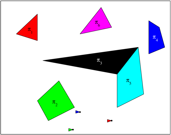
Figure 1: A polygonal environment, six regions of interest, and the initial deployment of three unicycle robots. Robot 1 is green, robot 2 is blue, and robot 3 is red; there is no relation between the robot and the region colors.

To provide a deployment strategy for Problem III.1, we will first combine various techniques from computational geometry, motion planning and model checking until we obtain a solution in the form of a sequence of tuples of smaller regions and feedback control laws in each of these regions. After this, we focus on the main contribution of the paper, namely finding a reduced set of communication (synchronization) moments among robots, while still guaranteeing the satisfaction of the specification. The main steps of the algorithmic approach for solving Problem III.1 are given in the following 3 subsections.

III-A Robot Abstraction

We first abstract the motion capabilities of each robot to a finite transition system. To this end, the environment is first partitioned into convex regions (cells) such that two adjacent cells exactly share a facet, and each region from $\Pi$ consists of a set of adjacent cells. Such a partition can be constructed by employing cell decomposition algorithms used in motion planning and computational geometry, e.g. one can use a constraint triangulation [21] or a polytopal partition [8]. Let us denote the set of partition elements by $C=\{c_{1},c_{2},\ldots,c_{|C|}\}$. For a clear understanding, Fig. 2 presents a triangular partition obtained for the environment from Fig. 1. We use a triangular partition for the case study presented throughout this paper, although our approach can be applied to any partition scheme.

Figure 2: Triangular partition consisting of 40 regions, corresponding to the environment from Fig. 1.

The second step is to reduce each unicycle with kinematics (1) to a fully-actuated point robot placed in unicycle’s reference point. We use the approach from [20], where a non-singular map relates the velocity $u$ of the reference point to the initial controls $w=[v,\omega]^{T}$. Note that $u$ can be conservatively bounded by a polyhedral set $U$, such that the resulted control $w$ is in $W$.

Definition III.1

The transition system abstracting the motion capabilities of unicycle $i$, $i=1,\ldots,n$ has the form $T_{i}=(Q_{i},q_{0i},\rightarrow_{i},\Pi\cup\{\emptyset\},\rho)$, where:

• $Q_{i}=C$, i.e. the set of states is given by the cells from partition;

• The initial state $q_{0i}\in C$ is the cell where the reference point of unicycle $i$ is initially deployed;

• The transition relation $\rightarrow_{i}\in C\times C$ is created as follows:

  • $(c_{i},c_{i})\in\rightarrow_{i}$ if we can design a feedback control law making cell $c_{i}$ invariant with respect to the trajectories of the reference point of unicycle $i$, and

  • $(c_{i},c_{j})\in\rightarrow_{i}$, $i\neq j$ if $c_{i}$ and $c_{j}$ are adjacent and we can design a feedback control law such that the reference point of unicycle $i$ leaves cell $c_{i}$ in finite time, by crossing the common facet of $c_{i}$ and $c_{j}$;

• $\Pi$ labels the set of regions of interest, and symbol $\emptyset$ corresponds to the space not covered by any region of interest;

• The observation map $\rho$ associates each cell from the partition with the corresponding proposition from $\Pi$, or with the symbol $\emptyset$.

Considering the unicycles reduced to their reference point, the construction of the continuous controllers corresponding to the transition relation from Definition III.1 is done by using results for facet reachability and invariance in polytopes [21]. We just mention that designing such feedback control laws reduces to solving a set of linear programming problems in every cell from partition, where the constraints result from the control bounds $U$ and the considered adjacent cells. Also, since the reference point is fully-actuated and the control bounds $U$ include the origin, we obtain a transition between every adjacent cells, as well as a self-loop in every state of $T_{i}$. Therefore, a run of $T_{i}$ can be implemented by unicycle $i$ by imposing specific control laws for the reference point in the visited cells, and by mapping these controls to $w$. We note that, since the unicycles are identical, the only difference between transition systems $T_{i}$ is given by their initial states.

Case study revisited: The partition from Fig. 2 enables us to construct a transition system with 40 states corresponding to each robot, where the transitions are based on adjacency relation between cells from environment, and the observations are given by the satisfied region. Fig. 3 illustrates some vector fields obtained from driving-to-facet control problems and from invariance controlled design, as well as the corresponding transitions from system $T_{i}$.

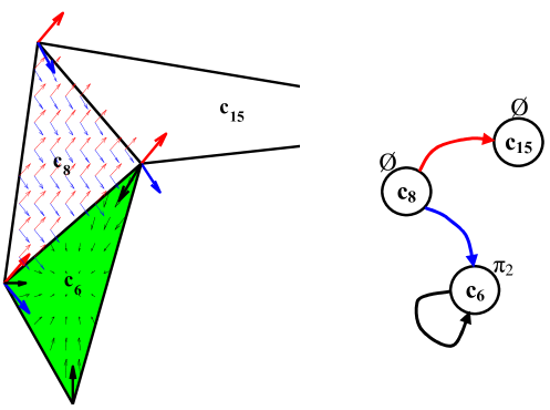
Figure 3: Left: vector fields driving any initial state from cell $c_{8}$ to a neighbor (blue and red colors), and vector field making $c_{6}$ invariant (black). Right: transitions from $T_{i}$ are colored in accordance with the colors of the created vector fields. Observation given by map $\rho$ is placed near each state.

III-B Satisfying Behavior of the Team

In this part of the solution, we use ideas from [27, 26] to find a run (for the whole team) satisfying the formula $\phi$. The $n$ transition systems $T_{i}$ are combined into a global one, $T_{G}$, capturing the synchronized motion of the team (synchronized in the sense that robots change at the same time the occupied cells from partition, or states from $T_{i}$). Then, by using model checking inspired techniques as mentioned in Sec. II, we find a run for the whole team, in the form of a prefix-suffix sequence of tuples.

Definition III.2

The transition system $T_{G}=(Q_{G},q_{G0},\rightarrow_{G},\Pi,\rho_{G})$ capturing the behavior of the group of $n$ robots is defined as the synchronous product of all $T_{i}$’s, $i=1,\ldots,n$:

• $Q_{G}=Q_{1}\times\ldots\times Q_{n}$,

• $q_{G0}=(q_{01},\ldots,q_{0n})$,

• $\rightarrow_{G}\subset Q_{G}\times Q_{G}$ is defined by $\left((q_{1},\ldots,q_{n}),(q^{\prime}_{1},\ldots,q^{\prime}_{n})\right)\in\rightarrow_{G}$ if and only if $(q_{i},q^{\prime}_{i})\in\rightarrow_{i}$, $i=1,\ldots,n$,

• $\Pi$ is the observation set,

• $\rho_{G}:Q_{G}\rightarrow 2^{\Pi}$ is defined by $\rho_{G}\left((q_{1},\ldots,q_{n})\right)=\cup_{i=1}^{n}\{\rho(q_{i})\}$.

We now find a run $R$ of $T_{G}$ such that the generated word $\rho_{G}(R)$ satisfies $\phi$. For this, we use the tool from [8], and we impose the optimality criterion that during the prefix and one iteration of the suffix, the total number of movements between partition cells is minimized. This is accomplished by adding weights to transitions of $T_{G}$, where the weight of a transition equals the number of robots that change their state from $T_{i}$. These weight are inherited when taking the product of $T_{G}$ with $B_{\phi}$. This optimality criterion minimizes the memory used on robots for storing motion controllers (feedback control laws driving robots from one cell to an adjacent one).

In [27, 26], such a global run was projected to individual runs of robots. Then, the robots can be controlled by the affine feedback controllers that map to unicycle controls from Sec. III-A. In deployment, when the team makes a transition from one tuple of the run to the next, the robots must synchronize (communicate) with each other and wait until every member finishes the previous transition. The synchronization will occur on the boundaries of the cells when crossing from a cell to another.

Remark III.1

Since the robots are identical, the number of states from $T_{G}$ can be reduced by designing a bisimilar (equivalent) transition system (the quotient induced by robot permutations) [27]. Thus, the computation complexity of finding a run $R$ is manageable even for large teams.

Case study revisited: For the above introduced example (Fig. 1 and 2, and specification (2)), we obtain a team run $R=\textrm{prefix, suffix, suffix},\ldots$, with 7 states in prefix and 8 states in suffix, as shown in Eqn. (3).

$$\begin{split}\textrm{prefix}=&\left(\begin{array}[]{c}c_{7}\\ c_{4}\\ c_{28}\end{array}\right)\,\left(\begin{array}[]{c}c_{2}\\ c_{3}\\ c_{28}\end{array}\right)\,\left(\begin{array}[]{c}c_{1}\\ c_{6}\\ c_{28}\end{array}\right)\,\left(\begin{array}[]{c}c_{10}\\ c_{8}\\ c_{28}\end{array}\right)\,\\ &\left(\begin{array}[]{c}c_{9}\\ c_{17}\\ c_{25}\end{array}\right)\,\left(\begin{array}[]{c}c_{18}\\ c_{11}\\ c_{26}\end{array}\right)\,\left(\begin{array}[]{c}c_{16}\\ c_{11}\\ c_{24}\end{array}\right)\,\,\,\\ \textrm{suffix}=&\left(\begin{array}[]{c}c_{31}\\ c_{12}\\ c_{38}\end{array}\right)\,\left(\begin{array}[]{c}c_{31}\\ c_{11}\\ c_{38}\end{array}\right)\,\left(\begin{array}[]{c}c_{31}\\ c_{17}\\ c_{24}\end{array}\right)\,\left(\begin{array}[]{c}c_{31}\\ c_{8}\\ c_{27}\end{array}\right)\,\\ &\left(\begin{array}[]{c}c_{31}\\ c_{6}\\ c_{20}\end{array}\right)\,\left(\begin{array}[]{c}c_{31}\\ c_{8}\\ c_{27}\end{array}\right)\,\left(\begin{array}[]{c}c_{31}\\ c_{17}\\ c_{27}\end{array}\right)\,\left(\begin{array}[]{c}c_{31}\\ c_{11}\\ c_{24}\end{array}\right)\end{split}$$ (3)

Run $R$ means that the robots start from their initial cells, and the first to robots evolve to cells $c_{2}$ and $c_{3}$ respectively. The synchronization imposed by the construction of $T_{G}$ and used in [27, 26] would require that the first two robots cross from $c_{7}$ to $c_{2}$ and from $c_{4}$ to $c_{3}$ synchronously (at exactly the same time), and so on. By construction, the word generated by $R$ over the set of propositions $\Pi$, $\rho_{G}(R)$, satisfies formula $\phi$ from Eqn. (2). However, the mentioned synchronizations are disadvantageous, because they require a lot of communication and waiting, and they imply many discontinuities is the control input of each robot (due to the frequent stops at the facets of traversed cell). Intuitively, one can observe that synchronizations along prefix of $R$ for example do not contribute to the satisfaction of the formula, nor they would lead to its violation, because the robots just head towards some regions they have to visit.

As evident from the case study, deployment strategies for a satisfying run $R$ as proposed in [27, 26] require a significant amount of synchronization (and thus communication) among the team. In this paper, rather than synchronizing robots for each transition in $R$, we aim in finding a reduced set of transitions along $R$ that require synchronization. This problem is formalized in Sec. III-C. Its solution is given in Sec. IV, in the form of an algorithmic procedure returning a reduced number of necessary synchronization moments along $R$, together with deployment strategies for robots. We note that in [26], we developed an algorithmic tool that tests if unsynchronized motion of the team can lead to a violation of the formula. If the answer is yes (such is the case for the case study considered in this paper), then synchronization required in [26] cannot be reduced. Therefore, the solution to the problem formulated in Sec. III-C constitutes a significant improvement over [26].

III-C Minimizing Communication

Problem III.2

Given a run $R$ of $T_{G}$ that satisfies the LTL specification $\phi$, find a team control and communication strategy that requires a reduced number of inter-robot synchronizations than in the synchronization-based deployment, while at the same time guaranteeing that the produced motion of the team satisfies $\phi$.

Central to our approach to Problem III.2 is an algorithm that takes as input the satisfying run $R=R(1)R(2)R(3)\ldots$ and returns a reduced number of necessary synchronization moments, where the $i^{\rm th}$ moment along R is defined as the index $i$ corresponding to $R(i)$. Motivated by the fact that synchronization by stopping and waiting at region boundaries is not always necessary to produce a desired tuple, we consider two types of synchronizations: in a weak synchronization, a certain tuple is generated because there exists an instant of time at which the robots are in the corresponding cells; a strong synchronization ensures that a sequence of two successive tuples from $R$ is observed. Note that a strong synchronization at each moment in $R$ is exactly the stop and wait strategy from [27, 26]. Since the run is given in the prefix-suffix form, our algorithmic framework will return a finite set of moments that require synchronization, as well as the type for each synchronization moment.

IV SOLUTION TO PROBLEM III.2

This section provides a solution to Problem III.2. We first construct an algorithmic procedure for finding a set of necessary synchronization moments (Sec. IV-A - IV-C), and then we present a communication strategy guaranteeing that the synchronization moments are satisfied (Sec. IV-D).

Without loss of generality, we assume that run $R=R(1)R(2)R(3)\ldots$ is in the prefix-suffix form (see Sec. II). Assume that the prefix has length $k-1$ and the suffix has length $l-k+1$, with $R(j)=\left(c^{1}_{j},c^{2}_{j},\ldots,c^{n}_{j}\right)^{T}$, for $j=1,\ldots,l$ (and $R(l+1)=R(k)$, $R(l+2)=R(k+1)$, $\ldots$). For avoiding supplementary notations implying repetitions of the suffix, we assume that whenever an index along $R$ exceeds $l$, that index is automatically mapped to the set $\{k,\ldots,l\}$, i.e. if $j=l$, then index $j+1$ is replaced with $k$, and so on. For an easier understanding, we use superscripts for identifying a robot and subscripts for indexing the cells.

For any robot $i=1,\ldots,n$ and for any moment $j=1,\ldots,l-1$, cells $c^{i}_{j}$ and $c^{i}_{j+1}$ are either adjacent or identical, and the same is true for cells $c^{i}_{l}$ and $c^{i}_{k}$. Recall that from the abstraction process of continuous robot trajectories, $R$ does not contain any successive and finite repetition of a $n$-tuple.

IV-A Finding Synchronization Moments

The idea of constructing a solution to Problem III.2 is to start with no synchronization moments, and iteratively test if the formula can be violated and update the set of synchronization moments and their type.

Let $S\subseteq\{1,\ldots,l\}$ be an arbitrary set of synchronization moments, and let us impose the type of each synchronization moment by creating a map $\tau:S\rightarrow\{weak,strong\}$, where $\tau(j)=weak$ means a weak synchronization at position $j$, and $\tau(j)=strong$ means a strong synchronization at position $j$, $\forall j\in S$.

As mentioned in Sec. III-C, a weak synchronization at moment $j$ along run $R$ means that the tuple $R(j)$ is reached by the robots, i.e., there is a moment when the robots are in cells $c^{1}_{j},\,c^{2}_{j},\ldots,c^{n}_{j}$, respectively. A strong synchronization at moment $j$ along run $R$ means that there is a weak synchronization at $j$, and additionally the robots synchronously enter the next tuple ($R(j+1)$). In other words, all moving robots $i$ cross from cells $c^{i}_{j}$ to cells $c^{i}_{j+1}$ at the same time.

One can observe that a strong synchronization at position $j$ is not equivalent to two weak synchronizations at $j$ and $j+1$. The strong synchronization guarantees that in the generated team run the tuple $R(j)$ is immediately followed by the tuple $R(j+1)$. However, the weak moments guarantee that the $R(j)$ and $R(j+1)$ tuples are generated, but there may appear different tuples between them. It can be noted that a weak synchronization at moment $j$ is equivalent with a strong one at the same moment if and only if $j=k$ and the suffix of $R$ has length 1 ($k=l$).

For testing the correctness of a set of synchronization moments, we developed a procedure $test\_feasibility_{\phi}(R,S,\tau)$, which takes as inputs the formula $\phi$, the run $R$, a set $S$ of synchronization moments and a map $\tau$. The returned output is either “feasible” (set $S$ with map $\tau$ guarantees the satisfaction of the formula, no matter how the robots move in between synchronization moments) or “not feasible” (it is possible to violate the formula by imposing just the moments from $S$ with type $\tau$). We postpone the details on $test\_feasibility_{\phi}(R,S,\tau)$ until Sec. IV-B.

We use Algorithm 1 for obtaining a solution to Problem III.2, in the form of a set $S$ of synchronization moments and a map $\tau$. The intuition behind this algorithm is to start with no synchronization moment ($S=\emptyset$) and increase $S$ until we obtain a feasible set together with a corresponding map $\tau$. We show the correctness of the solution given by Algorithm 1 in Sec. IV-C, together with more informal explanations on the provided pseudo-code.

Algorithm 1 Solution to Problem III.2

Inputs: Run $R$, formula $\phi$
Outputs: Set $S$, map $\tau$

1:  for $synch\_type\in\{weak,strong\}$ do

2:     $S=\emptyset$, $\tau$ undefined

3:     $lower_{bound}=1$, $moment=l$

4:     while $moment\geq lower_{bound}$ do

5:        if $test\_feasibility_{\phi}(R,S,\tau)$ = “feasible” then

6:           Return set $S$ and map $\tau$

7:        end if

8:        $S_{temp}=S\cup\{moment,moment+1,\ldots,l\}$

9:        $\tau_{temp}(i)=\tau(i),\,\forall i\in S$

10:        $\tau_{temp}(i)=synch\_type,\,\forall i\in\{moment+1,\ldots,l\}$

11:        for $\tau_{temp}(moment)\in\{weak,strong\}$ do

12:           if $test\_feasibility_{\phi}(R,S_{temp},\tau_{temp})$ = “feasible” then

13:              $S:=S\cup\{moment\}$

14:              $\tau(moment)=\tau_{temp}(moment)$

15:              $lower_{bound}=moment$

16:              $moment=l$

17:              Break “for” loop on $\tau_{temp}$

18:           else

19:              $moment:=moment-1$

20:           end if

21:        end for

22:     end while

23:  end for

Remark IV.1 (Complexity)

Algorithm 1 is guaranteed to finish, because in the worst case it returns the set $S=\{1,\ldots,l\}$, meaning that strong synchronizations are needed at every moment (see Sec. IV-C). The worst case complexity requires $3l(l+3)/2$ iterations of the test_feasibility procedure.

Remark IV.2 (Optimality)

Algorithm 1 can be tailored such that it returns an optimal solution (with respect to a cost defined by weighting different synchronization moments). This can be done by first constructing all possible pairs $S,\tau$ (there are $3^{l}$ such pairs). Then, these pairs should be ordered according to their associated cost. Finally, the pairs should be tested (in the found order) against the test_feasibility procedure, until a feasible response is obtained. Of course, the worst case would require $3^{l}$ iterations of test_feasibility (when the only solution is $S=\{1,\ldots,l\}$ and strong synchronization at every moment).

IV-B Testing a Set of Synchronization Moments

Procedure $test\_feasibility_{\phi}(R,S,\tau)$ follows several main steps:

1. It produces an automaton $A_{R,S,\tau}$ generating all the infinite words (sequences of observed propositions) that can result while the robots evolve and obey synchronization moments from $S$ (this automaton has the form of a Büchi automaton with an observation map);

2. If necessary, $A_{R,S,\tau}$ is transformed into a standard (degeneralized) form;

3. The product automaton between $A_{R,S,\tau}$ and the Büchi corresponding to negated LTL formula ($\mathcal{B}_{\neg\phi}$) is computed and its language is checked for emptiness;

4. If the language is empty, the procedure returns “feasible” and otherwise it returns “not feasible”.

For step (i), the run $R$ is projected to $n$ individual runs, each corresponding to a specific robot. In each of these individual runs, we collapse the finite successive repetitions of identical states (cells) into a single occurrence (such repetitions mean that the individual robot stays inside a cell). Let us denote the resulted runs by $R^{i}=q_{1}^{i}\,q_{2}^{i}\ldots\left[q_{k_{i}}^{i}\ldots q_{l_{i}}^{i}\right]\ldots$, where prefix has length $k_{i}-1$ ($k_{i}\leq k$) and suffix has length $l_{i}-k_{i}+1$ ($l_{i}\leq l$), $i=1,\ldots,n$. Together with individual projections and collapsing, we construct a set of maps $\beta_{i}:\{1,2,\ldots,l\}\rightarrow\{1,2,\ldots,l_{i}\}$, $i=1,\ldots,n$, mapping each index from run $R$ to the corresponding index from the individual run $R_{i}$ (e.g. $\beta_{i}(j)=\beta_{i}(j+1)$ if we have the same $i^{\rm th}$ element in tuples $R(j)$ and $R(j+1)$).

Next, we obtain a generalized Büchi automaton $A_{R,S,\tau}$ (see Def. II.2) whose runs are the possible sequences of tuples of cells visited during the team evolution. Thus, the language of $A_{R,S,\tau}$ contains all possible sequences of elements from $2^{\Pi}$ observed during the team movement. Each robot moves without synchronizing with the others, except for the moments from set $S$ with type $\tau$.

Definition IV.1

The automaton $A_{R,S,\tau}$ is defined as $A_{R,S,\tau}=(Q_{A},q_{A_{0}},\rightarrow_{A},F_{A},\Pi,\rho)$, where:

• $Q_{A}=\{q_{1}^{1},q_{2}^{1},\ldots,q_{l_{1}}^{1}\}\times\{q_{1}^{2},q_{2}^{2},\ldots,q_{l_{2}}^{2}\}\times\ldots\times\{q_{1}^{n},q_{2}^{n},\ldots,q_{l_{n}}^{n}\}$ is the set of states,

• $q_{A_{0}}=(q_{1}^{1},q_{1}^{2},\ldots,q_{1}^{n})$ is the initial state,

• $\rightarrow_{A}:Q_{A}\rightarrow 2^{Q_{A}}$ is the transition relation,

• $F_{A}\subset 2^{Q_{A}}$ is the set of sets of final states,

• $\Pi$ is the observation set,

• $\rho_{A}:Q_{A}\rightarrow 2^{\Pi}$ is the observation map, $\rho_{A}(q_{1},q_{2},\ldots,q_{n})=\cup_{i=1}^{n}\{\rho(q_{i})\}$.

The transition relation $\rightarrow_{A}$ is defined as follows: $\forall q,q^{\prime}\in Q_{A}$, with $q=(q_{j_{1}}^{1},q_{j_{2}}^{2},\ldots,q_{j_{n}}^{n})$ and $q^{\prime}=({q^{\prime}}_{j_{1}}^{1},{q^{\prime}}_{j_{2}}^{2},\ldots,{q^{\prime}}_{j_{n}}^{n})$, $\left(q,q^{\prime}\right)\in\rightarrow_{A}$ if and only if the following rules are simultaneously satisfied:

1. $q=q^{\prime}$ if and only if $j_{i}=k_{i}$ and $k_{i}=l_{i}$, $i=1,\ldots,n$;

2. ${q^{\prime}}_{j}^{i}\in\{q_{j}^{i},q_{j+1}^{i}\}$ if $j\in\{1,2,\ldots,l_{i}-1\}$, and ${q^{\prime}}_{j}^{i}\in\{q_{l_{i}}^{i},q_{k_{i}}^{i}\}$ if $j=l_{i}$, $i=1,2,\ldots,n$;

3. if $\exists s\in S$ such that $j_{i}=\beta_{i}(s)$ for $i\in I\subseteq\{1,\ldots,n\}$, where $I$ is the largest possible subset of robots satisfying this requirement, then:

   1. if $I\neq\{1,\ldots,n\}$, then ${q^{\prime}}_{j_{i}}^{i}=q_{j_{i}}^{i}$, $\forall i\in I$;

   2. if $I=\{1,\ldots,n\}$ and $\tau(s)=strong$, then ${q^{\prime}}_{j_{i}}^{i}=q_{\beta_{i}(s+1)}^{i}$, $\forall i\in I$.

Informally, requirements (a) and (b) capture a global progress/movement along individual runs of robots, by also capturing the possible situations when some robots advance “slower” (from the point of view that it takes more time for them to reach the next cell from partition). Requirement (c) restricts transitions by assuming that the agents satisfy all synchronization moments from $S$ with type given by $\tau$.

Before detailing the construction of $F_{A}$, we say that we consider as a generated word of $A_{R,S,\tau}$ any trajectory that infinitely often visits all sets of states from $F_{A}$. This definition of generated words is exactly the definition of accepting words of generalized Büchi automata. Moreover, $A_{R,S,\tau}$ has a structure similar to a Büchi automaton, which has final sets of states that are infinitely often encountered along an accepted run.

The set of sets of final states of $A_{R,S,\tau}$ ($F_{A}$) is created by using Algorithm 2. The construction from Algorithm 2 matches the purpose of generated runs of $A_{R,S,\tau}$, in the sense that any run contains infinitely many revisits to tuples from suffix of $R$ where synchronization is imposed. More details on the construction of $A_{R,S,\tau}$ are given in Sec. IV-C.

Algorithm 2 Set of final sets of automaton $A_{R,S,\tau}$

1:  $S_{suffix}=S\cap\{k,\ldots,l\}$

2:  if $S_{suffix}=\emptyset$ then

3:     $F_{A}=\{q_{k_{1}}^{1},\ldots,q_{l_{1}}^{1}\}\times\{q_{k_{2}}^{2},\ldots,q_{l_{2}}^{2}\}\times\ldots\times\{q_{k_{n}}^{n},\ldots,q_{l_{n}}^{n}\}$

4:  else

5:     Assume $S_{suffix}=\{s_{1},s_{2},\ldots,s_{|S_{suffix}|}\}$

6:     $F_{A}=\{F_{1},F_{2},\ldots,F_{|S_{suffix}|}\}$

7:     for $j=1,2,\ldots,|S_{suffix}|$ do

8:        $F_{j}=\{q_{\beta_{1}(s_{j})}^{1},q_{\beta_{2}(s_{j})}^{2},\ldots,q_{\beta_{n}(s_{j})}^{n}\}$

9:     end for

10:  end if

Once $A_{R,S,\tau}$ is constructed, we have to check if there exists a generated word of $A_{R,S,\tau}$ that violates the LTL formula (by satisfying the negation of the formula). As mentioned at the beginning of this section, this basically implies checking for emptiness the language of a product between $A_{R,S,\tau}$ and $\mathcal{B}_{\neg\phi}$ (steps (ii)-(iv)).

Similar to finding a run as mentioned in Sec. II, this emptiness checking can be done by using available software tools for normal (degeneralized) Büchi automata. In case that $F_{A}$ contains more than one set, $A_{R,S,\tau}$ has the structure of a generalized Büchi automata. If this is the case, we first convert $A_{R,S,\tau}$ into a degeneralized form (as mentioned in Sec. II), and then we construct the product with $\mathcal{B}_{\neg\phi}$. The construction of this product is similar to the one constructed between transition systems and Büchi automata [8]. The only difference is that the set of final states of product equals the cartesian product between final states of (degeneralized) $A_{R,S,\tau}$ and the final states of Büchi.

Example of constructing $A_{R,S,\tau}$: We include here a simple example, solely for the purpose of understanding the construction of $A_{R,S,\tau}$. Therefore, we do not define an environment, nor we impose an LTL formula. Consider a team of 2 robots and the following run $R$:

$$R=\left(\begin{array}[]{c}c_{5}\\ c_{6}\end{array}\right)\,\left[\left(\begin{array}[]{c}c_{1}\\ c_{2}\end{array}\right)\,\left(\begin{array}[]{c}c_{7}\\ c_{2}\end{array}\right)\,\left(\begin{array}[]{c}c_{3}\\ c_{4}\end{array}\right)\,\right]\,\ldots$$ (4)

$R$ has a prefix of length 1, and a suffix of length 3 (the suffix is represented between square brackets).

First, assume an empty set of synchronization moments, $S=\emptyset$. By projecting $R$ to individual runs and collapsing successive identical states, we obtain: $R^{1}=q_{1}^{1}\left[q_{2}^{1}q_{3}^{1}q_{4}^{1}\right]$ and $R^{2}=q_{1}^{2}\left[q_{2}^{2}q_{3}^{2}\right]$, where $q_{1}^{1}=c_{5}$, $q_{2}^{1}=c_{1}$, $q_{3}^{1}=c_{7}$, $q_{4}^{1}=c_{3}$, $q_{1}^{2}=c_{6}$, $q_{2}^{2}=c_{2}$, $q_{3}^{2}=c_{4}$. The obtained automaton $A_{R,\emptyset,\emptyset}$ is given in Fig. 4(a), where the initial state is $(q_{1}^{1},q_{1}^{2})$. This automaton is already in degeneralized form (it has a single set of final states), because $S$ does not contain synchronization moments along suffix. Also, note that once the final set of $A_{R,\emptyset,\emptyset}$ is reached, it is never left. This corresponds to the fact that both robots reach and follow their suffixes (independently), and any possible observed sequence during the movement corresponds to a word generated by $A_{R,\emptyset,\emptyset}$.

Now, assume a set $S=\{2,4\}$, with $\tau(2)=strong$ and $\tau(4)=weak$. This means there is a strong synchronization at the beginning of every iteration of suffix of $R$ (state $(c_{1},c_{2})$) and a weak synchronization at the end (state $(c_{3},c_{4})$). The automaton $A_{R,S,\tau}$ created as described in this subsection is given in Fig. 4(b). This automaton has the same set of states and observations as $A_{R,\emptyset,\emptyset}$, but the set of transitions is reduced because of synchronization rules. $A_{R,S,\tau}$ is in generalized form, because it has 2 sets of final states ($F_{1}=(q_{2}^{1},q_{2}^{2})$ and $F_{2}=(q_{4}^{1},q_{3}^{2})$). They gray states become unreachable because the reduced transitions of $A_{R,S,\tau}$. Note that any word generated by $A_{R,S,\tau}$ infinitely often visits state $(q_{2}^{1},q_{2}^{2})$ (which corresponds to the first synchronization moment from $S$) and state $(q_{4}^{1},q_{3}^{2})$ (corresponding to the second synchronization moment from $S$). Also, there is only one outgoing transition from $(q_{2}^{1},q_{2}^{2})$, in accordance with the strong synchronization in this state. It should be clear why in this case we have 2 sets of final states: if we had a single set, containing both $(q_{2}^{1},q_{2}^{2})$ and $(q_{4}^{1},q_{3}^{2})$, then $A_{R,S,\tau}$ would have been accepting words like $(q_{1}^{1},q_{1}^{2})\,\left[(q_{2}^{1},q_{2}^{2})\,(q_{3}^{1},q_{2}^{2})\,(q_{4}^{1},q_{2}^{2})\right]\ldots$. However, such a word would correspond to a spurious (impossible) movement of robots, because state $(q_{4}^{1},q_{3}^{2})$ would never be visited, although it corresponds to a synchronization moment.

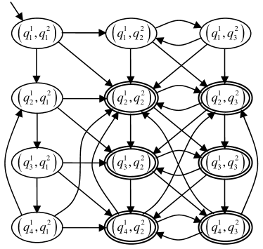
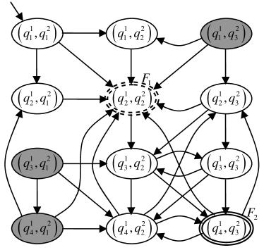
(a)	(b)

Figure 4: Examples of two automata constructed as described in Sec. IV-B, from run $R$ from Eqn. (4): (a) $A_{R,\emptyset,\emptyset}$; (b) $A_{R,\{2,4\},\tau}$, with $\tau(2)=strong$ and $\tau(4)=weak$. Final states are double encircled, with different line types corresponding to different final sets, and the gray states are not reachable.

IV-C Correctness of Solution to Problem III.2

Theorem IV.1

Any solution returned by Algorithm 1 is a feasible solution to Problem III.2, and Algorithm 1 returns a solution in a finite number of steps.

Proof:

The correctness of Algorithm 1 and of the “test_feasibility” procedure results by the construction we performed in this section, as detailed below.

Correctness of “test_feasibility” procedure: We first prove that the “test_feasibility” procedure cannot yield a “feasible” output if the inputs $S$ and $\tau$ can produce a violation of the formula. This comes from the requirements of the transition relation $\rightarrow_{A}$ and from the construction of $F_{A}$. Requirement (a) from definition of $\rightarrow_{A}$ means that $A_{R,S,\tau}$ does not self-loops, except for the case when all individual runs have suffixes of length 1 (in this case a self-loop exists for reiterating the suffix). Requirement (b) results from the fact that every robot $i$ follows its individual run $R^{i}$ and iterates the suffix; the fact that there is no synchronization (a moving robot might not change its current cell, while others advance along their individual runs) is captured by the possibility of having $q_{j}=q^{\prime}_{j}$ for some robots. Thus, requirements (a) and (b) capture a global progress/movement along individual runs of robots, by enforcing iterations of individual suffixes. If we ignore requirement (c), and we assume that $F_{A}$ is just a single set constructed as in line 3 of Algorithm 2, $A_{R,S,\tau}$ can generate any possible run resulted while robots evolve without any synchronization (set $S$ and map $\tau$ were not yet used). Thus, if “test_feasibility” returns a “feasible” answer, it means that even the unsynchronized movement is feasible, so the motion restricted by $(S,\tau)$ would definitely imply a satisfaction of $\phi$. However, such an approach would be very conservative, because it does not restrict the possible generated runs of $A_{R,S,\tau}$ based on $S$ and $\tau$.

Conservativeness reduction of $\rightarrow_{A}$: Requirement (c) restricts transitions based on synchronization moments and their type. Thus, (c.(1)) guarantees that if one or more robots arrived at a synchronization moment, then they will not continue following the individual runs (by changing their states) unless all other robots arrived at that synchronization moment. This way, (c.(1)) captures the fact that the weak synchronization moments and the first part of the strong ones (visiting a certain tuple) are satisfied. Requirement (c.(2)) ensures that a tuple of cells corresponding to a strong synchronization moment is synchronously left by all robots that have to move at that index (the moving robots synchronously go to the next state from their individual run, while for other robots $\beta_{i}(s+1)$ implies remaining in the same state/cell). The reduced set of transitions of $A_{R,S,\tau}$ captures the satisfaction of all synchronization moments, and includes all possible unsynchronized (independent) movements of robots between synchronization moments. Therefore, the correctness of “test_feasibility” is not affected, while its conservativeness is reduced.

Construction of $F_{A}$: If there is no synchronization moment in the suffix of $R$, then $F_{A}$ contains only one set, equal to the cartesian product of the sets of states composing the suffixes of individual runs $R^{i}$, $i=1,\ldots,n$ (line 3 in Algorithm 2). This is because no synchronization moment in suffix of $R$ means no synchronization moments in suffixes of individual runs. Therefore, the robots independently follow their suffixes and any $n$-tuple from set $F_{A}$ can be infinitely often observed during the team evolution. In this case $A_{R,S,\tau}$ is still too conservative, because it can generate many runs that cannot result from the actual movement of robots (e.g. infinite surveillance of just two states from $F_{A}$).

The set of accepted runs is drastically reduced if there are $x$ synchronization moments in suffix of $R$ (and also in individual suffixes). In this case, $F_{A}$ will contain $x$ sets (in Algorithm 2, $x=|S_{suffix}|$). Each of these sets contains just one tuple, which corresponds to one synchronization moment along individual suffixes. This construction comes from the following aspects: (i) due to synchronization moments along suffixes, we have additional information about some infinitely visited states, and considering $F_{A}$ as in line 3 of Algorithm 2 would be too conservative. (ii) If there are more synchronization moments along suffix, having a single set of final states that contains all the corresponding tuples would be again too conservative. This is because the transitions of $A_{R,S,\tau}$ might allow infinitely often revisits to just a single element of that set, and we might get spurious counterexamples when testing $A_{R,S,\tau}$ against the negation of LTL formula. (iii) In case of a strong synchronization moment $j$ along the suffix, adding two states (tuples corresponding to $R(j)$ and $R(j+1)$) in the corresponding element of $F_{A}$ would not bring any additional benefit than adding just $R(j)$ (as done in Algorithm 2). This is because requirement (c.(2)) implies that the only possible transition from state corresponding to $R(j)$ is to the state corresponding to $R(j+1)$. Therefore, construction of $F_{A}$ as in Algorithm 2 further reduces the conservativeness of $A_{R,S,\tau}$ by restricting its set of generated runs with respect to $S$ and $\tau$. $A_{R,S,\tau}$ still generates all possible sets of tuples that the team can follow while moments from $S$ with type $\tau$ are satisfied.

There is one more step in proving the correctness of “test_feasibility”, namely that there exists a pair $S,\tau$ for which “test_feasibility” returns a “feasible” output. This pair is $S=\{1,\ldots,l\}$ and $\tau(j)=strong$, $\forall j\in S$. Indeed, in this case every state of $A_{R,S,\tau}$ has only one outgoing transition, and the only run generated by $A_{R,S,\tau}$ is $R$. The word generated by $R$ satisfies formula $\phi$ (because $R$ was constructed by assuming it is strongly synchronized at every position). Therefore, the language of the product between the degeneralized $A_{R,S,\tau}$ and $\mathcal{B}_{\neg\phi}$ is empty, and “test_feasibility” returns “feasible”.

Correctness of Algorithm 1: We now prove that Algorithm 1 returns a feasible pair $(S,\tau)$ in a finite number of steps. First, we explain Algorithm 1 and we show that the worst case ($S=\{1,\ldots,l\}$ and $\tau(j)=strong$, $\forall j\in S$) is returned, if no other less restrictive pair $(S,\tau)$ was encountered.

Algorithm 1 starts with $S=\emptyset$ and $\tau$ undefined, and increases $S$ with at most one moment at every iteration of the “while” loop from line 4. For this, it goes from the last index in suffix of $R$ (moment $l$) towards the first one, and it constructs a temporary set of synchronization moments ($S_{temp}$). $S_{temp}$ includes all the moments from $S$ (initially none) and all indices after the current moment until $l$. All moments following the currently tested one are first assumed to be weakly synchronized, and if no solution is obtained, they will be assumed strong (line 10 and “for” loop starting on line 1). This is because we consider a strong synchronization more disadvantageous than a weak one, due to the waiting and communication at borders separating adjacent cells. The current moment is first tested with a weak synchronization, and if no feasible answer results, it is tested with strong synchronization (loop starting on line 11). If the current test (with $S_{temp}$ and $\tau_{temp}$) is feasible, we add to set $S$ only the current moment, with its current synchronization type stored in map $\tau$ (lines 13, 14). Then, on line 15 we update the lower bound for the current synchronization moment (it doesn’t make sense to go lower than the just found moment), and we start again the while loop on line 4 (from moment $l$ towards the lower bound). For each disjoint assignment of “synch_type” (“for” loop on line 1), the currently tested moment inside the “while” loop from line 4 is build on the feasible moments existing in $S$ and $\tau$ until that instant (those moments are included in $S_{temp}$ and $\tau_{temp}$ on lines 8, 9).

Once a feasible pair $S_{temp},\tau_{temp}$ is encountered, all future iterations from Algorithm 1) try to reduce the number of moments from $S_{temp}$ and relax their synchronization type. In the worst case the same pair will be returned: if no other feasible pair included in this one is found, after a number of iterations of the “while” loop the same pair is again encountered (but this time, the first element of the old/feasible $S_{temp}$ is already in $S$). Now, the second element from the old $S_{temp}$ (the first from the new $S_{temp}$) is added to $S$ and the “while” loop is again iterated, and so on. Thus, once a feasible pair is encountered, Algorithm 1 finishes in a finite number of steps.

For proving that a feasible pair $(S_{temp},\tau_{temp})$ is ever encountered, we show that, if no other feasible pair is found, the algorithm eventually tests the pair where $S_{temp}=\{1,\ldots,l\}$ and $\tau_{temp}(j)=strong$, $\forall j\in S_{temp}$ (this pair is deemed feasible by the “test_feasibility” procedure, as shown before). When $synch\_type=weak$ (first iteration of “for” loop on line 1), we iterate the “while” loop for $l$ times and we do not get any feasible result. For $synch\_type=strong$ we would get $S_{temp}=\{1,\ldots,l\}$ and $\tau_{temp}(j)=strong$, $\forall j\in S_{temp}$ after another $l$ iterations of the “while” loop. Even though we get a “feasible” answer from “test_feasibility”, we add just the first moment from $S_{temp}$ to $S$ (so $S=\{1\}$) and reiterate. This time, at the $(l-1)^{\rm th}$ iteration of the “while” loop we would get the same pair $(S_{temp},\tau_{temp})$ (when $moment=2$). Now, $S$ is updated to $S=\{1,2\}$ and the “while” loop is reiterated with $lower_{bound}=2$. Since each iteration of “while” loop includes 3 calls to the “test_feasibility” procedure, the total number of such calls is: $3\left(l\,+\,l+(l-1)+(l-2)+\ldots+1\right)=3l(l+3)/2$.

By using a similar reasoning as above, it can be easily shown that if there exists a set $S\subseteq\{1,\ldots,l\}$ and a map $\tau$ for which $test\_feasibility_{\phi}(R,S,\tau)$=“feasible”, then the pair $(S,\tau)$ will be encountered by Algorithm 1 if other feasible pair is not encountered before. This shows why Algorithm 1 does not necessarily find an optimal solution (with respect to a cost defined by weighting different synchronization moments): once a feasible pair $(S_{temp},\tau_{temp})$ is encountered, all future iterations test only subsets of $S_{temp}$, not other sets from $\{1,\ldots,l\}$.  

IV-D Communication and Control Strategy

We complete the solution to Problem III.2 by providing a deployment strategy such that the synchronization moments from set $S$ with type $\tau$ are correctly implemented. A weak synchronization at moment $j$ along $R$ is achieved by enforcing each robot $i$ to wait inside cell $c^{i}_{j}$ (and signal this to others) until it receives a similar signal from all other robots. A strong synchronization at moment $j$ is accomplished by first enforcing a weak synchronization at moment $j$, and then temporary stopping the robots for which $c^{i}_{j}\neq c^{i}_{j+1}$ just before leaving cell $c^{i}_{j}$ (and entering $c^{i}_{j+1}$).

Since we need individual strategies, we have to adapt the set $S$ and map $\tau$ to descriptions suitable for each robot $i$ that moves along its individual run $R^{i}$, $i=1,\ldots,n$. To solve this, for each robot $i$ we construct a queue memory $Q^{i}$, where each entry contains the index along $R^{i}$ when there should be enforced a synchronization, and the synchronization type. Alg. 3 creates these queue memories by adding $|S|$ entries, in the ascending order of moments from $S$.

Algorithm 3 Queue memory $Q^{i}$

1:  $Q^{i}=\emptyset$

2:  for all $s\in S$ do

3:     Assume that $S$ is sorted and states in $S$ are enumerated sequentially

4:     $moment=\beta_{i}(s)$

5:     $type=\tau(s)$

6:     Add entry $[moment,type]$ at the end of $Q^{i}$

7:  end for

Algorithm 4 Individual strategy for robot $i$

1:  $j=1$

2:  while TRUE do

3:     Read first entry $[moment,type]$ from $Q^{i}$

4:     Read second entry $[next\_moment,next\_type]$ from $Q^{i}$

5:     if $moment=j$ then

6:        while “ready” signals not received from all other robots do

7:           Broadcast a “ready to synchronize” signal

8:           Apply convergence controller inside current cell $q^{i}_{j}$ from run $R^{i}$

9:        end while

10:        if $next\_moment\neq j$ then

11:           Apply controller driving to the next cell $q^{i}_{j+1}$ until border between $q^{i}_{j}$ and $q^{i}_{j+1}$ is reached

12:        end if

13:        if $type=strong$ then

14:           while “ready” signals not received from all other robots do

15:              Broadcast a “ready to synchronize” signal

16:              if $next\_moment\neq j$ then

17:                 Stop robot

18:              else

19:                 Apply convergence controller inside current cell $q^{i}_{j}$

20:              end if

21:           end while

22:        end if

23:        if $j<k_{i}$ then

24:           Remove first entry from $Q^{i}$

25:        else

26:           Move first entry from $Q^{i}$ to the end of $Q^{i}$

27:        end if

28:        if $next\_moment\neq j$ then

29:           $j:=j+1$

30:        end if

31:     else

32:        if $q^{i}_{j}\neq q^{i}_{j+1}$ then

33:           Apply controller driving to the next cell $q^{i}_{j+1}$ until border between $q^{i}_{j}$ and $q^{i}_{j+1}$ is reached

34:           $j:=j+1$

35:        else

36:           Apply convergence controller inside current cell $q^{i}_{j}$

37:        end if

38:     end if

39:  end while

The queues $Q^{i}$ will be used by the robots in a FIFO manner, as in Alg. 4. Each robot follows the infinite run $R^{i}$, by applying correct feedback controllers and by synchronizing with other robots when required. After fulfilling a synchronization moment, the corresponding entry from $Q^{i}$ is removed or moved to the end, depending on the inclusion of the current moment in prefix or suffix. The current index in $R^{i}$ is incremented based on specific conditions, for correctly handling the situations when two or more synchronization moments from $S$ yield the same value through map $\beta_{i}$. Note that the robots not changing their cell when a strong synchronization moment is required still synchronize twice on that moment (for the weak and then the strong part), but they apply a convergence controller inside current cell.

V CASE STUDY REVISITED

This section concludes the case study illustrated throughout the paper, by applying the procedure described in Sec. IV to the run from Eqn. (3). We obtain only two weak synchronization moments, at indices 8 and 12 of run $R$ (first and fifth positions of every repetition of suffix). This makes sense, since the propositions satisfied by the team at the two synchronization moments are the two sets of regions ($\{\pi_{1},\,\pi_{4},\,\pi_{6}\}$ and $\{\pi_{2},\,\pi_{5}\}$) that are required to be visited for the satisfaction of the formula.

The individual runs of the robots are given in Eqn. (5), where the square brackets delimitate each suffix, and the two weak synchronization moments are marked in bold:

$$\begin{array}[]{l}R^{1}=c_{7}\,c_{2}\,c_{1}\,c_{10}\,c_{9}\,c_{18}\,c_{16}\,\left[{\bf c_{31}}\right]\,\left[{\bf c_{31}}\right]\ldots\\ R^{2}=c_{4}\,c_{3}\,c_{6}\,c_{8}\,c_{17}\,c_{11}\,\left[{\bf c_{12}}\,c_{11}\,c_{17}\,c_{8}\,{\bf c_{6}}\,c_{8}\,c_{17}\,c_{11}\right]\ldots\\ R^{3}=c_{28}\,c_{25}\,c_{26}\,c_{24}\,\left[{\bf c_{38}}\,c_{24}\,c_{27}\,{\bf c_{20}}\,c_{27}\,c_{24}\right]\ldots\end{array}$$ (5)

The control and communication protocol from Sec. IV-D points to the following deployment strategy for each robot: the robot moves along its individual run without any communication, until it encounters a required synchronization moment. Then, it broadcasts that it is in a “ready” mode for the synchronization moment, and it waits inside the current cell until it receives “ready” signals for the current moment from all other robots. After this, each robot evolves again individually (without any synchronization) until the next synchronization moment. Note that for the above example, once robot 1 reaches its suffix it keeps applying a convergence controller inside $c_{31}$ and broadcasting a “ready” signal (so that it does not induce waiting for other robots).

Some snapshots from the deployment (implemented according to Sec. IV-D) are shown in Fig. 5, where two repetitions of the suffix for each robot are included. A movie for the case study is available at http://hyness.bu.edu/~software/unicycles.mp4. For comparison, if we avoided solving Problem III.2 and instead used the deployment strategy from [26], we would get the team trajectory illustrated by the movie http://hyness.bu.edu/~software/unicycles-full-synch.mp4. In this movie, we can see that the motions of the robots are not as “smooth” as our proposed approach, and the iterations for each suffix require more time. Our approach is more suitable for real experiments as robots have less frequent stops at region borders.

(a)	(b)	(c)	(d)
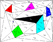
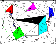
(e)	(f)	(g)	(h)

Figure 5: Several configurations reached during movement ((a)$\ldots$(g)), and traces of robots (h). (a) Robot 1 (green) heads to $c_{31}$, robot 2 (blue) heads to $c_{12}$, robot 3 (red) heads to $c_{38}$; (b) Robot 3 begins to wait for the first weak synchronization moment from suffix; (c) Robots 2 and 3 are waiting (by converging inside their regions); (d) First synchronization moment is accomplished, all robots continue normal movement; (e) Robot 3 begins waiting for the second synchronization moment; (f) Synchronization accomplished, robots 2 and 3 head back to $c_{12}$ and $c_{38}$ respectively; (g) Robot 3 begins waiting for the first synchronization moment from suffix, and when robot 2 reaches $c_{12}$ a new iteration of suffix begins.

Computation time: The most computationally intensive part of the solution to Problem III.1 is finding a run $R$ (as in Sec. III-A and III-B). For our case study, this took about 100 minutes on a medium performance computer. In contrast, the solution we proposed for Prob. III.2 (Sec. IV) took only 30 seconds. To generate a solution for Prob. III.2, 26 iterations of the test_feasibility procedure were performed until the set of synchronization moments was found.

VI ADDITIONAL EXAMPLE

This section briefly presents another example on the same environment as in Fig. 1, but considering two robots and the LTL formula:

$$\begin{split}\phi&=\{\neg(\pi_{3}\vee\pi_{5})U(\pi_{1}\wedge\pi_{2})\}\wedge\\ &\{\neg(\pi_{3}\vee\pi_{4}\vee\pi_{5})U(\pi_{4}\wedge\pi_{5})\}\wedge\{\diamondsuit\square(\pi_{3}\vee\pi_{6})\}\end{split}$$ (6)

The curly brackets are only inserted to logically delimitate the requirements: (i) black and cyan regions ($\pi_{3}$ and $\pi_{5}$) should be avoided until red and green regions are visited, and (ii) black region is avoided until blue and cyan regions are entered at the same time, and (iii) eventually either the black or the magenta region should be visited and never left after that.

By considering the robots initially deployed in regions $c_{1}$ and $c_{26}$ respectively, we obtained a run for the team with 12 tuples in prefix and one in suffix. Informally, first robot goes to red region and the second one to the green one, then the robots move toward blue and cyan regions, and after these regions are simultaneously entered, the second robot goes to the black region and converge there, while the first robot remains in the blue region.

By searching synchronization moments, we obtain only two such moments: a weak one, at the tuple when robots visit the red and green regions, and a strong one at the tuple before visiting the blue and cyan regions. The second synchronization moment guarantees that the blue and cyan regions are entered at the same time. These synchronization moments automatically found by our approach are natural at an insightful study of the requirement. The movement of the robots is depicted in the movie available at http://hyness.bu.edu/~software/unicycles-example2.mp4. In this movie one can observe both synchronization moments: (1) red robot arrives in the red region and it starts to converge there until the green robot visits the green region; (2) green robot arrives in cell $c_{40}$ and starts to converge there until red robot visit cell $c_{37}$ (this is the weak synchronization part of the strong moment), and then the robots move towards blue and cyan regions. Red robot stops at the border between $c_{37}$ and $c_{29}$ and waits until the green robot reaches the border between $c_{40}$ and $c_{21}$ - this ensures the strong part of the synchronization (simultaneously change occupied cells). After this, no other communication between robots is required.

VII CONCLUSIONS

We presented a fully automated framework for deploying a team of unicycles from a task specified as a linear temporal logic formula over some regions of interest. The approach consists of abstracting the motion capabilities of each robot into a finite state representation, using model checking tools to find a satisfying run, and mapping the solution to a communication and control strategy for each unicycle. The main contribution of the paper is the development of an algorithmic procedure that returns a reduced set of moments when the robots should communicate and synchronize, with the guarantee that the specification is satisfied. A secondary contribution is the integration of this algorithm as part of a fully automatic procedure for deployment of teams of unicycles from specifications given as LTL formulas over regions of interest in an environment. Future research direction includes extending this framework to probabilistic systems such as Markov Decision Processes (MDPs) or Partially Observable Markov Decision Processes (POMDPs), for satisfaction of probabilistic temporal logics, such as probabilistic LTL or probabilistic CTL.

References

- [1] S. M. LaValle, Planning Algorithms. Cambridge University Press, 2006, available at http://planning.cs.uiuc.edu.
- [2] S. Russell and P. Norvig, Artificial Intelligence: A Modern Approach, 2nd ed. Prentice Hall, 2003.
- [3] E. Rimon and D. E. Koditschek, “Exact robot navigation using artificial potential functions,” IEEE Transactions on Robotics and Automation, vol. 8, no. 5, pp. 501–518, 1992.
- [4] S. M. LaValle and J. J. Kuffner, “Randomized kinodynamic planning,” International Journal of Robotics Research, vol. 20, no. 5, pp. 378–400, 2001.
- [5] R. Tedrake, I. R. Manchester, M. M. Tobenkin, and J. W. Roberts, “LQR-trees: Feedback motion planning via sums of squares verification,” International Journal of Robotics Research, vol. 29, no. 8, pp. 1038–1052, 2010.
- [6] M. Antoniotti and B. Mishra, “Discrete event models + temporal logic = supervisory controller: Automatic synthesis of locomotion controllers,” in IEEE Int. Conf. on Robotics and Automation, Nagoya, Japan, 1995, pp. 1441–1446.
- [7] S. Karaman and E. Frazzoli, “Sampling-based motion planning with deterministic -calculus specifications,” in IEEE Conf. on Decision and Control, Shanghai, China, 2009, pp. 2222 – 2229.
- [8] M. Kloetzer and C. Belta, “A fully automated framework for control of linear systems from temporal logic specifications,” IEEE Transactions on Automatic Control, vol. 53, no. 1, pp. 287–297, 2008.
- [9] H. Kress-Gazit, G. Fainekos, and G. J. Pappas, “Where’s Waldo? Sensor-based temporal logic motion planning,” in IEEE Int. Conf. on Robotics and Automation, Rome, Italy, 2007, pp. 3116–3121.
- [10] S. G. Loizou and K. J. Kyriakopoulos, “Automatic synthesis of multiagent motion tasks based on LTL specifications,” in IEEE Conf. on Decision and Control, Paradise Island, Bahamas, 2004, pp. 153–158.
- [11] M. M. Quottrup, T. Bak, and R. Izadi-Zamanabadi, “Multi-robot motion planning: A timed automata approach,” in IEEE Int. Conf. on Robotics and Automation, New Orleans, LA, 2004, pp. 4417–4422.
- [12] T. Wongpiromsarn, U. Topcu, and R. M. Murray, “Receding horizon temporal logic planning for dynamical systems,” in IEEE Conf. on Decision and Control, Shanghai, China, 2009, pp. 5997–6004.
- [13] C. Baier, J.-P. Katoen, and K. G. Larsen, Principles of Model Checking. MIT Press, 2008.
- [14] E. M. Clarke, D. Peled, and O. Grumberg, Model checking. MIT Press, 1999.
- [15] J. Hopcroft, R. Motwani, and J. D. Ullman, Introduction to Automata Theory, Languages, and Computation. Addison Wesley, 2007.
- [16] R. Alur, T. A. Henzinger, G. Lafferriere, and G. J. Pappas, “Discrete abstractions of hybrid systems,” Proceedings of the IEEE, vol. 88, pp. 971–984, 2000.
- [17] C. Belta and L. Habets, “Controlling a class of nonlinear systems on rectangles,” IEEE Transactions on Automatic Control, vol. 51, no. 11, pp. 1749–1759, 2006.
- [18] R. Burridge, A. Rizzi, and D. Koditschek, “Sequential composition of dynamically dexterous robot behaviors,” The International Journal of Robotics Research, vol. 18, no. 6, p. 534, 1999.
- [19] D. Conner, H. Choset, and A. Rizzi, “Integrated planning and control for convex-bodied nonholonomic systems using local feedback control policies,” Proceedings of robotics: Science and systems II, 2006.
- [20] J. Desai, J. Ostrowski, and V. Kumar, “Controlling formations of multiple mobile robots,” in Proc. IEEE Int. Conf. Robot. Automat., Leuven, Belgium, 1998.
- [21] L. Habets, P. Collins, and J. van Schuppen, “Reachability and control synthesis for piecewise-affine hybrid systems on simplices,” IEEE Transactions on Automatic Control, vol. 51, pp. 938–948, 2006.
- [22] R. Milner, Communication and concurrency. Prentice-Hall, 1989.
- [23] M. Y. Vardi and P. Wolper, “An automata-theoretic approach to automatic program verification,” in Logic in Computer Science, 1986, pp. 322–331.
- [24] G. Holzmann, “The model checker SPIN,” IEEE Transactions on Software Engineering, vol. 25, no. 5, pp. 279–295, 1997.
- [25] J. Barnat, L. Brim, and P. Ročkai, “DiVinE 2.0: High-performance model checking,” in High Performance Computational Systems Biology. IEEE Computer Society Press, 2009, pp. 31–32.
- [26] M. Kloetzer and C. Belta, “Automatic deployment of distributed teams of robots from temporal logic motion specifications,” IEEE Transactions on Robotics, vol. 26, no. 1, pp. 48–61, 2010.
- [27] ——, “LTL planning for groups of robots,” in IEEE International Conference on Networking, Sensing, and Control, Ft. Lauderdale, FL, 2006.
- [28] M. Mukund, “From global specifications to distributed implementations,” in Synthesis and control of discrete event systems. Kluwer, 2002, pp. 19–34.
- [29] Y. Chen, X. Ding, A. Stefanescu, and C. Belta, “A formal approach to deployment of robotic teams in an urban-like environment,” in 10th International Symposium on Distributed Autonomous Robotics Systems (DARS 2010), 2010 (to appear).
- [30] J. Shewchuk, “Triangle,” http://www.cs.cmu.edu/ ~quake/triangle.html.
- [31] K. Fukuda, “cdd/cdd+ package,” http://www.ifor.math.ethz.ch/ ~fukuda/cdd_home/.
- [32] P. Gastin and D. Oddoux, “Fast LTL to Büchi automata translation,” in Conf. on Computer Aided Verification, ser. Lecture Notes in Computer Science, no. 2102. Springer, 2001, pp. 53–65.
- [33] P. Wolper, M. Vardi, and A. Sistla, “Reasoning about infinite computation paths,” in Proceedings of the 24th IEEE Symposium on Foundations of Computer Science, E. N. et al., Ed., Tucson, AZ, 1983.