Entanglement Storage Units

Abstract

We introduce a protocol based on optimal control to drive many body quantum systems into long-lived entangled states, protected from decoherence by big energy gaps, without requiring any apriori knowledge of the system. With this approach it is possible to implement scalable entanglement-storage units. We test the protocol in the Lipkin-Meshkov-Glick model, a prototype many-body quantum system that describes different experimental setups, and in the ordered Ising chain, a model representing a possible implementation of a quantum bus.

I Introduction

Entanglement represents the manifestation of correlations without a classical counterpart and it is regarded as the necessary ingredient at the basis of the power of quantum information processing. Indeed quantum information applications as teleportation, quantum cryptography or quantum computers rely on entanglement as a crucial resource Nielsen_Chuang:book . Within the current state-of-art, promising candidates for truly scalable quantum information processors are considered architectures that interface hardware components playing different roles like for example solid-state systems as stationary qubits combined in hybrid architectures with optical devices Baumann_NAT10 . In this scenario, the stationary qubits are a collection of engineered qubits with desired properties, as decoupled as possible from one another to prevent errors. However, this architecture is somehow unfavorable to the creation and the conservation of entanglement. Indeed, it would be desirable to have a hardware where “naturally” entanglement is present and that can be prepared in a highly entangled state that persists without any external control: the closest quantum entanglement analogue of a classical information memory support, i.e. an entanglement-storage unit (ESU). Such hardware once prepared can be used at later times (alone or with duplicates) – once the desired kind of entanglement has been distilled – to perform quantum information protocols Nielsen_Chuang:book .

The biggest challenge in the development of an ESU is entanglement frailty: it is strongly affected by the detrimental presence of decoherence Nielsen_Chuang:book . Furthermore the search for a proper system to build an ESU is undermined by the increasing complexity of quantum systems with a growing number of components, which makes entanglement more frail, more difficult to characterize, to create and to control Amico_RMP08 . Moreover, given a many body quantum system, the search for a state with the desired properties is an exponentially hard task in the system size. Nevertheless, in many-body quantum systems entanglement naturally arises: for example –when undergoing a quantum phase transition – in proximity of a critical point the amount of entanglement possessed by the ground state scales with the size Amico_RMP08 ; Vidal1_PRL03 . Unfortunately, due to the closure of the energy gap at the critical point, the ground state is an extremely frail state: even very little perturbations might destroy it, inducing excitations towards other states. However a different strategy might be successful, corroborated also by very recent investigations on the entanglement properties of the eigenstates of many-body Hamiltonians, where it has been shown that in some cases they are characterized by entanglement growing with the system size Alba_JSTAT09 ; Alcaraz_PRL11 .

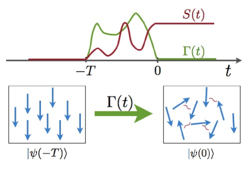
Figure 1: (Color online) Entanglement Storage Units protocol: a system is initially in a reference state $|\psi(-T)\rangle$, e.g. the ground state, and is optimally driven via a control field $\Gamma(t)$ in an entangled eigenstate $|\psi(0)\rangle$, protected from decoherence by an energy gap. $S(t)$ represents a generic measure of entanglement.

In this work we show that by means of a recently developed optimal control technique Doria_PRL11 ; Caneva_PRA11 it is possible to identify and prepare a many body quantum system in robust, long-lived entangled states (ESU states). More importantly, we drive the system towards ESU states without the need of any apriori information on the system, either about the eigenstates or about the energy spectrum. Indeed, we do not first solve the complete spectrum and eigenstates, which is an exponentially difficult problem in the system size. Recently, optimal control has been used to drive quantum systems in entangled states or to improve the generation of entanglement Platzer_PRL10 . However, here we have in mind a different scenario: to exploit the control to steer a system into a highly entangled state that is stable and robust even after switching off the control (see Fig. 1). Moreover we want to outline the fact that we do not choose the goal state, but only its properties. In the following we show that ESU states are gap-protected entangled eigenstates of the system Hamiltonian in the absence of the control, and that for an experimentally relevant model is indeed possible to identify and drive the system into the ESU states. We show that the ESU states, although not being characterized by the maximal entanglement sustainable by the system, are characterized by entanglement that grows with the system size. Once a good ESU state has been detected, due to its robustness it can be stored, characterized, and thus used for later quantum information processing.
Here we provide an important example of this approach, based on the the Lipkin-Meshkov-Glick (LMG) model Lipkin_NP65 , a system realizable in different experimental setups Baumann_NAT10 ; Buecker_NAT11 ; we prepare an ESU maximizing the Von Neumann entropy of a bipartition of the system and we model the action of the surrounding environment with noise terms in the Hamiltonian. However, our protocol is compatible with different entanglement measures and different models, like the concurrence between the extremal spins in an Ising chain, see Sec. V. Notice that with a straightforward generalization it can be adapted to a full description of open quantum systems inpreparation .

The article is organized as follows: in Sec. II the general protocol to steer a system onto ESU state is presented; in Sec. III we consider the application of the protocol to the Lipkin-Meshkov-Glick model; in Sec. IV we discuss the effect of a telegraphic classical noise onto the protocol; in Sec. V we test the protocol into an Ising spin chain, and finally in Sec. VI we present the conclusions of our work.

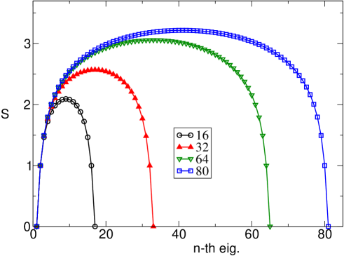
Figure 2: (Color online) LMG model: Static entanglement $S$ of the eigenstates at $\tilde{\Gamma}=10$ for different system sizes $N=16,32,64,80$. The eigenstates are ordered according to their energy, i.e. $n=1$ corresponds to the ground state.

II ESU protocol

As depicted in Fig. 1, we consider the general scenario of a system represented by a tunable Hamiltonian $H[\Gamma]$, where $\Gamma(t)$ is the control field, and initialized in a state $|\psi_{in}\rangle$ that can be easily prepared. We assume that the control field $\Gamma(t)$ can be modulated only in the finite time interval $[-T,0]$; outside of this interval, for $t<-T$ and $0<t$, we impose $\Gamma\equiv\tilde{\Gamma}$ (e.g. absence of control). According to our protocol, at the end of the control procedure, i.e. once the control field is brought back to the value $\tilde{\Gamma}$, the system has been prepared in a state with desired properties (for instance high entanglement), stable in absence of the control and robust against noise and perturbations.
Optimal control has been already used to enhance a given desired property without targeting an apriori known state; unfortunately the results of such optimization are usually fragile and ideally require a continuous application of the control in order to be stabilized Platzer_PRL10 . However in practical situations a continuous application of control can be unrealistic, being either simply impossible or too expensive in terms of resources. An example is the initialization of a quantum register that has to be physically moved into different spatial locations (like a portable memory support), or if the control field used to initialize has to be switched on and off in order to manipulate different parts of the apparatus; in such situations indeed the register should be stable also once disconnected from the device employed for its initialization. Consequently in certain applications, a procedure capable to prepare quantum targets intrinsically stable even in the absence of sustained external manipulations is not only highly desirable but also crucial. The main contribution of our work is exactly to move a step forward in this direction, proposing a flexible recipe to improve the stability of the outcome of a generic optimization process.
The simply idea behind our method is the following: as it is well known, in a closed system, the evolution of an arbitrary state is driven by Schrödinger equation $i\hbar|\dot{\psi}(t)\rangle=H(t)|\psi(t)\rangle$. Assuming that, as in the absence of control, the Hamiltonian is constant $H(t)=H[\tilde{\Gamma}]$, we can evaluate the extent of the deviation induced by the time evolution in an infinitesimal time $dt$ after switching off the control Anandan_PRL90 :

$$1-|\langle\psi(t)|\psi(t+dt)\rangle|^{2}=\Delta\tilde{E}^{2}dt^{2}/\hbar^{2}+O(dt^{3}),$$ (1)

where $\Delta\tilde{E}=\sqrt{\langle\psi(t)|H^{2}[\tilde{\Gamma}]|\psi(t)\rangle-\tilde{E}^{2}}$ and $\tilde{E}=\langle\psi(t)|H[\tilde{\Gamma}]|\psi(t)\rangle$ correspond respectively to the energy fluctuations and the energy of the Hamiltonian in absence of control. Then from Eq. (1) it is clear that an arbitrary state is stabilized by minimizing the quantity $\Delta\tilde{E}$. In particular, by reaching the condition $\Delta\tilde{E}=0$, the system is also prepared in an eigenstate of $H[\tilde{\Gamma}]$.
Our protocol relies on the use of optimal control implemented through the Chopped RAndom Basis (CRAB) techniqueDoria_PRL11 ; Caneva_PRA11 . The CRAB method consists in expanding the control field onto a truncated basis (e.g. a truncated Fourier series) and in minimizing an appropriate cost function with respect to the weights of each component of the chopped basis (see Doria_PRL11 ; Caneva_PRA11 for details of the method).
In particular, for the ESU protocol a CRAB optimization is performed with the goal of minimizing the cost function $\mathcal{F}$:

$$\mathcal{F}(\lambda)_{|\psi(0)\rangle}=-S+\lambda\frac{\Delta\tilde{E}}{\tilde{E}},$$ (2)

where $S$ represents a measure of entanglement, $\lambda$ is a Lagrange multiplier, and the cost function is evaluated on the optimized evolved state $|\psi(0)\rangle$ produced with a control process active in the time interval $[-T,0]$. As discussed previously and shown in the following, the inclusion in $\mathcal{F}$ of the constraint on the energy fluctuations is the crucial ingredient to stabilize the result of the optimization also for times $t>0$, that is once the control has been switched off.
We conclude this section stressing a couple of important advantages of our protocol with respect to possible other approaches to the problem, like for instance evaluating all the eigenstates of the system and picking up among them the state(s) with the desired properties. First, in our protocol we never compute the whole spectrum of the system, but we simply require to evaluate the energy and the energy fluctuations into the evolved state, see Eq. (2); therefore our procedure can be applied also to situations in which it is not possible to compute all the eigenstates of the Hamiltonian (e.g. many-body non integrable systems or DMRG simulations or experiments including a feedback loop). Furthermore it can occur that none of the eigenstates of the system owns the desired property we would like to enhance; then by simply considering the eigenstates one could not gain any advantage. On the contrary, also in this situation, with our protocol it is possible to identify states that, even though different from exact eigenstates, anyway show an enhanced robustness, like the optimal state found in the considered scenario, see Sec. V.

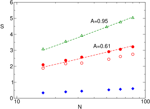
Figure 3: (Color online) LMG model: Ground state entanglement at the critical point of the (full blue diamonds); central eigenstate entanglement at $\tilde{\Gamma}=10$ (full red circles); maximal eigenstate entanglement obtained with the optimization for $\lambda\neq 0$ (empty red circles) and $\lambda=0$ (green triangle). The red (green) dashed line is numerical fit $A\cdot\log_{2}(N/2+1)$ with $A=0.61$ ($A=0.95$).

III ESU and Lipkin-Meshkov-Glick model

We decided to apply the protocol to the Lipkin-Meshkov-Glick modelLipkin_NP65 because it represents an interesting prototype of the challenge we address: it describes different experimental setups Baumann_NAT10 ; Buecker_NAT11 , and the entanglement properties of the eigenstates are in general not known. Indeed, the entanglement properties of the eigenstates of one-dimensional many-body quantum systems have been related with the corresponding conformal field theories Alba_JSTAT09 ; however for the LMG model, to our knowledge, this study has never been performed and a conformal theory is not available Latorre_JPA09 . Finally, the optimal control problem we address is highly non-trivial as the control field is global and space-independent with no single-site addressability Platzer_PRL10 .

The LMG Hamiltonian describes an ensemble of spins with infinite-range interaction and is written asBotet_PRB83 :

$$H=-\frac{C}{N}\sum^{N}_{i<j}\sigma_{i}^{x}\sigma_{j}^{x}-\Gamma(t)\sum_{i}^{N}\sigma_{i}^{z},$$ (3)

where $N$ is the total number of spins, $\sigma_{i}^{\alpha}$’s ($\alpha=x,y,z$ ) are the Pauli matrices on the $i$th site and $C$ is a constant measuring the intensity of the spin-spin interaction. By introducing the total spin operator $\vec{J}=\sum_{i}\vec{\sigma}_{i}/2$, the Hamiltonian can be rewritten, apart from an additive constant and a constant factor as

$$H=-\frac{1}{N}J_{x}^{2}-\Gamma J_{z},$$ (4)

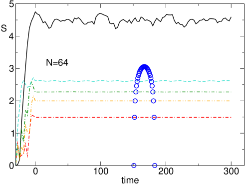
Figure 4: (Color online) Entanglement entropy $S(t)$ as a function of time (time unit $C^{-1}$) for different $\lambda$ values: $\lambda=0$ (black) continuous, $\lambda=5$ (red) dash-dash-dotted, $\lambda=1.8$ (green) dot-dashed, $\lambda=1.9$ (orange) dot-dot-dashed, $\lambda=1.2$ (cyan) dashed line. Blue circles represent the entropy of the eigenstates for $N=64$ and $\tilde{\Gamma}=10$.

(from now on we set $C=1$ and $\hbar=1$). The symmetries of the Hamiltonian imply that the dynamics is restricted to subspaces of fixed total magnetization $J$ and fixed parity of the projection $J_{z}$; a convenient basis for such subspaces is represented by the Dicke states $|J,J_{z}\rangle$ with $-J<J_{z}<J$ Latorre_PRA05 . In the thermodynamical limit the system undergoes a 2nd order QPT from a quantum paramagnet to a quantum ferromagnet at a critical value of the transverse field $|\Gamma_{c}|=1$. There is no restriction to the reference value $\tilde{\Gamma}$ and to the initial state $|\psi_{in}\rangle$: we choose $\tilde{\Gamma}\gg 1$, corresponding to the paramagnetic phase and as initial state $|\psi_{in}\rangle$, the ground state of $H[\tilde{\Gamma}]$, i.e. the separable state in which all the spins are polarized along the positive $z$-axis Baumann_NAT10 . A convenient measure of the entanglement in the LMG model is given by the von Neumann entropy $S_{L,N}=-{\rm Tr}(\rho_{L,N}\log_{2}\rho_{L,N})$ associated to the reduced density matrix $\rho_{L,N}$ of a block of $L$ spins out of the total number $N$, which gives a measure of the entanglement present between two partitions of a quantum system Latorre_PRA05 . In our analysis we consider two equal partitions, i.e. $S\equiv S_{N/2,N}$. Note that the maximally entangled state at a fixed size $N$ is given by $\rho_{M}={\bf 1}/(N/2+1)$ and $S_{\rho_{M}}=\log_{2}(N/2+1)$ Latorre_PRA05 . In Fig. 2 we report the entanglement $S_{N/2,N}$ of the eigenstates deeply inside the paramagnetic phase at $\tilde{\Gamma}=10$, for systems of different sizes. Clearly, also far from the critical point $\Gamma=1$ many eigenstates possess a remarkable amount of entanglement that scales with the system size. The effect is shown more clearly in Fig. 3, where the entanglement of the central eigenstate (red full circles) at $\tilde{\Gamma}=10$ is compared with the entanglement of the ground state at the critical point (full blue diamonds). Both sets of data show a logarithmic scaling with the size, but the entanglement of the central eigenstate is systematically higher and grows more rapidly.

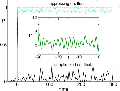
Figure 5: (Color online) Survival probability $P(t)$ as a function of time (time unit $C^{-1}$) for different $\lambda$ values: $\lambda=0$ (black) continuous, $\lambda=5$ (red) dash-dash-dotted, $\lambda=1.8$ (green) dot-dashed, $\lambda=1.9$ (orange) dot-dot-dashed, $\lambda=1.2$ (cyan) dashed line. Inset: Optimal driving field $\Gamma(t)$ for $\lambda=1.8$ and $N=64$.

Dynamics.— We initialize the system in the non-entangled ground state of the Hamiltonian $H[\tilde{\Gamma}]$ with $1\ll\tilde{\Gamma}=10$ so that in the absence of control, i.e. for $\Gamma\equiv\tilde{\Gamma}$ independent of time, the state $|\psi_{in}\rangle$ does not evolve apart from a phase factor. After the action of the CRAB-optimized driving field $\Gamma(t)$ for $t\in[-T,0]$ the state is prepared in $|\psi(0)\rangle$ (a typical optimal pulse is shown in the inset of Fig.  5), and we observe the evolution of the state over times $t>0$. The behavior of the entanglement is shown in Fig. 4 for different values of the weighing factor $\lambda$ and $N=64$. For $\lambda=0$ highly entangled states are produced, however the entanglement $S(t)$ oscillates indefinitely with the time. On the contrary, if the energy fluctuations are included in the cost function ($\lambda\neq 0$), the optimal driving field steers the system into entangled eigenstates of $H[\tilde{\Gamma}]$, as confirmed by the absence of the oscillations in the entanglement and by the entanglement eigenstate reference values (empty blue circles). These results are confirmed by the survival probability in the initial state $P(t)=|\langle\psi(0)|\psi(t)\rangle|^{2}$ reported in Fig. 5: the state prepared with $\lambda=0$ decays over very fast time scales $\tau_{0}$, while for $\lambda\neq 0$ it remains close to the unity for very long times $\tau_{\lambda}>>\tau_{0}$. The small residual oscillations for $N=64$ and $\lambda=1.2$ are due to the fact that in this case the optimization leads to a state corresponding to an eigenstate up to $98\%$. We repeated the optimal preparation for different system sizes and initial states, and show the entanglement of the optimized states for $\lambda=0$ (empty green triangles) and $\lambda\neq 0$ ( $\Delta\tilde{E}/\tilde{E}<0.05$, $P>95\%$ empty red circles) for different system sizes in Fig. 3. In all cases a logarithmic scaling with the size is achieved.

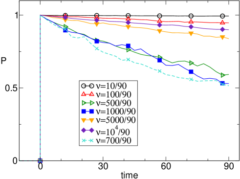
Figure 6: (Color online) Survival probability $P(t)$ as a function of time (time unit $C^{-1}$), averaged over $30$ noise instances for $I_{\alpha}=I_{\beta}=0.2$, $N=64$, $\lambda=1.8$, and different noise frequencies. The worst case (dashed line with crosses) is for $\nu_{R}=700/(90C^{-1})=7.8C$.

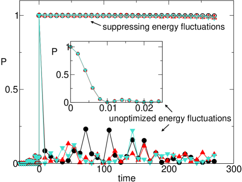
Figure 7: (Color online) Survival probability $P(t)$ as a function of time (time unit $C^{-1}$) for three realizations of the noise with $I_{\alpha}=I_{\beta}=0.01$ at frequency $\nu_{R}$, $N=64$, and $\lambda=1.8$ (empty symbols) or $\lambda=0$ (full symbols). Inset: Blow up of the region around $t=0$ for the $\lambda=0$ case.

IV Random telegraph noise

A reliable ESU should be robust against external noise and decoherence even when the control is switched off, in such a way that it could be used for subsequent quantum operations. In order to test the robustness of the optimized states, we model the effect of decoherence by adding a random telegraph noise and we monitor the time evolution in such noisy environment Nielsen_Chuang:book . In particular we study the evolution induced by the Hamiltonian

$$H=-\frac{1}{N}[1+I_{\alpha}\alpha(t)]J_{x}^{2}-\tilde{\Gamma}[1+I_{\beta}\beta(t)]J_{z}$$ (5)

where $\alpha(t),\beta(t)$ are random functions of the time with a flat distribution in $[-I_{j},I_{j}]$ ($j=\alpha,\beta$), changing random value every typical time $1/\nu$. The case $I_{\alpha}=I_{\beta}=0$ corresponds to a noiseless evolution. The first important observation is that the frequency $\nu$ of the signal fluctuations is crucial in determining its effects facchi05 . Indeed in Fig. 6, the survival probability $P(t)$ is plotted as a function of the time in the presence of a strong noise, $I_{\alpha}=I_{\beta}=0.2$, for a system of $N=64$ spins and for a given initial optimal state obtained with $\lambda=1.8$ (see Fig. 4). When $\nu$ is either too low (empty circles) or too high (full diamonds) the effect of the noise is reduced; however around a resonant frequency $\nu_{R}$ (dashed line with crosses) its effect is enhanced and the state is quickly destroyed. We checked that the resonant frequency is the same for different eigenvalues, different sizes, and different noise strengths (data not shown), reflecting the fact that in the paramagnetic phase ($\tilde{\Gamma}\gg 1$) the gap separating the eigenstates is proportional to $\tilde{\Gamma}$ independently of the size of the system and of the state itself, see Eq. (4). Therefore we analyze this worst case scenario, setting $\nu=\nu_{R}$ from now on. In Fig. 7

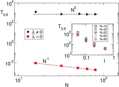
Figure 8: (Color online) Time $T_{0.8}$ required to reduce the survival probability $P$ below $0.8$ for different prepared states $|\psi(0)\rangle$ with $\lambda=0$ (red squares) and $\lambda\neq 0$ corresponding to the second eigenstate of the even parity sector of $J_{z}$ (black triangles) as a function of the system size $N$. The dashed lines are fits of the four rightmost points (biggest system sizes) resulting in $N^{-0.97}$ and $N^{-0.03}$ respectively. Inset: Time $T_{0.8}$ as a function of the intensity $I=I_{\alpha}=I_{\beta}$ of the disorder for different system sizes $N$.

we compare the survival probability $P(t)$ for three instances of the disorder at the resonant frequency with an intensity of the disorder $I_{\alpha}=I_{\beta}=0.01$. The noise-induce dynamics of the states obtained optimizing only with respect to the entanglement (i.e. setting $\lambda=0$, full symbols in Fig. 7) drastically depends on the (in general unknown) details of the noise affecting the system; thus, such states cannot be used as ESU. Viceversa the states prepared with $\lambda\neq 0$ (empty symbols in Fig. 7) turn out to be stable, noise-independent, and long-living entanglement. Finally, in Fig. 8 we study the decay times of the survival probability $P(t)$ studying the time $T_{0.8}$ needed to drop below a given threshold $P_{min}=0.8$ as a function of the system size $N$ and of the intensity of the disorder $I=I_{\alpha}=I_{\beta}$ (inset). These results clearly show that $T_{0.8}$ for ESU states is almost independent from the system size, reflecting the fact that the energy gaps in this region of the spectrum are mostly size independent. Notice that, on the contrary, $T_{0.8}$ for maximally entangled states decays linearly with the system size and that there are more than four orders of magnitude of difference in the decay times $\tau_{\lambda}$ and $\tau_{0}$. Finally, the inset of Fig. 8 shows that the scaling of $T_{0.8}$ with the noise strength for ESU states is approximately a power law and again depends very weakly on the system size $N$.

V Ising model: concurrence between extremal spins

In our previous discussion we focused our attention onto the optimization of the Von Neumann entropy of eigenstates other than the ground state of the LMG model, in order to show the effectiveness of our protocol in controlling the dynamics and unexplored properties of many-body systems.

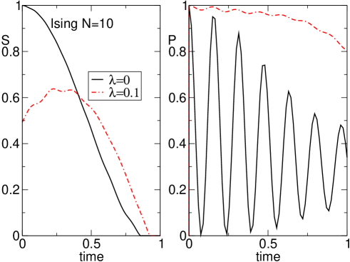
Figure 9: (Color online) Concurrence $S(t)$ between extremal spins (left panel) and survival probability $P(t)$ (right panel) as a function of time (time units $C^{-1}$) in an Ising chain with $N=10$ spins for two different $\lambda$ values: $\lambda=0$ black continuous line and $\lambda=0.1$ red dot-dashed line.

However aiming at demonstrating the generality of the method, in this section we would like to present briefly the application of our protocol to a different situation, closer to the typical problems encountered in quantum information: in particular we are showing how it is possible to stabilize the concurrence between the extremal spins of an open Ising chain.
The Hamiltonian of the ordered one-dimensional Ising model with nearest neighbor interaction is given by:

$$H=-C\sum^{N-1}_{i}\sigma_{i}^{x}\sigma_{i+1}^{x}-\Gamma(t)\sum_{i}^{N}\sigma_{i}^{z},$$ (6)

where the transverse field $\Gamma(t)$ is our control field. We assume that the system can be easily prepared in the ground state at a large value of the control field $\tilde{\Gamma}=10$, in which all the spins are polarized along the positive $z$-direction. The aim of the control is to enhance the concurrence between the first and the $N$-th spin of the chain, possibly stabilizing the state. The concurrence between two spins is defined as $S={\rm max}\{0,e_{1}-e_{2}-e_{3}-e_{4}\}$, where the $e_{i}$’s are the eigenvalues in decreasing order of the Hermitian matrix $R=\sqrt{\sqrt{\rho}\tilde{\rho}\sqrt{\rho}}$, $\rho$ is the reduced density matrix of the two extremal spins, and $\tilde{\rho}=(\sigma_{y}\otimes\sigma_{y})\rho^{*}(\sigma_{y}\otimes\sigma_{y})$ is the spin-flipped state Wootters_PRL98 .
At a large value of the transverse field, the eigenstates of the Hamiltonian are the classical states represented by all the possible up-down combinations of $N$ spins, and states with the same numbers of flipped spins, though in different positions, are degenerate. A naive approach to build stable entangled states would then require a search for possibly entangled states in each degenerate subspace at a given energy. Such a search however represents a highly non trivial task, due to the strong constraint imposed by requiring non vanishing concurrence: again a suitable recipe for such a search should be provided and is non-trivial to find. On the contrary our protocol proposes an answer to the task without requiring any diagonalization, while automatically performing the search, therefore offering a clear advantage.
We perform a CRAB optimization in the time interval $[-T,0]$ minimizing the function $\mathcal{F}(\lambda)_{|\psi(0)\rangle}=-S+\lambda\Delta\tilde{E}$, in which now $S$ is the concurrence; then at the time $t=0$ the control is switched off, the value of the field is kept constant ($\Gamma(t)=\tilde{\Gamma}$ for $t>0$), and we observe the evolution of the optimized state. In Fig. 9 we show the behavior of the concurrence $S(t)$ and of the survival probability $P(t)=\left({\rm Tr}\sqrt{\sqrt{\rho(t)}\rho(0)\sqrt{\rho(t)}}\right)^{2}$, excluding ($\lambda=0$ black continuous line) and including ($\lambda=0.1$ red dot-dashed line) the energy fluctuation term in the optimization procedure. As shown in the picture, although, as expected, the concurrence is smaller when $\lambda\neq 0$, the survival probability is stabilized by a factor bigger than $50$ in time with respect to the $\lambda=0$ case.

VI Conclusions

Exploiting optimal control we proposed a method to steer a system into apriori unknown eigenstates satisfying desired properties. We demonstrated, on a particular system, that this protocol can be effectively used to build long-lived entangled states with many-body systems, indicating a possible implementations of an Entanglement Storage Unit scalable with the system size. The presented method is compatible with different models (e.g. LMG and Ising) and measures of entanglement (e.g. von Neumann entropy and concurrence) and it can be extended to any other property one is interested in, as for example the squeezing of the target state inpreparation . It can be applied to different systems with apriori unknown properties: optimal control will select the states (if any) satisfying the desired property and robust to system perturbations. We stress that an adiabatic strategy is absolutely ineffective for this purpose, as transitions between different eigenstates are forbidden. Applying this protocol to the full open-dynamics description of the system, e.g. via a CRAB optimization of the Lindblad dynamics as done in caruso11 , will result in an optimal search of a Decoherence Free Subspace (DFS) with desired properties DFS . If no DFS exists, the optimization would lead the system in an eigenstate of the superoperator with longest lifetime and desired properties inpreparation . Although the state so prepared may be unstable over long times, it represents the best and most robust state attainable, and additional (weak) control might be used to preserve its stability. Finally, working with excited states would reduce finite temperature effects, relaxing low temperatures working-point conditions, simplifying the experimental requirements to build a reliable ESU.

We acknowledge discussions with M. D. Lukin, and support from the EU projects AQUTE, PICC, the SFB/TRR21 and the BWgrid for computational resources.

References

- (1) Nielsen M and Chuang I L 2000 Quantum Computation and Quantum Information (Cambridge University Press)
- (2) Baumann K, Guerlin C, Brennecke F and Esslinger T 2010 Nature 464 1301
- (3) Amico L, Fazio R, Osterloh A and Vedral V 2008 Rev. Mod. Phys. 80 517
- (4) Vidal G, Latorre J, Rico E and Kitaev A 2003 Phys. Rev. Lett. 90 227902
- (5) Alba V, Fagotti M and Calabrese P 2009 J. Stat. Mech. p. P10020
- (6) Alcaraz F C, Berganza M and Sierra G 2011 Phys. Rev. Lett. 106 201601
- (7) Doria P, Calarco T and Montangero S 2011 Phys. Rev. Lett. 106 190501
- (8) Caneva T, Calarco T and Montangero S 2011 Phys. Rev. A 84 022326
- (9) Platzer F, Mintert F and Buchleitner A 2010 Phys. Rev. Lett. 105 020501
- (10) Lipkin H J, Meshkov N and Glick A J 1965 Nucl. Phys. 62 188
- (11) Bücker R, Grond J, Manz S, Berrada T, Betz T, Koller C, Hohenester U, Schumm T, Perrin A and Schmiedmayer J 2011 Nat. Phys. 7 608
- (12) Caneva T et al in preparation
- (13) Anandan J and Aharonov Y 1990 Phys. Rev. Lett. 65 1697
- (14) Botet R and Jullien R 1983 Phys. Rev. 28 3955
- (15) Latorre J I and Riera A 2009 J. Phys. A: Math. Theor. 42 504002
-
(16)
Latorre J I, Orus R, Rico E and Vidal J 2005 Phys. Rev. A 71 064101
Barthel T, Dusuel S and Vidal J 2006 Phys. Rev. Lett. 97 220402
For the solution of the LMG model in the thermodynamical limit see also:
Ribeiro P, Vidal J and Mosseri R 2008 Phys. Rev. E 78 021106 - (17) Facchi P, Montangero S, Fazio R and Pascazio P 2005 Phys. Rev. A 71 060306
- (18) Wootters W K 1998 Phys. Rev. Lett. 80 2245
- (19) Caruso F, Montangero S, Calarco T, Huelga S F and Plenio M B 2011 Preprint arXiv:1103.0929
-
(20)
Palma G M, Suominen K A and Ekert A K 1996 Proc. Roy. Soc. Lond. A 452 567
Duan L M and Guo G C 1997 Phys. Rev. Lett. 79 1953
Zanardi P and Rasetti M 1997 Phys. Rev. Lett. 79 3306