Time-dependent density-functional and reduced density-matrix methods for few electrons: Exact versus adiabatic approximations

Abstract

To address the impact of electron correlations in the linear and non-linear response regimes of interacting many-electron systems exposed to time-dependent external fields, we study one-dimensional (1D) systems where the interacting problem is solved exactly by exploiting the mapping of the 1D $N$-electron problem onto an $N$-dimensional single electron problem. We analyze the performance of the recently derived 1D local density approximation as well as the exact-exchange orbital functional for those systems. We show that the interaction with an external resonant laser field shows Rabi oscillations which are detuned due to the lack of memory in adiabatic approximations. To investigate situations where static correlations play a role, we consider the time-evolution of the natural occupation numbers associated to the reduced one-body density matrix. Those studies shed light on the non-locality and time-dependence of the exchange and correlation functionals in time-dependent density and density-matrix functional theories.

1 Introduction

Since its invention in 1984 time-dependent density-functional theory (TDDFT) has become one of the major tools for describing time-dependent phenomena of electronic systems [1, 2]. Despite its success, several important questions remain open. A prominent example are double excitations [3], which cannot be described with adiabatic approximations to the exchange-correlation (xc) kernel [4]. Other examples include the description of memory [5], charge-transfer excitations [6], Rabi oscillations [7], and population control [8, 9]. Also, the construction of functionals for certain observables can be problematic, like e.g. double-ionization in strong laser fields where one strategy rests on expressing the pair-correlation function as a functional of the time-dependent density [10].

In many cases, there is little knowledge about how the dynamics of the many-body system interacting with an arbitrary external time-dependent field is mapped onto the non-interacting (time-dependent) Kohn-Sham system. Here, one-dimensional systems can provide insight since these systems can be exactly diagonalized and subsequently propagated in time for a small number of electrons. We provide insight into the limitations of adiabatic functionals, especially for describing non-linear electron dynamics exemplified by the case of Rabi oscillations.

This article is organized as follows, we first highlight the exact mapping of a many-electron system onto an $N$-dimensional one-electron problem and the selection of proper fermionic solutions. Then, we discuss the recently developed one-dimensional local density approximation (LDA) and its performance for calculating linear and non-linear response. We use the LDA as well as exact exchange (EXX) to investigate the description of double excitations and Rabi oscillations with adiabatic approximations. We then change from TDDFT to reduced density-matrix functional theory, where we discuss under which conditions adiabatic approximations provide a valid description. We conclude the paper with a short summary and perspectives.

Figure 1: Possible standard Young diagrams for the spatial part of the wave function for two [figures a) and b)] and three [figures c) to e)] electrons. There are maximally two columns in each diagram, one for each spin direction. Figures a) and b) correspond to the two electron singlet and triplet, respectively. For diagram c) the wave function is symmetrized for particles 1 and 2 and antisymmetrized for 1 and 3, while for diagram d) the symmetrization is with respect to particles 1 and 3 and the antisymmetrization with respect to 1 and 2. For diagram e) the wave function is antisymmetrized with respect to the interchange of any two particles.

2 One-dimensional model systems

The Hamiltonian for $N$ electrons moving in a general, possibly time dependent, external potential $v_{\rm ext}$ in one spatial dimension reads

$$H=\sum_{j=1}^{N}\left[-\frac{d^{2}}{2dx_{j}^{2}}+v_{\rm ext}(x_{j},t)\right]+\frac{1}{2}\sum_{\stackrel{{\scriptstyle\scriptstyle j,k=1}}{{j\neq k}}}^{N}v_{\rm int}(x_{j},x_{k}),$$ (1)

where $v_{\rm int}$ describes the electron-electron interaction (atomic units $e=m=\hbar=1$ are used throughout this paper). In one spatial dimension the singularity of the ordinary Coulomb interaction prevents electrons from passing the position of the singularity, both in the attractive and repulsive case. In order to avoid this unphysical behavior of the full Coulomb interaction we employ the so called soft-Coulomb interaction

$$v_{\rm soft-C}(x_{1},x_{2})=\frac{q_{1}q_{2}}{\sqrt{a^{2}+(x_{1}-x_{2})^{2}}}$$ (2)

instead [11]. Here, $q_{1}$ and $q_{2}$ describe the charges of the particles while $a$ is the usual softening parameter. We use $a=1$ for all our calculations. Mathematically, it is straightforward to show that the Hamiltonian (1) is equivalent to a Hamiltonian for a single particle in $N$ dimensions moving in an external potential

$$v_{\rm Ndim}(x_{1}...x_{N})=\sum_{j=1}^{N}v_{\rm ext}(x_{j})+\frac{1}{2}\sum_{\stackrel{{\scriptstyle\scriptstyle j,k=1}}{{j\neq k}}}^{N}v_{\rm int}(x_{j},x_{k})$$ (3)

consisting of all the contributions from $v_{\rm ext}$ and $v_{\rm int}$. The corresponding Schrödinger equation can, hence, be solved by any code which is able to treat non-interacting particles in the correct number of dimensions in an arbitrary external potential.

Due to the Hamiltonian being symmetric under particle interchange, $x_{j}\leftrightarrow x_{k}$, the solutions of the Schrödinger equation can be classified according to irreducible representations of the permutation group. For the simplest case of two interacting electrons both the symmetric and antisymmetric solutions are valid corresponding to the singlet and triplet spin configurations, respectively. For more than two electrons one needs to separately ensure that the spatial wave function is a solution to the $N$-electron problem. For example, a totally symmetric spatial wave function is a correct solution for a single particle in $N$ dimensions, however, for $N>2$ there is no corresponding spin function such that the total wave function has the required antisymmetry to be a solution of the $N$ particle problem in 1D. We solve this problem by symmetrizing the solutions according to all possible fermionic Young diagrams for the given particle number $N$ [12]. Fig. 1 shows all possible standard Young diagrams for the spatial part of the wave function for two and three electrons. As the spin of the electron is $1/2$, the Young diagrams for the spin part can maximally have two rows, one for each spin direction. The Young diagrams for the spatial part of the wave function are then given as the transpose of the respective spin diagram and, hence, have at most two columns. For two electrons there exist two diagrams corresponding to the singlet (Fig. 1 a) and triplet (Fig. 1 b) configurations. For three electrons, there exist two diagrams with two electrons in one spin channel and the remaining electron in the other channel (Fig. 1 c and d) and one diagram with all electrons having the same spin (Fig. 1 e).

In practice, we solve the Schrödinger equation in $N$ dimensions and then symmetrize each solution according to the Young diagrams for the given particle number. If none of the Young diagrams yields a non-vanishing solution after symmetrization the state does not describe a solution for spin-$1/2$ particles and is discarded. If a state yields a non-vanishing contribution for a given diagram the appropriately symmetrized state is normalized and used in further calculations.

The solution of higher dimensional problems within these symmetry restrictions has been implemented in the octopus computer program [13, 14]. The lowest energy solution is found to be purely symmetric and is, therefore, for $N>2$, discarded. With increasing number of electrons we also observe an increasing number of states which do not satisfy the fermionic symmetry requirements.

3 Local density approximation

The local density approximation for electrons interacting in one spatial dimension is derived from quantum Monte-Carlo calculations for a 1D homogeneous electron gas where the electrons interact via the soft-Coulomb interaction in Eq. (2)[15]. The correlation energy is parametrized in terms of $r_{s}$ and the spin polarization $\zeta=(N_{\uparrow}-N_{\downarrow})/N$ in the form

$$\epsilon_{c}(r_{s},\zeta) = \epsilon_{c}(r_{s},\zeta=0)$$

$$+\zeta^{2}\left[\epsilon_{c}(r_{s},\zeta=1)-\epsilon_{c}(r_{s},\zeta=0)\right]$$

with

$$\epsilon_{c}(r_{s},\zeta=0,1) = \!-\frac{1}{2}\frac{r_{s}+Er_{s}^{2}}{A+Br_{s}+Cr_{s}^{2}+Dr_{s}^{3}}$$ (5)

$$\times\ln(1+\alpha r_{s}+\beta r_{s}^{m})$$

which proves to be very accurate in the parameterization for 1D systems for different long-range interactions [16, 17, 15]. Note, that the above energy is given in Hartree units. To obtain a priori the exact high-density result known from the random-phase approximation, i.e.

$$\epsilon_{c}(r_{s}\rightarrow 0,\zeta=0) = -\frac{4}{\pi^{4}a^{2}}~{}r_{s}^{2},$$ (6)

$$\epsilon_{c}(r_{s}\rightarrow 0,\zeta=1) = -\frac{1}{2\pi^{4}a^{2}}~{}r_{s}^{2},$$ (7)

to leading order in $r_{s}$, we fix the ratio $\alpha/A$ to be equal to $8/(\pi^{4}a^{2})$ and $1/(\pi^{4}a^{2})$ for $\zeta=0$ and $\zeta=1$, respectively. In both cases $m$ is limited to values larger than 1. As a result, the number of independent parameters in Eq. (5) is reduced to 7. In addition, for $a=1$ the denominator can be simplified by setting $B=0$. However, for smaller values of the softening parameter the linear term in the denominator is important for achieving agreement with the quantum Monte-Carlo results. The optimal values of the parameters are given in Tab. 1. For more details on the 1D QMC methodology and the parameterization procedure we refer to Refs. [16, 17].

	$\zeta=0$	$\zeta=1$
A	18.40(29)	5.24(79)
B	0.0	0.0
C	7.501(39)	1.568(230)
D	0.10185(5)	0.1286(150)
E	0.012827(10)	0.00320(74)
$\alpha$	1.511(24)	0.0538(82)
$\beta$	0.258(6)	$1.56(1.31)\cdot 10^{-5}$
m	4.424(25)	2.958(99)
$\Delta$	$6.7\cdot 10^{-5}$	$3.3\cdot 10^{-5}$

Table 1: Parameterization of the correlation energy of the 1D homogeneous electron gas for a softening parameter of $a=1$, spin unpolarized ($\zeta=0$) and fully polarized ($\zeta=1$) cases are given. The error in the last digits is given in parenthesis, while the average error, $\Delta$, (in Hartree) in the full density range is given in the last row.

We have implemented the 1D LDA for $a=1$ in both unpolarized and polarized versions in the octopus program [13, 14].

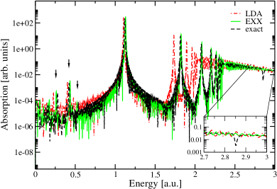
Figure 2: Linear (top) and non-linear (bottom) spectra of Be²⁺, calculated from the Fourier transformation of the dipole moment using a polynomial damping function, comparing the exact and the 1D LDA calculation. The inset in the bottom figure shows a zoom into the region from $2.7$ to $3.0$ Ha.

Fig. 2 shows the linear and non-linear absorption spectra of a 1D Be²⁺ system, i.e. with an external potential of

$$v_{\rm ext}^{\mathrm{Be}}(x)=\frac{-4}{\sqrt{x^{2}+a^{2}}}$$ (8)

containing two electrons. We use the LDA as an adiabatic approximation to the exact time-dependent exchange-correlation potential. The spectrum is calculated in linear response to a spatially constant perturbation at $t=0$, i.e. we apply an additional external electric field ${\cal E}$ in dipole approximation

$$v_{\rm ext}^{\mathrm{kick}}(x,t)=x{\cal E}_{0}\delta(t)$$ (9)

which gives an initial momentum to the electrons. The time propagations were performed in a box ranging from -150 to 150 bohr with absorbing boundary conditions [13] and a grid spacing of 0.2 bohr for a total propagation time of $10^{3}$ a.u. In the linear regime a kick of ${\cal E}_{0}=10^{-4}$ Ha/bohr was employed which was then increased to $0.01$ Ha/bohr to obtain the non-linear response. The values of the excitation energies can be found in Tab. 2. In linear response, we see five peaks in the LDA spectrum which compare well with the first five excitations in the exact case. As expected, the agreement is better for lower lying excitations and gets worse the closer we get to the continuum. As a guide for the eye we included the KS HOMO energy of the LDA calculation, $\epsilon_{\mathrm{HOMO}}=2.06$ Ha and the exact ionization potential of 2.41 Ha. The onset of the continuum itself appears at too low energies in the LDA calculation missing two more clearly visible peaks in the exact spectrum. In other words, the LDA fails to reproduce the proper Rydberg series, a behavior well known from 3D calculations. For comparison we also included the results from an EXX calculation (which for two electrons is adiabatic and equal to Hartree-Fock) which shows a slightly better agreement than LDA for the first three excitations but, more importantly, reproduces the Rydberg series due to the correct asymptotic behavior of the corresponding exchange potential. The quality of the EXX results also implies that correlation is of secondary importance in the system for $a=1$. The non-linear spectrum shows the same excitations as the linear spectrum and three additional peaks for the exact and the EXX calculation and two additional peaks in the LDA spectrum. Their energies are also listed in Tab. 2. Due to the spatial symmetry of the system all even order responses are zero and the first non-vanishing higher-order response is of third order. The frequency $\Omega_{1}=0.28$ Ha corresponds to an excitation from the second to the third excited state, where the transition from the ground to the second excited state is dipole forbidden and, hence, can only be reached in a two-photon process. The other two frequencies, $\Omega_{2}=0.42$ Ha and $\Omega_{3}=0.54$ Ha, correspond to the transitions from first to second and second to fifth excited state, respectively. Again, both the EXX and the LDA calculations yield a good description of the low lying excitations, only the third peak cannot be resolved in the LDA spectrum.

	$\omega_{1}$	$\omega_{2}$	$\omega_{3}$	$\omega_{4}$	$\omega_{5}$	$\omega_{6}$	$\omega_{7}$	$\Omega_{1}$	$\Omega_{2}$	$\Omega_{3}$
LDA	1.10	1.74	1.90	1.96	2.00	-	-	0.22	0.40	-
EXX	1.13	1.82	2.08	2.20	2.27	2.30	2.32	0.26	0.43	0.52
exact	1.12	1.81	2.08	2.19	2.26	2.29	2.32	0.28	0.42	0.54

Table 2: Excitation energies from linear and non-linear response of the 1D Be²⁺ atom corresponding to the spectra in Fig. 2. Excitations from linear response are denoted as $\omega$ while those from the non-linear spectrum are denoted with $\Omega$. All numbers are given in Hartree.

One feature of the exact spectrum that is missing from both the LDA and the EXX spectra is the small dip at 2.8 Ha, see inset in Fig. 2. It results from a Fano resonance [18, 19], i.e. the decay of an excited state into continuum states. It is missing from both approximate spectra due to the double-excitation character of the involved excited state. Double excitations in the linear regime can only be described in TDDFT if a frequency-dependent xc kernel is employed [4]. Any adiabatic approximation, however, leads to a frequency independent kernel. Hence, double excitations, as well as any resulting features, are missing from both the ALDA and the AEXX linear response spectra. Apart from the well-known shortcomings of not including double-excitations and not giving the correct Rydberg series, the 1D ALDA reproduces both the linear and the non-linear exact spectra quite well.

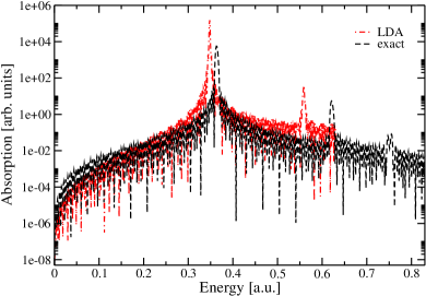
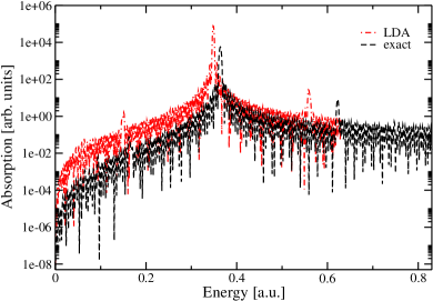
Figure 3: Discrete part of the linear (top) and non-linear (bottom) spectra of Be⁺, calculated from the Fourier transformation of the dipole moment using an exponential damping function, comparing the exact and the 1D LDA calculation. The exact ionization potential is at 0.83 Ha and the LDA HOMO at 0.63 Ha.

Fig. 3 shows the discrete part of the linear and non-linear spectra for the Be⁺ system, i.e. the external potential is given by Eq. (8) and the system contains three electrons. The ionization potential for the exact calculation is 0.83 Ha which is again underestimated by the LDA HOMO energy of 0.62 Ha. For this system the projection onto the Young diagrams becomes important with the lowest energy spatial solution being symmetric under exchange of any two variables. Therefore, it is not a valid solution for three fermions and, hence, discarded. The second lowest energy is doubly degenerate with the eigenstates corresponding to diagrams 1c and 1d. One of these states is then propagated with a kick strength of ${\cal E}_{0}=10^{-4}$ for the linear spectra and ${\cal E}_{0}=0.1$ for the non-linear spectra. The exact linear spectrum shows two transitions at 0.36 Ha and 0.62 Ha. Again, we observe that LDA underestimates these excitation energies giving 0.34 Ha and 0.55 Ha, respectively. The non-linear spectrum contains two more peaks in the exact spectrum at 0.09 Ha and 0.16 Ha which are, however, difficult to resolve. In the LDA spectrum only the peak at 0.16 Ha can be resolved. From the exact calculation of excited states we know that there should be several more transitions at very small frequencies which are accessible in non-linear response. Those are, however, very close to each other and, hence, more difficult to resolve. Attempts to improve the spectra in the small frequency region are currently in progress.

4 Double excitations

Figure 4: External $\cosh$-potential and single particle eigenvalues. In the non-interacting two-particle ground state both electrons occupy the lowest energy level in a singlet configuration.

In order to investigate double excitations in the linear-response spectrum we employ the following external potential

$$v_{\rm ext}^{\mathrm{cosh}}(x)=-\frac{v_{0}}{\cosh^{2}(kx)},$$ (10)

for which the one-particle problem can be solved analytically [12] and the resulting eigenvalues are given as

$$\epsilon_{j}=-\frac{k^{2}}{8}\left(\sqrt{1+\frac{8v_{0}}{k^{2}}}-1-2j\right)^{2}$$ (11)

for $j=0,1...$. Here, the term in parenthesis needs to be positive which restricts the number of bound states of the system. In other words, by choosing the two parameters $v_{0}$ and $k$ appropriately, one can create systems with any number of bound states. For our calculations we choose $k=1$ and $v_{0}=10$ which leads to the four bound single-electron states shown in Fig. 4.

	Symmetric well		Asymmetric well
State $j$	non-interact.	interacting	non-interact.	interacting	Spin
0	-16.00	-15.10	-16.92	-16.02	singlet
1	-12.50	-11.75	-13.21	-12.45	singlet
2	-12.50	-11.62	-13.21	-12.32	triplet
3	-10.00	-9.31	-10.52	-9.83	singlet
4	-10.00	-9.30	-10.52	-9.81	triplet
5	-9.00	-8.22	-9.48	-8.70	singlet
6	-8.50	-7.98	-8.90	-8.38	singlet
7	-8.50	-7.97	-8.90	-8.38	triplet
8	-8.00	-7.90	-8.45	-8.36	singlet
9	-8.00	-7.90	-8.45	-8.36	triplet

Table 3: Energies (in Hartree) for two-particle states in the symmetric well potential (10) and the asymmetric well Eq. (12) without interaction and with soft-Coulomb interaction, Eq. (2). The 5th excited state corresponds to a double excitation.

	Symmetric well			Asymmetric well
Excitation	Symmetry	non-interact.	interact.	non-interact.	interact.
$\Omega_{01}$	odd	-3.50	-3.48	-3.71	-3.70
$\Omega_{02}$	even	-6.00	-5.80	-6.40	-6.21
$\Omega_{11}$	even	-7.00	-6.88	-7.44	-7.32
$\Omega_{03}$	odd	-7.50	-7.13	-8.02	-7.64
$\Omega_{12}$	odd	-9.50	$\sim$ -9.28	-10.11	$\sim$ -9.91

Table 4: Excitation energies (in Hartree) for two particles in the symmetric well potential (10) and the asymmetric well Eq. (12) without interaction and with soft-Coulomb interaction, Eq. (2). $\Omega_{11}$ and $\Omega_{12}$ are double excitations. We also state the symmetry of the two-particle excited state for the symmetric well.

Putting two electrons into our system we calculate the total energies for non-interacting electrons as well as for electrons interacting via the soft-Coulomb interaction (2). The results for the first ten states are given in Tab. 3. As the energy differences between the interacting and non-interacting cases are small we can treat the many-body states as perturbed independent-particle states. This treatment is convenient because in the independent-particle picture double excitations are well defined: they describe transitions in which two electrons get excited with the excitation energies given as the sum of two single-particle excitations. The excitation energies for the different transitions are shown in Tab. 4. We note that the two-particle eigenstates of the symmetric well (10) can be chosen as eigenstates of the parity operator and, hence, can be classified as even and odd. For odd operators like the dipole operator the transitions from the ground state (even) to even two-particle excited states have zero oscillator strength. Nevertheless, these transitions can be visible beyond linear response. In addition, starting from the non-interacting ground state, doubly excited states have zero weight in the density response function because the density operator is a single particle operator. Thus, also the odd doubly excited two-particle states have zero oscillator strength for non-interacting particles. The 5th excited state of the non-interacting electrons can clearly be identified as a double excitation. This transition corresponds to both electrons getting promoted to the first excited state $\varepsilon_{1}$. As the energy differences between the interacting and non-interacting cases are small the 5th excited state of the interacting system is of double-excitation character as well. Unfortunately, however, this two-particle excited state is even under parity and, hence, the transition is dipole forbidden. The first double excitation which is dipole allowed is $\Omega_{12}$ which, in the independent-particle picture, corresponds to one electron getting promoted to the first excited state $\varepsilon_{1}$ and the other to the second excited state $\varepsilon_{2}$. It has an excitation energy of $9.50$ Ha in the non-interacting system. The first ionization potential of the system, however, is $8.00$ Ha which implies that the dipole allowed double excitation lies in the continuum part of the spectrum. In addition, $\Omega_{12}$ has zero weight in linear response for the non-interacting system because the transition matrix element vanishes as the final state differs from the initial state in two orbital occupations. For the interacting system, however, the two-particle spatial singlet wave function is no longer given as a product of the lowest energy single-particle orbital. A configuration interaction (CI) expansion of this wave function also contains terms which correspond to single excitations of the non-interacting particles. As a result, the double excitation $\Omega_{12}$ becomes accessible in linear response. This can be seen in Fig. 5, where we plot the absorption spectrum of the two-electron system both for interacting and non-interacting electrons. The spectrum was calculated in linear response to a spatially constant perturbation at $t=0$, see Eq. (9). We observe that the interacting spectrum shows a small dip at $\approx 9.4$ Ha which is close to the energy difference between the ground state and the dipole-allowed double excitation described earlier (as this excitation lies within the continuum its energy cannot be computed directly but an estimate can be found from $\Omega_{01}+\Omega_{02}$). We can clearly see that the transition lies within the continuum, or due to the calculation being done in a finite box, within the excitations to box states. Due to the nearby excitations to the continuum the frequency $\Omega_{12}$ of the bound transition is shifted slightly [18]. This excitations appears as a dip rather than a peak in the spectrum due to the absorbing boundary conditions which were employed in the calculation [19].

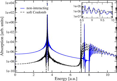
Figure 5: Linear response spectrum for two electrons in a $\cosh$ potential calculated from the Fourier transformation of the dipole moment using a polynomial damping function. For interacting electrons we observe an additional transition at $\approx 9.4$ Ha that corresponds to $\Omega_{12}$ (see inset).

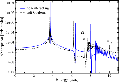
Figure 6: Linear response spectrum for two electrons in the modified $\cosh$ potential, Eq. (12), calculated from the Fourier transformation of the dipole moment using a polynomial damping function. Notice that for interacting electrons the double excitation $\Omega_{11}$ appears at $\approx 7.3$ Ha and $\Omega_{12}$ shifts to $\approx 10.0$ Ha.

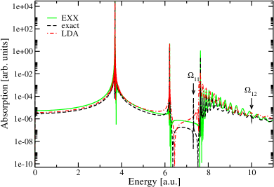
Figure 7: Linear response spectrum for two electrons in the modified $\cosh$ potential, Eq. (12), calculated from the Fourier transformation of the dipole moment using a polynomial damping function. For the DFT (EXX and LDA) spectra both double excitations $\Omega_{11}$ and $\Omega_{12}$ are missing.

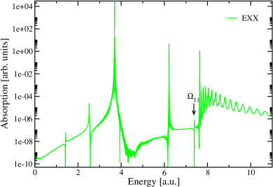
Figure 8: Non-linear response spectrum for two electrons using EXX in the modified $\cosh$ potential, Eq. (12), calculated from the Fourier transformation of the dipole moment using a polynomial damping function. The double excitation $\Omega_{11}$ appears at $\approx 7.4$ Ha (see arrow).

In order to investigate the double excitations which are dipole forbidden by symmetry, we break the spatial symmetry of the system by modifying the external potential to

$$v_{\rm ext}^{\mathrm{mod}}(x)=-\frac{v_{0}(1+0.5x)}{\cosh^{2}(kx)}.$$ (12)

As the Hamiltonian for this case no longer commutes with the parity operator, the eigenstates do not have a specific symmetry any longer. Therefore, the previously dipole forbidden transitions now have a finite oscillator strength. Also, the modification is small enough to leave the ordering of the states intact, i.e. the fifth excited state still has double-excitation character and the energies are approximately those of the symmetric system (see Tab. 3 for details). As we can see in Fig. 6 this leads to an additional peak slightly above 7.3 Ha which corresponds to the transition $\Omega_{11}$ from the ground state to the fifth excited state. In Fig. 7 we also include DFT linear response spectra for the symmetry-broken potential Eq. (12) using EXX and the 1D LDA functional of section 3 which are used as adiabatic approximations to the time-dependent xc potential. It is, therefore, not surprising that the double excitation $\Omega_{11}$ is missing from the resulting spectra [4, 20]. However, as we can see in Fig. 8, beyond linear response the double excitation $\Omega_{11}$ becomes visible even for the EXX functional, which is adiabatic, in the symmetry-broken potential.

5 Rabi oscillations

Rabi oscillations can occur when a system is exposed to an external laser field with frequency $\omega$, which is in resonance to a transition in the system. The system oscillates between two states with frequency $\Omega_{0}$ provided it can approximately be described as a two-level system. This is the case if the frequency $\omega$ is resonant to one specific transition in the system and the frequency of the oscillation between the states is much smaller than the frequency of the applied laser field. As will be discussed later, a small detuning of the applied laser from the exact resonant frequency still leads to Rabi oscillations, however, with increased frequency and smaller amplitude.

We analyze Rabi oscillations for a 1D two-electron model (see section 2) but note that the analysis can easily be extended to three dimensions and, using the single-pole approximation also to any number of electrons [21]. For ease of comparison we choose the same model as in [7] with the external potential

$$v_{\rm ext}^{\mathrm{Rabi}}(x,t)=-\frac{2}{\sqrt{x^{2}+1}}+x{\cal E}_{0}\sin(\omega t).$$ (13)

Eq. (13) describes a 1D Helium atom interacting with a monochromatic laser field of frequency $\omega$. We denote the eigenstates and eigenvalues of the Hamiltonian (1) with the external potential (13) as $\psi_{k}$ and $\epsilon_{k}$, respectively. In order for Rabi’s solution to be valid, the system under study needs to be an effective two-level system reducing the solution space to $\psi_{0}$ (ground state) and $\psi_{1}$ (dipole allowed excited state) with eigenenergies $\epsilon_{0}$ and $\epsilon_{1}$. The system then has a resonance at $\Delta=\epsilon_{1}-\epsilon_{0}$. The two-level approximation is valid if the two conditions

$$\frac{\delta}{\Delta}<<1,\quad\Omega_{0}<<\omega$$ (14)

are satisfied, where $\delta=\omega-\Delta$ describes the detuning from the resonance and $\Omega_{0}=d_{10}{\cal E}_{0}$ is the Rabi frequency for a resonant laser, with $d_{10}=\langle\psi_{0}|\sum_{j}\hat{x}_{j}|\psi_{1}\rangle$ the dipole matrix element. In order to satisfy the second condition we choose ${\cal E}_{0}=0.0125\omega$ in Eq. (13). For the eigenvalues we obtain $\epsilon_{0}=-2.238$ Ha and $\epsilon_{1}=-1.705$ Ha which implies a resonant frequency of $\Delta=\epsilon_{1}-\epsilon_{0}=0.534$ Ha. The static dipole matrix element is $d_{10}=1.104$. The frequency $\omega$ of the applied field has been chosen to be close to the resonance, i.e. the detuning $\delta=\omega-\Delta$ is small.

For an effective two-level system the time-dependent two-electron wave function $\psi(x_{1},x_{2},t)$ can be written as a linear combination of ground and excited state, i.e.

$$\psi(x_{1},x_{2},t)=a_{0}(t)\psi_{0}(x_{1},x_{2})+a_{1}(t)\psi_{1}(x_{1},x_{2})$$ (15)

with $|a_{0}(t)|^{2}=n_{0}(t)$ and $|a_{1}(t)|^{2}=n_{1}(t)$ being the time-dependent level populations of the ground and excited states. Normalization of the wave functions then implies $n_{0}(t)+n_{1}(t)=1$. As the amplitude ${\cal E}_{0}$ and the frequency $\omega$ of the applied field ${\cal E}(t)$ are chosen such that the conditions (14) are fulfilled the Hamiltonian (1) can be projected onto a $2\times 2$ space. The time-dependent Schrödinger equation $i\partial_{t}|\psi(t)\rangle=\hat{H}|\psi(t)\rangle$ then reduces to a $2\times 2$ matrix equation of the form

$$i\partial_{t}\left({\begin{array}[]{c}a_{0}(t)\\ a_{1}(t)\\ \end{array}}\right)=\left({\begin{array}[]{cc}\epsilon_{0}&d_{10}{\cal E}(t)\\ d_{10}{\cal E}(t)&\epsilon_{1}\\ \end{array}}\right)\left({\begin{array}[]{c}a_{0}(t)\\ a_{1}(t)\end{array}}\right)$$ (16)

from which one can derive coupled differential equations for the level population $n_{1}(t)$ and the dipole moment $d(t)=\langle\psi(t)|\hat{x}_{1}+\hat{x}_{2}|\psi(t)\rangle=2d_{10}Re\left(a_{0}^{*}(t)a_{1}(t)\right)$. For the dipole moment we obtain

$$d(t)=2d_{10}\sqrt{n_{0}(t)n_{1}(t)}\cos(\omega t+\theta(t)),$$ (17)

where the Rabi frequency is included in the time dependence of the amplitude of the dipole moment through the time dependence of $n_{0}(t)$ and $n_{1}(t)$, and $\theta(t)$ is the phase difference of $a_{0}(t)$ and $a_{1}(t)$. Fulfillment of conditions (14) allows for the use of the rotating wave approximation (RWA) [22] which yields the following differential equation for $n_{1}(t)$

$$\partial^{2}_{t}n_{1}(t)=-\left(\delta^{2}+\Omega_{0}^{2}\right)n_{1}(t)+\frac{1}{2}\Omega_{0}^{2}$$ (18)

with initial conditions $n_{1}(0)=0$ and $\dot{n}_{1}(0)=0$. Eq. (18) describes a harmonic oscillator with a restoring force which increases with increasing detuning $\delta$. As a result, the frequency of the Rabi oscillations increases with increased detuning, while the maximum population of the excited state decreases as $n_{1}^{\mathrm{max}}=\Omega_{0}^{2}/(\Omega_{0}^{2}+\delta^{2})$.

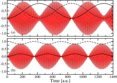
Figure 9: Dipole moment (red) and level populations $n_{1}(t)$ (solid black line) and $n_{0}(t)$ (dashed black line) from analytic solution of (16) using ${\cal E}_{0}=0.0125\omega$ for detuning $\delta=0.08\>\Omega_{0}$ ($0.0006$ Ha) (a) and $\delta=2.2\>\Omega_{0}$ ($0.016$ Ha) (b).

In Fig. 9 the time-dependent dipole moment $d(t)$ and the level populations $n_{0}(t)$ and $n_{1}(t)$ for $\delta=0.08\>\Omega_{0}$ and $\delta=2.2\>\Omega_{0}$ are shown. The effect of the detuning manifests itself in an incomplete population of the excited state and a consequent decrease in the amplitude of the envelope of the dipole moment that is proportional to $\sqrt{n_{0}n_{1}}$. For small detuning the minima and the maxima of $n_{1}$ coincide with minima of the envelope, but for larger detuning the dipole moment only goes to zero for the minima of $n_{1}$. In Fig.
reffig:dipolen1Lina the detuning is small but non-zero, hence, the neck at the minima of $n_{0}$. The neck grows with increasing $\delta$ and evolves into a maximum for Fig. 9b. Thus, the first minimum in Fig. 9b corresponds to one complete cycle and can be identified with the second minimum in Fig. 9a. We note that looking only at the dipole moment is insufficient to discern between resonant and detuned Rabi oscillations, only studying the level populations gives the complete picture.

For the system specified above a comparison between the analytic solution of Eqs. (17), (18) and the results of the time-propagation with the octopus code [13, 14] shows a perfect agreement, which confirms that the conditions (14) are fulfilled for the chosen values of ${\cal E}_{0}$ and $\omega$.

The KS Hamiltonian corresponding to (13) is given as

$$H_{s}=H_{s}^{0}+\sum_{j=1}^{N}\left(v_{\rm hxc}^{\rm dyn}(x_{j},t)+x_{j}{\cal E}_{0}\sin(\omega t)\right),$$ (19)

where the static KS Hamiltonian reads

$$H_{s}^{0}=\sum_{j=1}^{N}-\frac{\nabla_{j}^{2}}{2}+v_{\rm ext}(x_{j})+v_{\rm hxc}[\rho_{0}](x_{j}).$$ (20)

We denote the eigenfunctions of $H_{s}^{0}$ with $\phi_{k}(x)$ and their eigenvalues as $\epsilon_{k}^{s}$. As we are using a two-electron system, a single orbital is doubly occupied in the KS system. The time evolution of this orbital follows from the KS equation

$$i\partial_{t}\phi(x,t)=H_{s}\phi(x,t)$$ (21)

with the initial condition $\phi(x,t=0)=\phi_{0}(x)$. This equation is non-linear due to the dependence of the Hartree-exchange-correlation potential $v_{\rm hxc}$ on the density, $\rho(x,t)=2|\phi(x,t)|^{2}$. The time-dependent dipole moment $d(t)$ is an explicit functional of the density, i.e. $d(t)=\int x\rho(x,t)\,dx$. The exact KS system reproduces the exact many-body density $\rho(x,t)$ and, hence, the exact dipole moment $d(t)$. However, this need not be true for an approximate functional. Especially, using adiabatic approximations has been shown to have a dramatic effect on the calculated density during Rabi oscillations [7].

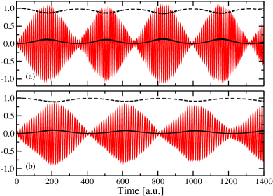
Figure 10: Dipole moment (red) and level populations $n_{1}^{s}$ (solid black line) and $n_{0}^{s}$ (dashed black line) for EXX (a) and ALDA (b).

Propagating with the EXX and ALDA (see section 3) results in the dipole moments shown in Fig. 10. The resonant frequencies are calculated from linear response which yields $\omega^{ALDA}=0.476$ Ha and $\omega^{EXX}=0.549$ Ha. We then apply a laser field in analogy to the exact calculation with an amplitude of ${\cal E}_{0}=0.0125\omega$ using the resonant frequency for each case. We observe in the level populations that both EXX and ALDA show the characteristic signatures of detuned Rabi oscillations despite the fact that the applied laser is in resonance with the system.

To clarify whether Rabi oscillations are well described in the context of adiabatic TDDFT we study the Hamiltonian (19) in more detail. The Hartree and xc potentials, $v_{\rm hxc}[\rho]$, render the KS differential equation non-linear. More specifically, for an adiabatic approximation the potential at time $t$ is a functional of the density at this time, i.e. $v_{\rm hxc}(t)=v_{\rm hxc}[\rho(t)]$. In the following, we show that $v_{\rm hxc}(t)$ introduces a detuning that drives the system out of resonance. We again rely on the conditions (14), i.e. describe the KS system as an effective two-level system. Therefore, the time-dependent orbital $\phi(x,t)$ is given as a linear combination of the ground-state KS orbital $\phi_{0}$ and the first excited state orbital $\phi_{1}$

$$\phi(x,t)=a_{0}^{s}(t)\phi_{0}(x)+a_{1}^{s}(t)\phi_{1}(x).$$ (22)

Projecting the KS Hamiltonian (19) onto the two-level KS space (22) yields the $2\times 2$ matrix

$$\left({\begin{array}[]{cc}\epsilon_{0}^{s}+\epsilon_{0}^{xc}(t)&d_{10}^{s}{\cal E}(t)+{\cal F}_{xc}(t)\\ d_{10}^{s}{\cal E}(t)+{\cal F}_{xc}^{*}(t)&\epsilon_{1}^{s}+\epsilon_{1}^{xc}(t)\\ \end{array}}\right)$$ (23)

with $d_{10}^{s}=\langle\phi_{1}|\hat{x}|\phi_{0}\rangle$, $\epsilon_{j}^{xc}(t)=\langle\phi_{j}|\hat{v}_{hxc}^{\rm dyn}(t)|\phi_{j}\rangle$, and ${\cal F}_{xc}(t)=\langle\phi_{0}|\hat{v}_{hxc}^{\rm dyn}(t)|\phi_{1}\rangle$. This matrix enters Eq. (16) to determine the coefficients $a_{0}^{s}(t)$ and $a_{1}^{s}(t)$. Compared to Eq. (16) we notice that each entry contains an additional term depending on $v_{\rm hxc}^{\rm dyn}$, i.e. both the electric field and the KS eigenvalues are modified. In order to investigate the consequences of the additional terms we use the EXX functional for which relatively simple analytic expressions for the additional matrix elements can be derived.

For the two-electron case investigated here, the Hartree-exchange-correlation potential $v_{\rm hxc}^{EXX}(x,t)$ is equal to half the Hartree potential and, hence, given as

$$v_{\rm hxc}^{EXX}(x,t)=\frac{1}{2}\int\frac{\rho_{0}(x^{\prime})+\delta\rho(x^{\prime},t)}{\sqrt{(x-x^{\prime})^{2}+a^{2}}}dx^{\prime},$$ (24)

where we split the total density $\rho(x,t)$ into a time-independent contribution $\rho_{0}(x)=2|\phi_{0}(x)|^{2}$ and a rest $\delta\rho(x,t)$ which can be calculated from Eq. (22) as

$$\delta\rho(x,t) = 2|a_{1}^{s}|^{2}(|\phi_{1}(x)|^{2}-|\phi_{0}(x)|^{2})$$

$$+4d_{10}^{s}Re(a_{0}^{s}(t)*a_{1}^{s}(t))\phi_{1}(x)\phi_{0}(x).$$

The part of Eq. (24) containing $\rho_{0}$ determines $v_{\rm hxc}[\rho_{0}]$ while $\delta\rho$ results in the additional $v_{\rm hxc}^{\rm dyn}$. Since $\phi_{0}$ and $\phi_{1}$ usually have opposite spatial symmetry (if the Hamiltonian is symmetric) the first term in Eq. (5) is symmetric while the second is antisymmetric. This results in the first term only contributing to the diagonal elements of the matrix (23) while the second term only contributes to the off-diagonal elements. Defining the level populations in the KS system as $n_{j}^{s}(t)=|a_{j}^{s}(t)|^{2}$ allows us to rewrite the contributions to the diagonal terms as

$$\epsilon_{j}^{xc}(t)=\lambda_{j}n_{1}^{s}(t),$$ (26)

where, for the EXX approximation, the coefficient $\lambda_{j}$ reads

$$\lambda_{j}=\int\!\!\int\frac{(|\phi_{1}(x^{\prime})|^{2}-|\phi_{0}(x^{\prime})|^{2})|\phi_{j}(x)|^{2}}{\sqrt{(x-x^{\prime})^{2}+a^{2}}}dxdx^{\prime}.$$ (27)

For the off-diagonal contribution we recall that $d^{s}(t)=2d_{10}^{s}Re(a_{0}^{s}(t)^{*}a_{1}^{s}(t))$, as in the exact case, and rewrite the contribution of $v_{\rm hxc}^{\rm dyn}(t)$ to the off-diagonal terms as a coefficient $g$ multiplied by the time-dependent dipole moment

$${\cal F}_{xc}(t)=g\frac{d^{s}(t)}{d_{10}^{s}}.$$ (28)

For the two-electron system in the EXX approximation $g$ is given as

$$g=\int\!\!\int\frac{\phi_{1}(x^{\prime})\phi_{0}(x^{\prime})\phi_{0}(x)\phi_{1}(x)}{\sqrt{(x-x^{\prime})^{2}+a^{2}}}dxdx^{\prime}.$$ (29)

The coefficient $g$ also enters the calculation of the resonant frequencies in linear response. Within the single-pole approximation the resonant frequency is given as $\omega_{0}^{s}=\sqrt{\Delta_{s}(\Delta_{s}+2g)}$ which for the EXX functional yields $\omega^{EXX}=0.532$ Ha. The deviation from the frequency calculated from time propagation of the Hamiltonian (19) in octopus is of the order of $3\%$, coinciding with the deviation of our system from a true two-level system which we estimate from $\left(1-(n_{0}^{s}(t)+n_{1}^{s}(t))\right)$. Using, as in the exact case, the RWA we obtain to leading order in $\lambda/\omega_{0}$ and $g/\omega_{0}$ the following equation of motion for the level population $n_{1}(t)$

$$\partial^{2}_{t}n_{1}^{s}(t)=-\left(\frac{\gamma^{2}}{2}n_{1}^{s}(t)^{2}+\Omega_{s}^{2}\right)n_{1}^{s}(t)+\frac{1}{2}\Omega_{s}^{2}$$ (30)

with $\Omega_{s}=d_{10}^{s}{\cal E}_{0}$ and $\gamma=\lambda-2g$. Neglecting the higher order terms in $\lambda/\omega_{0}$ and $g/\omega_{0}$ introduces an error of about 10% in favor of keeping the equation simple while still containing the important physical effects. Unlike Eq. (18) which represents a harmonic oscillator, Eq. (30) corresponds to an anharmonic quartic oscillator and its solution is given in terms of Jacobi elliptic functions [23]. Equivalently, Eq. (30) can be integrated numerically. Even though the oscillator is no longer harmonic the detuning still results in an increase of the restoring force. In other words, the adiabatic approximation introduces a time-dependent detuning proportional to $\gamma n_{1}^{s}(t)$.

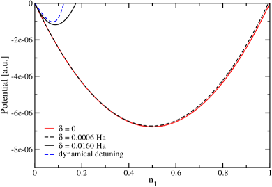
Figure 11: Potentials corresponding to the differential equations (18) and (30). The dynamical detuning leads to a quartic potential which has a similar effect to the potential as a large detuning.

Using the same 1D model system (13) as before and diagonalizing the Hamiltonian (19) gives for the bare KS eigenvalues $\epsilon_{0}^{EXX}=-0.750$ Ha and $\epsilon_{1}^{EXX}=-0.257$ Ha which yields $\Delta_{s}=0.494$ Ha. For the various matrix elements we obtain $d_{10}^{s}=0.897$, $g=0.071$, $\lambda=-0.125$, and $\gamma=-0.268$. As a result the detuning is of the order of 5% of the resonant frequency, i.e. quite large compared to the detuning which is necessary to destroy the resonant Rabi behavior (see Fig. 9) which explains the results we see for the dipole moment and level populations (see Fig. 10a). In Fig. 11 we plot the potential corresponding to the restoring forces in the differential equations (18) and (30). As we can see, the dynamical detuning in the EXX calculation has a similar effect on the squeezing of the potential as the large detuning in the linear Rabi oscillations.

The behavior using ALDA is very similar to the one for the EXX approximation (see Fig. 10b). The analysis, however, is more involved due to the functional not being linear in the density. We can conclude that any adiabatic functional, even the exact adiabatic one [24], will lead to a detuning in the description of Rabi oscillations due to the lack of memory and the fact that the exact density changes dramatically during the transition. For the exact functional the detuning effect is compensated by a dependence on the density at previous times.

6 Reduced density-matrix functional theory

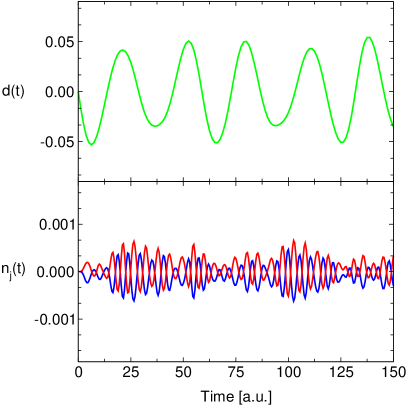
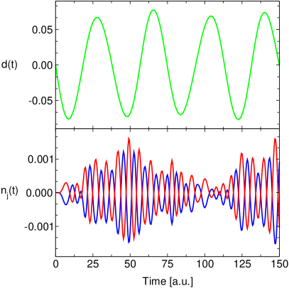
Figure 12: Changes in the dipole moment (green) and the first two natural occupation numbers (red and blue) for the helium atom (left) and the hydrogen molecule (right) in linear response to a $\delta$-kick of strength ${\cal E}_{0}=0.05$ Ha/bohr.

The use of adiabatic approximations in DFT is known to miss certain aspects of the interacting system, one of which being the double excitations discussed in Section 4. Another example are charge-transfer excitations which, while appearing in linear response, are not described correctly [6]. Recently, it has been suggested that using reduced density-matrix functional theory (RDMFT) these problems can be addressed, even within adiabatic approximations [25].

RDMFT uses the one-body density matrix (1RDM)

$$\gamma_{1}({\bf r},{\bf r}^{\prime})=\!N\!\!\int\!\!\!\!\int\!d^{3}r_{2}...d^{3}r_{N}\Psi({\bf r},{\bf r}_{2}...{\bf r}_{N})\Psi^{*}({\bf r}^{\prime},{\bf r}_{2}...{\bf r}_{N})$$ (31)

as its basic variable. Approximations within this theory are usually stated in terms of the eigenfunctions $\varphi_{j}({\bf r})$ and eigenvalues $n_{j}$ of $\gamma_{1}({\bf r},{\bf r}^{\prime})$ which satisfy

$$\int d^{3}r^{\prime}\gamma_{1}({\bf r},{\bf r}^{\prime})\varphi_{j}({\bf r}^{\prime})=n_{j}\varphi_{j}({\bf r})$$ (32)

and are called natural orbitals and occupation numbers, respectively. The exact kinetic energy of a system can be written explicitly in terms of the 1RDM which presents a major advantage compared to standard density functional theory.

Since in general the interaction energy is known as an exact functional of the diagonal $\gamma_{2}({\bf r},{\bf r}^{\prime};{\bf r},{\bf r}^{\prime})$ of the two-body density matrix (2RDM)

$$\gamma_{2}({\bf r}_{1},{\bf r}_{2};{\bf r}^{\prime}_{1},{\bf r}^{\prime}_{2})=\!\frac{N(N-1)}{2}\!\!\int\!\!\!\!\int\!d^{3}r_{3}...d^{3}r_{N}$$ (33)

$$\Psi({\bf r}_{1},{\bf r}_{2},{\bf r}_{3}...{\bf r}_{N})\Psi^{*}({\bf r}^{\prime}_{1},{\bf r}^{\prime}_{2},{\bf r}_{3}...{\bf r}_{N}),$$

RDMFT can be viewed as a way to express the diagonal of the 2RDM as a functional of the 1RDM. Using this functional, the interaction energy is written typically as a sum of the Hartree energy and the exchange-correlation (xc) energy, where only the correlation energy needs to be approximated. Approximations are usually stated by writing either the diagonal of the 2RDM or the xc energy as a functional of the natural orbitals and occupation numbers. For most currently employed functionals the xc energy takes the form [26, 27, 28, 29, 30, 31]

$$E_{xc}[\{\varphi_{j}\},\{n_{j}\}] = -\frac{1}{2}\sum_{j,k=1}^{\infty}f(n_{j},n_{k})$$

$$\times\int\!\!\!\!\int\frac{\varphi_{j}({\bf r})\varphi_{j}^{*}({\bf r}^{\prime})\varphi_{k}({\bf r}^{\prime})\varphi_{k}^{*}({\bf r})}{|{\bf r}-{\bf r}^{\prime}|}d^{3}rd^{3}r^{\prime},$$

i.e. it is given as an exchange integral modified by a function depending on the occupation numbers. Generally, one can expand the 2RDM in the basis of the natural orbitals

$$\gamma_{2}({\bf r}_{1},{\bf r}_{2};{\bf r}^{\prime}_{1},{\bf r}^{\prime}_{2})=\sum_{ijkl}\gamma_{2,ijkl}\varphi_{i}({\bf r}_{1})\varphi_{j}({\bf r}_{2})\varphi_{k}^{*}({\bf r}^{\prime}_{1})\varphi_{l}^{*}({\bf r}^{\prime}_{2}),$$ (35)

which gives rise to expansion coefficients $\gamma_{2,ijkl}$. Restricting these coefficients to the form

$$\gamma_{2,ijkl}=n_{i}n_{j}\delta_{ik}\delta_{jl}-f(n_{i},n_{k})\delta_{il}\delta_{jk},$$ (36)

the diagonal, $\gamma_{2}({\bf r},{\bf r}^{\prime};{\bf r},{\bf r}^{\prime})$, yields the Hartree energy and the xc energy given in Eq. (6).

Currently, an effort is made to extend the static theory in order to describe time-dependent systems. The most straightforward extension is again achieved by employing an adiabatic approximation [32, 33], i.e. the 2RDM at time $t$ is only treated as a functional of the 1RDM at this point in time. Consequently, in Eq. (35), $\gamma_{2}$ aquires a dependence on time $t$ as do the occupation numbers and natural orbitals. For the coefficients of the 2RDM (in the basis of the natural orbitals at time $t$) such an adiabatic approximation amounts to

$$\gamma_{2,ijkl}(t)\!\!\! = \!\!\!g_{ijkl}[\{n_{j}(t)\}]\delta_{ik}\delta_{jl}-h_{ijkl}[\{n_{j}(t)\}]\delta_{il}\delta_{jk}$$ (37)

$$+\lambda_{ijkl}[\{n_{j}(t)\}],$$

where $g_{ijkl}(t)$ and $h_{ijkl}(t)$ are the time-dependent coefficients for the Hartree and exchange-type integrals, respectively. The time-dependent cumulant $\lambda_{ijkl}(t)$ contains all contributions to the 2RDM which are not of Hartree or exchange type. All three coefficients are approximated as functionals of the occupation numbers. Comparing Eqs. (36) and (37) we note, that an adiabatic extension of the currently employed static functionals to the time domain leads to a vanishing cumulant $\lambda$. By inserting Eq. (37) into the equation of motion for the natural occupation numbers [32], we find

$$\begin{split}i\,\partial_{t}n_{k}(t)&=\sum_{ijl}\lambda_{ijkl}(t)\langle ij|v_{\mathrm{int}}|kl\rangle(t)-c.c.,\end{split}$$ (38)

which directly illustrates that adiabatic approximations based on the form of Eq. (36) cause a zero right-hand side and, hence, lead to occupation numbers which are constant in time. While one can imagine this to be a reasonable approximation in some situations, it will generally not be the case. Including an explicit cumulant in the approximation of $\gamma_{2,ijkl}(t)$ leads to occupation numbers which can aquire a true time-dependence, even if one chooses an adiabatic approximation for $\lambda_{ijkl}(t)$.

To assess the quality of the adiabatic approximation in RDMFT quantitatively, we employ again our 1D model. For such model systems with a small number of electrons one can extract the exact 1RDM from the solution of the time-dependent Schrödinger equation of the interacting system, which allows us to explicitly investigate for which situations constant occupation numbers yield a reasonable description. For this purpose, we employ two different two-electron systems, a 1D helium atom and a 1D hydrogen molecule. The external potentials are given by

$$v_{\rm ext}^{\mathrm{He}}(x)\!\!\!\! = \!\!\!\!-\frac{2}{\sqrt{x^{2}+a^{2}}},$$ (39)

$$v_{\rm ext}^{\mathrm{H_{2}}}(x)\!\!\!\! = \!\!\!\!-\frac{1}{\sqrt{(x+d/2)^{2}+a^{2}}}-\frac{1}{\sqrt{(x-d/2)^{2}+a^{2}}}$$ (40)

$$+\frac{1}{\sqrt{d^{2}+a^{2}}},$$

i.e. we are using a soft-Coulomb potential to describe the interaction between the nuclei and the electrons and, for the hydrogen molecule, also the interaction between the two nuclei.

In the following, we investigate two different situations. In the first case we apply a kick, Eq. (9), which provides an initial momentum to the system. We choose the strength ${\cal E}_{0}=0.05$ Ha/bohr such that the evolution can be described in linear response. As a second case, we investigate the transition of the system, here the helium atom, from its ground state to the first excited singlet state. To this end we use optimal control theory [34, 35, 36] to find an optimized laser pulse which induces a transition with a population of the excited state of 98.59% at the end of the pulse.

In Fig. 12, we show the dipole moment and the change in the first two natural occupation numbers, $\Delta n_{j}(t)=n_{j}(t)-n_{j}(t=0)$, for both the helium atom and the hydrogen molecule. The strength of the kick was chosen as the maximum possible while staying within a linear response description. As we can see, the occupation numbers show pronounced oscillations which, however, remain small in amplitude compared to their ground state values while the dipole moment shows the characteristic oscillations. Hence, in linear response, a description with constant occupation numbers will be appropriate.

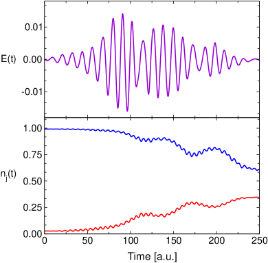
Figure 13: The upper panel displays the laser amplitude of an optimized laser pulse that induces a transition from the ground state to the first excited singlet state of Helium. In the lower panel the two largest occupation numbers of the reduced one-body density matrix are shown as function of time.

As an example where the occupation numbers change significantly, we examine the transition of the helium atom from its singlet ground state to the first excited singlet state which, due to spin, has multi-reference character. The optimized laser pulse which achieves 98.59% of occupation in the excited state after a time of 250 a.u. is shown in Fig. 13. We also show the evolution of the first two natural occupation numbers which starting close to one and zero, respectively, approach each other during the propagation. In this situation, any description which enforces constant occupation numbers will clearly not describe the situation accurately.

To describe a situation where occupation numbers change in time, functionals in RDMFT have to incorporate time-dependent approximations for the cumulant of the reduced two-body density matrix [37]. Possible approaches along these lines could be based on reconstruction approaches for the cumulant of the two-body matrix [30], or alternatively on antisymmetrized geminal power (AGP) wave functions [38], which was proposed recently [32] and will be investigated in a future study.

7 Conclusions and outlook

In this work we aimed to partially unveil the role of electron-correlation in the electron dynamics of systems driven out of equilibrium. To reach this goal, we have used different 1D model systems where we could assess, by comparing with the exact solution, the quality of density and reduced density-matrix functionals in various situations where the system interacts with external time-dependent fields. We looked at both linear and non-linear responses. The 1D ALDA approximation shows the same behavior as its 3D counterpart leading to the well-known underestimation of the ionization potential and a failure to reproduce the excitations to Rydberg states. Also, as has been seen in the past [4, 20], we showed that in the linear response function double excitations do not appear when using adiabatic approximations (exemplified here by using both ALDA and EXX). For the case studied here, where spatial symmetry has been broken and the ground state is a described by a doubly occupied KS orbital, double excitations become visible beyond linear response for the above mentioned adiabatic functionals. In going to the non-linear regime, we demonstrate that the description of Rabi oscillations within all adiabatic functionals leads to a dynamical detuning as the system is driven out of resonance by the changes in the potential due to the changing density associated with the transition during the Rabi oscillation. This manifests itself in a very small population of the excited state in contrast to the exact resonant propagation. Hence, the description of Rabi oscillations provides a very good test case for the development of non-adiabatic functionals.

Within RDMFT adiabatic extensions of commonly employed ground-state functionals lead to constant occupation numbers. This was shown to be a valid description within linear response but it turns out to be a poor approximation in situations where transitions to and among excited states (with possible multi-reference character) take place during the evolution of the system.

In the future, the 1D model systems will be used to improve existing approximations, especially going beyond the adiabatic dependence on the density or the density matrix. Possible routes along these lines include e.g. orbital functionals in TDDFT, or explicit cumulant approximations in time-dependent RDMFT.

The authors thank Michele Casula, Matthieu Verstraete, Miguel Marques, and Xavier Andrade for helpful discussions. We acknowledge support by MICINN (FIS2010-21282-C02-01), ACI-promociona (ACI2009-1036), ”Grupos Consolidados UPV/EHU del Gobierno Vasco” (IT-319-07), and the European Community through e-I3 ETSF project (Contract No. 211956).

References

- [1] E. Runge, E. K. U. Gross, Density-functional theory for time-dependent systems, Phys. Rev. Lett. 52 (1984) 997.
- [2] M. A. L. Marques, C. A. Ullrich, F. Nogueira, A. Rubio, K. Burke, E. K. U. Gross (Eds.), Time-Dependent Density Functional Theory, Vol. 706 of Lecture Notes in Physics, Springer Berlin / Heidelberg, 2006.
- [3] P. Elliott, S. Goldson, C. Canahui, N. Maitra, Perspectives on double-excitations in tddft, arXiv:1101.3379.
- [4] N. T. Maitra, F. Zhang, R. Cave, K. Burke, Double excitations within time-dependent density functional theory linear response, J. Chem. Phys. 120 (2004) 5932.
- [5] N. T. Maitra, K. Burke, C. Woodward, Memory in time-dependent density functional theory, Phys. Rev. Lett. 89 (2002) 023002.
- [6] A. Dreuw, M. Head-Gordon, Failure of time-dependent density functional theory for long-range charge-transfer excited states: The zincbacteriochlorin-bacteriochlorin and bacteriochlorophyll-spheroidene complexes, J. Am. Chem. Soc. 126 (2004) 4007.
- [7] M. Ruggenthaler, D. Bauer, Rabi oscillations and few-level approximations in time-dependent density functional theory, Phys. Rev. Lett. 102 (2009) 233001.
- [8] E. Räsänen, A. Castro, J. Werschnik, A. Rubio, E. K. U. Gross, Optimal laser control of double quantum dots, Phys. Rev. B 77 (2008) 085324.
- [9] K. Burke, J. Werschnik, E. K. U. Gross, Time-dependent density functional theory: Past, present and future, J. Chem. Phys. 123 (2005) 062206.
- [10] M. Petersilka, E. K. U. Gross, Strong-field double ionization of helium: A density-functional perspective, Laser Phys. 9 (1999) 105.
- [11] Q. Su, J. H. Eberly, Model atom for multiphoton physics, Phys. Rev. A 44 (1991) 5997.
- [12] L. Landau, E. Lifschitz, Quantum Mechanics, Butterworth-Heinemann, 1977.
- [13] M. A. L. Marques, A. Castro, G. F. Bertsch, A. Rubio, octopus: a first-principles tool for excited electron-ion dynamics, Comput. Phys. Commun. 151 (2003) 60.
- [14] A. Castro, et al., octopus: a tool for the application of time-dependent density functional theory, Phys. Stat. Sol. B 243 (2006) 2465.
- [15] N. Helbig, J. I. Fuks, M. Casula, M. J. Verstraete, M. A. L. Marques, I. V. Tokatly, A. Rubio, Density functional theory beyond the linear regime: Validating an adiabatic local density approximation, Phys. Rev. A 83 (2011) 032503.
- [16] M. Casula, S. Sorella, G. Senatore, Ground state properties of the one-dimensional coulomb gas using the lattice regularized diffusion monte carlo method, Phys. Rev. B 74 (2006) 245427.
- [17] L. Shulenburger, M. Casula, G. Senatore, R. M. Martin, Spin resolved energy parametrization of a quasi-one-dimensional electron gas, J. Phys. A 42 (2009) 214021.
- [18] U. Fano, Effects of configuration interaction on intensities and phase shifts, Phys. Rev. 124 (1961) 1866.
- [19] U. Fano, J. W. Cooper, Spectral distribution of atomic oscillator strengths, Rev. Mod. Phys. 40 (1968) 441.
- [20] M. Thiele, S. Kümmel, Photoabsorption spectra from adiabatically exact time-dependent density-functional theory in real time, Phys. Chem. Chem. Phys. 11 (2009) 4631.
- [21] J. Fuks, N. Helbig, I. Tokatly, A. Rubio, Non-linear phenomena in time-dependent density-functional theory: What rabi physics can teach us, arXiv:1101.2880.
- [22] D. J. Tannor, Introduction to Quantum Mechanics a time-dependent perspective, University Science books, 2007.
- [23] A. Martin Sanchez, J. Diaz Bejarano, D. Caceres Marzal, Journal of Sound and Vibration 161 (1993) 19.
- [24] M. Thiele, E. K. U. Gross, S. Kümmel, Adiabatic approximation in nonperturbative time-dependent density-functional theory, Phys. Rev. Lett. 100 (2008) 153004.
- [25] K. Giesbertz, K. Pernal, O. Gritsenko, E. J. Baerends, Excitation energies with time-dependent density matrix functional theory: Singlet two-electron systems, J. Chem. Phys. 130 (2009) 114104.
- [26] A. M. K. Müller, Explicit approximate relation between reduced two- and one-particle density matrices, Phys. Rev. A 105 (1984) 446.
- [27] S. Goedecker, C. J. Umrigar, Natural orbital functional for the many-electron problem, Phys. Rev. Lett. 81 (1998) 866.
- [28] M. Buijse, E. J. Baerends, An approximate exchange-correlation hole density as a functional of the natural orbitals, Mol. Phys. 100 (2002) 401.
- [29] O. Gritsenko, K. Pernal, E. J. Baerends, An improved density matrix functional by physically motivated repulsive corrections, J. Chem. Phys. 122 (2005) 204102.
- [30] M. Piris, A new approach for the two-electron cumulant in natural orbital functional theory, Int. J. Quant. Chem. 106 (2006) 1093.
- [31] S. Sharma, J. K. Dewhurst, N. N. Lathiotakis, E. K. U. Gross, Reduced density matrix functional for many-electron systems, Phys. Rev. B 78 (2008) 201103(R).
- [32] H. Appel, E. K. U. Gross, Time-dependent natural orbitals and occupation numbers, EPL (Europhysics Letters) 92 (2010) 23001.
- [33] K. Pernal, K. Giesbertz, O. Gritsenko, E. J. Baerends, Adiabatic approximation of time-dependent density matrix functional response theory, J. Chem. Phys. 127 (2007) 214101.
- [34] S. A. Rice, M. Zhao, Optical Control of Molecular Dynamics, Wiley, New York, 2000.
- [35] M. Shapiro, P. Brumer, Principles of the Quantum Control of Molecular Processes, Wiley, New York, 2003.
- [36] J. Werschnik, E. K. U. Gross, Quantum Optimal Control Theory, J. Phys. B 40 (2007) R175.
- [37] A. J. Coleman, Structure of Fermion Density Matrices, Rev. Mod. Phys. 35 (1963) 668.
- [38] A. J. Coleman, Structure of Fermion Density Matrices. II. Antisymmetrized Geminal Powers, J. Math. Phys. 6 (1965) 1425.