Hydrodynamic models of self-organized dynamics: derivation and existence theory
Abstract
This paper is concerned with the derivation and analysis of hydrodynamic models for systems of self-propelled particles subject to alignment interaction and attraction-repulsion. The starting point is the kinetic model considered in [10] with the addition of an attraction-repulsion interaction potential. Introducing different scalings than in [10], the non-local effects of the alignment and attraction-repulsion interactions can be kept in the hydrodynamic limit and result in extra pressure, viscosity terms and capillary force. The systems are shown to be symmetrizable hyperbolic systems with viscosity terms. A local-in-time existence result is proved in the 2D case for the viscous model and in the 3D case for the inviscid model. The proof relies on the energy method.
1-Université de Toulouse; UPS, INSA, UT1, UTM ;
Institut de Mathématiques de Toulouse ;
F-31062 Toulouse, France.
2-CNRS; Institut de Mathématiques de Toulouse UMR 5219 ;
F-31062 Toulouse, France.
email: pierre.degond@math.univ-toulouse.fr
3- Department of Physics and Department of Mathematics
Duke University
Durham, NC 27708, USA
email: jliu@phy.duke.edu
4-Department of Mathematics
University of Maryland
College Park, MD 20742-4015
email: smotsch@cscamm.umd.edu
5- Department of Mathematics
California State University, Northridge
18111 Nordhoff St
Northridge, CA 91330-8313
email: vladislav.panferov@csun.edu
Acknowledgements: The authors wish to acknowledge the hospitality of Mathematical Sciences Center and Mathematics Department of Tsinghua University where this research was performed. The research of J.-G. L. was partially supported by NSF grant DMS 10-11738.
Key words: Self-propelled particles, alignment dynamics, hydrodynamic limit, diffusion correction, weakly non-local interaction, symmetrizable hyperbolic system, energy method, local well-posedness, capillary force, attraction-repulsion potential
AMS Subject classification: 35L60, 35K55, 35Q80, 82C05, 82C22, 82C70, 92D50.
1 Introduction
The context of this paper is the hydrodynamic limit of a kinetic model for self-propelled particles. The self-propulsion speed is supposed to be constant and identical for all the particles. Therefore, the velocity variable reduces to its orientation. The particle interactions consist in two parts: an alignment rule which tends to relax the particle velocity to the local average orientation and an attraction-repulsion rule which makes the particles move closer or farther away from each other. This model is inspired both by the Vicsek model [28] and the Couzin model [2, 8].
The model studied in this paper is a generalization of the model of [10] with the addition of an attraction-repulsion interaction potential. More importantly, a different scaling is investigated. In this scaling, the non-local effects of the alignment and attraction-repulsion interactions are kept in the hydrodynamic limit and result in extra pressure and viscosity terms. Beyond the statement of the model, the main result of the present paper is a local-in-time existence theorem in the 2D case for the viscous model (when the non-local effects are retained) and in the 3D case for the inviscid model (when the non-local effects are omitted). Both proofs rely on a suitable symmetrization of the system and on the energy method.
There has been an intense literature about the modeling of interactions between individuals among animal societies such as fish schools, bird flocks, herds of mammalians, etc. We refer e.g. to [1, 2, 8, 17] but an exhaustive bibliography is out of reach. Among these models, the Vicsek model [28] has received particular attention due to its simplicity and the universality of its qualitative features. This model is a discrete particle model (or ’Individual-Based Model’ or ’Agent-Based model’) which consists of a time-discretized set of Ordinary Differential Equations for the particle positions and velocities. A time-continuous version of this model and its kinetic formulation are available in [10]. A rigorous derivation of this kinetic model from the time-continuous Vicsek model can be found in [3]. In the present paper, we extend this model by adding an attraction-repulsion force.
Hydrodynamic models are attractive over particle ones due to their computational efficiency. For this reason, many such models have been proposed in the literature [5, 6, 7, 14, 19, 20, 26, 27]. However, most of them are phenomenological. [10] proposes one of the first rigorous derivations of a hydrodynamic version of the Vicsek model (see also [18, 23, 24] for phenomenological derivations). It has been expanded in [11] to account for a model of fish behavior where particles interact through curvature control, and in [12] to include diffusive corrections. Other variants have also been investigated. For instance, [15] studies the influence of a vision angle and of the dependency of the alignment frequency upon the local density. [9, 16] propose a modification of the model which results in phase transitions from disordered to ordered equilibria as the density increases and reaches a threshold, in a way similar to polymer models [13, 21].
The organization of the paper is as follows. In section 2, we introduce the model of self-propelled particles and set up the associated kinetic equation. We then discuss various scalings which lead to the derivation of the studied hydrodynamic models. We introduce four dimensionless parameters in the problem: the scaled interaction mean-free path , the radius of the interaction region , the noise intensity and the relative strength between the attraction-repulsion and the alignment forces . The scaling considered in [10] ignores the attraction-repulsion force and supposes that , . Here, we investigate four different scaling relations.
-
1.
The weakly non-local interaction scaling without noise: , , . The resulting model is a viscous hydrodynamic model with constrained velocity on the unit sphere. For this case, we assume that the solutions of the kinetic equation are monokinetic. We justify this assumption by studying the space homogeneous kinetic model and prove that the solutions converge on the fast time scale to the monokinetic distribution. We also highlight the variational structure of this space homogeneous kinetic model. Note that the scaling assumption is different from the one used in [10]. It corresponds to increasing the size of the interaction region in the microscopic variables by a factor , as . Therefore, more and more non-local effects are picked up in the hydrodynamic limit. These non-local effects give rise to the viscosity terms in the macroscopic models which make an original addition from previous work.
-
2.
The local interaction scaling with noise. This is the scaling proposed in [10] which is recalled here just for the sake of comparisons. It consists in , , . The resulting model is the inviscid hydrodynamic model with constrained velocity on the unit sphere.
-
3.
The weakly non-local interaction scaling with noise. This scaling unifies the two previous scalings. It consists in , , . Again, the resulting model is a viscous hydrodynamic model with constrained velocity on the unit sphere, but with modified coefficients as compared to the first scaling. We note however, that in the zero noise limit , we recover the system obtained with the first scaling, which provides another justification of the monokinetic assumption in the derivation of the model.
-
4.
Capillary force scaling. This corresponds to , , . Therefore, here, the attraction repulsion force is of the same order as the alignment force. However, we make the additional assumption that the zero-th order moment of the potential is zero, which expresses some kind of balance between the attraction and repulsion effects. This results in a model like in the previous scaling, but with the addition of a term analog to the capillary force, induced from the attractive part of the potential.
In section 3, we prove local well-posedness for all the models derived in section 2, except the last one (capillary force scaling). All the remaining systems have the same form of a symmetrizable hyperbolic system with additional viscosity. In section 3.1, we prove the local-in-time existence of solutions for the viscous system in 2D and in section 3.2, we show the same result for the inviscid system in 3D based on the energy method. Finally, a conclusion is drawn in section 4.
2 Derivation of hydrodynamic models
2.1 Individual-Based Model of self-alignment with attraction-repulsion
The starting point of this study is an Individual-Based Model of particles interacting through self-alignment [28] and attraction-repulsion [2, 8]. Specifically, we consider particles moving at a constant speed . Each particle adjusts its velocity to align with its neighbors and to get closer or further away. The evolution of each particle is modeled by the following dynamics:
| (2.1) | |||||
| (2.2) |
Here, is the projection matrix onto the normal plane to :
It ensures that stays of norm . is a Brownian motion and represents the noise intensity. Both the alignment and attraction-repulsion rules are encoded in the vector :
where counts for the alignment and for the attraction-repulsion:
| (2.3) |
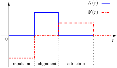
The kernel is a positive function, can be both negative (repulsion) and positive (attraction). In figure 1, we give an example of functions and modeling the popular “zone-based” model for fish behavior [2, 8, 22].
When the number of particles becomes large (i.e. ), one can formally derive the equation satisfied by the particle distribution function (i.e. the probability distribution of the particles in phase-space ). Under suitable assumptions [3, 10, 25], satisfies:
| (2.4) |
where
The function is the antiderivative of which vanishes at infinity (i.e. ). Using the distribution , we want to identify the asymptotic behavior of the model in different regimes. This is the purpose of the next section.
2.2 Scaling parameters
Introducing two dimensionless parameters and , the starting point is the following scaled version of the previous kinetic model for the distribution function :
| (2.5) |
where
| (2.6) | |||
| (2.7) | |||
| (2.8) |
The first term (given by ) expresses the alignment interaction (like in the Vicsek dynamics [28]) while the second term (given by ) expresses the repulsion interaction (like in e.g. [2]). The expression of means that the alignment term will prevail in the limit . In this paper, we will consider various possible assumptions concerning the relative speeds of convergence of and to .
We denote:
We can always assume that . The potential is said to be repulsive if . Defining the moments and of by
we have the following Taylor expansion of :
Inserting this expression into the kinetic equation (2.5), we get
| (2.9) |
We now consider three different scaling limits which lead to models for which we will prove local existence of classical solutions.
2.3 Weakly non-local interaction scaling without noise
In this scaling limit, we assume no noise and the following ordering between the two parameters and :
satisfies (keeping only the terms in or larger):
| (2.10) |
For to converge, we need to assume that the leading order term at the right-hand side of (2.10) vanishes, i.e. that satisfies:
This is equivalent to assuming that is a monokinetic distribution, i.e.
| (2.11) |
where is the delta distribution on the sphere at the point . The assumption of monokinetic distribution requires, in order to be consistent, that there is no noise, which is the reason for assuming .
Proposition 2.1
For monokinetic solutions (2.11), and are independent of and satisfy the following system:
| (2.12) | |||
| (2.13) |
Proof. The result follows from multiplying (2.10) by and and using Green’s formula.
Remark 2.1
The repulsive force contributes for a pressure term at the left-hand side of the momentum equation, which otherwise would not be strictly hyperbolic, and would fall in the class of Pressureless Gas Dynamics models [4].
In order to justify the monokinetic assumption, we consider the spatial homogeneous equation:
| (2.14) |
and show that its solution relaxes to a monokinetic distribution (2.11) at the fast time scale. More precisely, we have
Proposition 2.2
We assume that so that we have for all times. Therefore, (we omit the index when the context is clear). We also assume that , otherwise, the dynamics is not defined. Then, where is of the form .
Proof. We introduce the variance:
We have . We note that is the classical order parameter [28]. In Lemma 2.3 below, we prove that satisfies the following dissipation equation:
| (2.15) |
Since , we have
Therefore, is a decreasing function of time. Furthermore, if is a distribution such that
then, either or is of the form:
where and . The second form is called a dipole. So, unless is a delta or a dipole, is strictly decaying. Since a dipole is unstable, it is never reached in the course of the dynamics. Therefore, as . Since is equivalent to , this shows that as and the typical convergence time is .
Proof. We write
In the last equality, we have used that . Now, multiplying (2.14) by , integrating with respect to and using Green’s formula, we get:
But
which leads to the result.
is a free energy for the problem (2.14) and provides a variational structure. First, let us denote by the gradient of with respect to . It is defined by
where is an increment of , i.e. a function satisfying (so that satisfies the admissibility condition ).
Proposition 2.4
Remark 2.2
Eq. (2.17) provides another proof of the decay of with time.
2.4 Local interaction scaling with noise
In this scaling we assume that . More precisely, we let:
with a given constant. We also assume that and are such that:
With this last assumption, the term in (2.9), which results from the non-locality of the average alignment direction, vanishes. Therefore, this scaling keeps only the local contribution of the alignment interaction. The resulting asymptotic problem, keeping only terms of order or larger, is written:
| (2.18) |
The limit of (2.18) as has been studied in [10] in dimension and in [15] in any dimensions. The result is stated in the following theorem.
Theorem 2.5
We have where is the Von Mises-Fischer distribution:
| (2.19) |
and and satisfy the following system:
| (2.20) | |||
| (2.21) |
The constants and are defined by
where is the Generalized Collision Invariants (GCI) [10] and is defined as follows in the -dimensional case [15]. Set where is any vector such that . Then, is the unique solution in the Sobolev space with zero mean, of the following elliptic problem:
2.5 Weakly non-local interaction scaling with noise
In this section, we propose a scaling which unifies the two previous ones. In this scaling we assume that , with is a given constant and that:
Here instead of like in the previous section. Inserting these assumptions into (2.9), and keeping terms of order or larger, we get
| (2.22) |
The limit is investigated in the following theorem:
Theorem 2.6
Proof. We write (2.22) as
where and are respectively the operators appearing at the left and right hand sides of (2.22). and is the remaining part of the left-hand side. Integrating over and letting leads to the mass conservation equation (2.20) unchanged, since is in divergence form and vanishes through integration with respect to .
Now, to get the momentum equation, we proceed like in [10]. From the Generalized Collision Invariant property [10], it follows that
Now, the term
gives rise to the same expression as in [10]. This expression is
with
Dividing by , we find the coefficients and of (2.21) (we recall that ).
We introduce the notation
and consider
Using Green’s formula, we get
We note that , with being any component of . We deduce that
| (2.26) | |||||
Now, we use the formulas:
for any pair of scalar functions , on . We recall that . Since , we compute the matrix
We decompose
Using this decomposition and the fact that integrals of odd degree polynomials of over vanish, we have:
and
Owing to the fact that any term of the form for any vector , we have since is parallel to :
Inserting these results into (2.26), we get
Collecting all the results and dividing by , we are led to the momentum equation (2.24), which ends the proof.
2.6 Attraction-repulsion potential: induced capillary force
In this section, we investigate the case where the attraction-repulsion force term is of the same order as the alignment term in the expression of the alignment direction , i.e. we assume that
| (2.27) |
where and are respectively given by (2.7) and (2.8). Note that, by contrast to (2.6), there is no in front of in (2.27).
The Taylor expansion of is now given by
where
Here, we suppose like in [2], that the potential is repulsive at short scales and attractive at large scales (See Fig. 2). Therefore, is supposed to decrease for and to increase for . Furthermore, since is supposed integrable on , we have as . It results that and that for and for where . We make the additional assumption that the zero-th order moment vanishes:
which expresses the balance between the attractive and repulsive parts of . Given the above assumptions, the second moment is negative:
With these assumptions, the Taylor expansion of simplifies and becomes:
| (2.28) |
Now, we can develop the same theory as before, assuming that
Inserting these assumptions into (2.9), and keeping terms of order or larger, we get (2.22) but with given by (2.28). The limit can be performed like in section 2.5 and we obtain the following theorem:
Theorem 2.7
Remark 2.4
The last term at the right-hand side of (2.30) has the same expression as the capillary force in fluid dynamics, except for the projection operator . This capillary force is induced from the attractive part of the potential .
3 Existence theory
3.1 Existence in 2D with viscosity
This section is concerned with a local existence result in 2D for a system of the general form
| (3.1) | |||
| (3.2) |
where the constants and are given and the pressure relation satisfies . All systems derived in the previous section can by recast in this form, with a particular choice of , and , after time rescaling, except for the last one (section 2.6) involving the capillary force. The system is supplemented with initial data and such that . We assume that the domain is the square box with periodic boundary conditions.
Theorem 3.1
We assume that the initial data belong to with . Then, there exists a time and a unique solution in such that remains positive. If, in addition, , then, the solution also belongs to .
Proof. In 2D, we can set . We recall that
with . Then, we have
Therefore, system (3.1), (3.2) is written:
| (3.3) | |||
| (3.4) |
Introduce and such that
| (3.5) |
Then, system (3.3), (3.4) becomes:
| (3.6) | |||
| (3.7) |
From (3.6), we have the following a priori estimate (maximum principle):
| (3.8) |
where
We remind the following lemmas [29]:
Lemma 3.2
For any pair of functions , in , we have:
If additionally, we suppose that , we have, for any , with :
where .
Now, with , we take the derivative of (3.6) and multiply it by and integrate it with respect to . Similarly, we take the derivative of (3.7) and multiply it by and integrate it with respect to . We sum up the resulting identities. Using the notation
we find:
Then:
and
where just indicates an norm. Now, for the remaining terms, we have the following lemma
Lemma 3.3
We have:
where denote generic constants depending on the parameters of the problem.
The proof of the lemma is postponed at the end.
Adding all these terms together for all possible indices such that , we have,
For , we have
and get
Gronwall’s inequality leads to the local existence of a solution in which, if , also belongs to and which satisfies the a priori bound (3.8). To get time regularity, we directly use eqs. (3.6), (3.7), take the norm, apply Lemma 3.2, and find
Using the previous estimates, we deduce that also belongs to . The estimates on immediately transfer to since is smooth and invertible for .
Proof of Lemma 3.3. Estimate of : Using Green’s formula and Cauchy-Schwartz inequality, we have:
The second inequality uses Lemma 3.2 and the third one uses Young’s inequality.
Estimate of : We write
Using Green’s formula, we find
Now, using Cauchy-Schwartz inequality and applying Lemma 3.2, we find that and satisfy the same inequality.
Estimate of : The proof is similar as for and is omitted.
3.2 Existence in 3D without viscosity
In this section, we investigate the local existence for the inviscid problem in 3 dimensions:
| (3.9) | |||
| (3.10) |
where the parameters and data have the same meaning as in section 3.1. We consider the system in the domain with periodic boundary conditions.
For this purpose, we use the spherical coordinates associated to a fixed Cartesian basis. In this basis, denoting by the latitude and the longitude, we have
and we let and be the derivatives of with respect to and . We note that
We will use the formulas
where is an arbitrary vector.
Introduce and as in (3.5). Then, system (3.9), (3.10) becomes:
or,
| (3.11) | |||
| (3.12) | |||
| (3.13) |
Introducing
this system is written
in Cartesian coordinates , where , are all symmetric matrices and
If , then this system is a symmetrizable hyperbolic system. We can apply proposition 2.1 p. 425 of [29] and the following theorem follows immediately:
Theorem 3.4
We assume that the initial data belong to with with , . Then, there exists a time and a unique solution in such that remains positive.
4 Conclusion
In this paper, we have derived hydrodynamic systems from kinetic models of self-propelled particles with alignment interaction and attraction-repulsion force. We have particularly focused on the inclusion of diffusion terms under the assumption of weakly non-local interactions. Then, we have proved the local-in-time existence of solutions for the viscous system in 2D and a similar result for the inviscid system in 3D. The methods rely on a suitable symmetrization and on the energy method. Future works in this direction will consist in continuing the exploration of the mathematical structure of the system and particularly, trying to prove local existence of the viscous system in 3D and the treatment of the geometric singularity near . Another direction of work will consist of the numerical quantification of the viscosity as a consequence of the non-locality of the interaction.
References
- [1] M. Aldana, C. Huepe, Phase transitions in self-driven many-particle systems and related non-equilibrium models: a network approach, J. Stat. Phys., 112 (2003), pp. 135–153.
- [2] I. Aoki, A simulation study on the schooling mechanism in fish, Bulletin of the Japan Society of Scientific Fisheries, 48 (1982), pp. 1081–1088.
- [3] F. Bolley, J. A. Cañizo, J. A. Carrillo, Mean-field limit for the stochastic Vicsek model, arXiv preprint 1102.1325.
- [4] F. Bouchut, On zero pressure gas dynamics, in Advances in kinetic theory and computing, Series on Advances in Mathematics for Applied Sciences, Vol 22, World Scientific, 1994, pages 171–190.
- [5] J. A. Carrillo, M. R. D’Orsogna, V. Panferov, Double milling in self-propelled swarms from kinetic theory, Kinetic and Related Models 2, (2009), pp. 363-378.
- [6] J. A. Carrillo, A. Klar, S. Martin, S. Tiwari, Self-propelled interacting particle systems with roosting force, Math. Models Methods Appl. Sci., 20 (2010), pp. 1533-1552.
- [7] Y-L. Chuang, M. R. D’Orsogna, D. Marthaler, A. L. Bertozzi, L. S. Chayes, State transitions and the continuum limit for a 2D interacting, self-propelled particle system, Physica D, 232 (2007), pp. 33–47.
- [8] I. D. Couzin, J. Krause, R. James, G. D. Ruxton, N. R. Franks, Collective Memory and Spatial Sorting in Animal Groups, J. theor. Biol., 218 (2002), pp. 1–11.
- [9] P. Degond, A. Frouvelle, J. G. Liu, Macroscopic limits and phase transition in a system of self-propelled particles, in preparation.
- [10] P. Degond, S. Motsch, Continuum limit of self-driven particles with orientation interaction, Math. Models Methods Appl. Sci., 18, Suppl. (2008), pp. 1193–1215.
- [11] P. Degond, S. Motsch, A Macroscopic Model for a System of Swarming Agents Using Curvature Control, J. Stat. Phys., (2011), available online (DOI 10.1007/s10955-011-0201-3).
- [12] P. Degond, T. Yang, Diffusion in a continuum model of self-propelled particles with alignment interaction, Math. Models Methods Appl. Sci., 20, Suppl. (2010), pp. 1459–1490.
- [13] M. Doi, S. F. Edwards, The theory of polymer dynamics, Clarendon Press, 1999.
- [14] M. R. D’Orsogna, Y. L. Chuang, A. L. Bertozzi, L. Chayes, Self-propelled particles with soft-core interactions: patterns, stability and collapse, Phys. Rev. Lett., 96 (2006), p. 104302.
- [15] A. Frouvelle A continuous model for alignment of self-propelled particles with anisotropy and density-dependent parameters, preprin arXiv 0912.0594.
- [16] A. Frouvelle, J. G. Liu, Dynamics, in a kinetic model of oriented particles with phase transition, preprin arXiv 1101.2380.
- [17] G. Grégoire, H. Chaté, Onset of collective and cohesive motion, Phys. Rev. Lett., 92 (2004) 025702.
- [18] V. L. Kulinskii, V. I. Ratushnaya, A. V. Zvelindovsky, D. Bedeaux, Hydrodynamic model for a system of self-propelling particles with conservative kinematic constraints, Europhys. Lett., 71 (2005), pp. 207–213.
- [19] A. Mogilner, L. Edelstein-Keshet, A non-local model for a swarm, J. Math. Biol., 38 (1999), pp. 534–570.
- [20] A. Mogilner, L. Edelstein-Keshet, L. Bent, A. Spiros, Mutual interactions, potentials, and individual distance in a social aggregation, J. Math. Biol., 47 (2003), pp. 353–389.
- [21] L. Onsager. The effects of shape on the interaction of colloidal particles, Annals of the New York Academy of Sciences, 51 (1949), pp. 627-659.
- [22] J. K Parrish, S. V Viscido, D. Grunbaum Self-organized fish schools: an examination of emergent properties, Biological Bulletin, Marine Biological Laboratory, Woods Hole (2002), pp. 296–305
- [23] V. I. Ratushnaya, D. Bedeaux, V. L. Kulinskii, A. V. Zvelindovsky, Collective behaviour of self propelling particles with kinematic constraints ; the relations between the discrete and the continuous description, Physica A, 381 (2007), pp. 39–46.
- [24] V. I. Ratushnaya, V. L. Kulinskii, A. V. Zvelindovsky, D. Bedeaux, Hydrodynamic model for the system of self propelling particles with conservative kinematic constraints; two dimensional stationary solutions Physica A, 366 (2006), pp. 107–114.
- [25] A. S Sznitman, Topics in propagation of chaos, École d’été de probabilités de Saint-Flour XIX-1989. Lecture Notes in Math, 1464:165–251, 1989.
- [26] C. M. Topaz, A. L. Bertozzi, Swarming patterns in a two-dimensional kinematic model for biological groups, SIAM J. Appl. Math, 65 (2004), pp. 152–174.
- [27] C. M. Topaz, A. L. Bertozzi, M. A. Lewis, A nonlocal continuum model for biological aggregation, Bull. Math. Biol., 68 (2006), pp. 1601–1623.
- [28] T. Vicsek, A. Czirók, E. Ben-Jacob, I. Cohen, O. Shochet, Novel type of phase transition in a system of self-driven particles, Phys. Rev. Lett., 75 (1995), pp. 1226–1229.
- [29] M. E. Taylor, Partial Differential Equations III, Applied Mathematical Sciences Series Vol. 117, Springer, 1996, 2011.
- [30] V. Villani, Topics in optimal transportation, AMS Graduate Studies in Mathematics, Vol. 58, AMS, Providence, 2003.