The focusing effect of cold atomic cloud with a red-detuned Gaussian beam

Abstract

We have demonstrated an atom-optical lens, with the advantage of a small scale and flexible adjustment of the parameters, realized by a far red-detuned Gaussian laser beam perpendicular to the propagation direction of the cold atomic cloud. The one-dimensional transverse focusing effect of cold atomic clouds at the temperature order of 1 $\mu$K freely falling through the atom-optical lens on the micron scale have been studied theoretically and then verified experimentally. It is found that theory and experiment are in good agreement.

I Introduction

An atom-optical lens is one of the fundamental atom-optical elements, which can focus, collimate, image and transmit the atom beam or atomic cloud Meystre ; PR240-143 . Up to now two main types of atom-optical lens, based on magnetic or optical fields, have been developed. Atom-optical lenses based on magnetic fields PRL67-2439 ; PRL87-030401 ; PRA65-031601 ; APB2007 are advantageous for coherent atom-optics research owing to their extremely high optical quality. However, it is difficult to build flexible optical systems because magnetic atom-optical elements have a large scale. In contrast, atom-optical lens based on the optical dipole force has a small scale and is flexible to realize the combination of atom-optical lenses PR240-143 ; BFAP78 ; JOSAB8-502 . Except for optical dipole force, radiation-pressure force Wpzhang1 ; Wpzhang2 ; JETP43-217 ; JMO35-17 , near-field light JOA8-153 ; PRA77-013601 , and far-detuned and resonant standing wave fields PRA60-4886 are also utilized to realize an atom-optical lens.

Focusing of an atomic beam or cloud are one of most important applications of atom-optical lens, which can offer high bright sources. Such sources are desired by atom lithographylith , atom interferometry, atomic fountain clockclock , atomic physics collision experimentscollision , ultra high resolution optical spectrum and quantum frequency standard. In fact, all these applications of atom-optical lens do not require a small scale. However, when considering loading or transmitting atomic cloud onto micro-trap or micro-waveguide on a integrated atom chip, the atom-optical lenses on the micron scale are expected. For a Gaussian laser beam with red detuning, the dipole force is toward the maximum intensity region. Hence, a focused Gaussian laser beam with red detuning can be used as an atom-optical lens. To avoid the aberration of the atom-optical lens from the spontaneous emission, the detuning should be large enough. Experimentally, the waist of the focused laser beam can be focused to several microns. Consequently, a focused red-detuned Gaussian laser beam is suitable to make the atomic beam or cloud focus on the micron scale.

In our previous work we have experimentally observed focusing and advancement effects when ultracold atomic clouds and BEC wave packets passed through focused red-detuned Gaussian laser beamPRA80-033411 . In that work the dynamics of ultracold cloud and BEC are described by the linear (nonlinear) Schordinger equation. While this work will theoretically study the one-dimensional focusing of cold atomic clouds passing through an atom-optical lens with Newtonian mechanics and then experimentally verify the theoretical prediction. The atom-optical lens suggested in this work has the advantage of easily constructing and aligning the setup because the laser beam is perpendicular to the propagation direction of the atomic cloud.

The remainder of the paper is organized as follows. In Sec. II we study the focusing of the atom-optical lens induced by far red-detuned Gaussian laser beam using particle tracing method when the atom is under gravity field. In Sec III the experimental investigation of the focusing effects is presented and discussed. Finally we conclude the work.

II Theory analysis

We first consider an atom located at the position $(0,0,L)$ freely falling along $z$ axes to a potential induced by a far red-detuned focused Gaussian laser beam:

$$U=-U_{0}\exp\left(-\frac{y^{2}+z^{2}}{\sigma_{0}^{2}}\right),$$ (1)

where interaction intensity $U_{0}=\hslash\Omega^{2}/4\left|\delta\right|$. Here $\Omega$ is determined by the intensity in the center of the Gaussian beam, and $\sigma_{0}$ is the waist width of the Gaussian beam. $\delta=\omega_{L}-\omega_{a}$ presents the detuning between the laser frequency and the transition frequency of the atom. When the detuning is red, the potential is negative and presents an attractive force when the atoms passing through it. The red-detuned Gaussian laser beam can therefore serve as a focal cylindrical atom-optical lens. To avoid the aberration of the atom-optical lens from the spontaneous emission, the detuning $\delta$ should be far larger than the spontaneous emission rate.

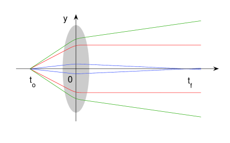
Figure 1: (Color online) Space-time diagram of the atomic trajectory. The object point is focused on imaging point by the atom lens.

Now we will investigate the focusing effect of the atom-optical lens by solving the motion equation of atoms:

$$m\frac{d^{2}\vec{r}}{dt^{2}}=-\vec{\nabla}\left(U-mgz\right),$$ (2)

where $m$ is the atom mass. Due to free expansion of the atomic cloud along $x$ direction, hereafter we will denote $y$ direction as transverse direction.

We assume that, without loss of important physics, the initial height of the atoms is sufficiently large so that, when atoms pass through the laser beam, their kinetic energies are far greater than the optical potential, and therefore their velocity along $z$ direction almost remains unchanged moment . Under this assumption, we obtain the transverse momentum change along $y$ direction on the atomic center of mass can be found with the law of impulse-momentum

$$m\Delta v_{y} = -\int_{-\infty}^{\infty}\frac{\partial}{\partial y}U\left(t\right)dt$$ (3)

$$\simeq mv_{y0}f$$

with

$$f=-\frac{2\sqrt{\pi}U_{0}}{mg\sigma_{0}}\exp\left(-\frac{v_{y0}^{2}t_{o}^{2}}{\sigma_{0}^{2}}\right)$$ (4)

where $t_{o}=\sqrt{2L/g}$ is the falling time spent by the atom to reach the center plane of the laser beam from its initial position and $v_{y0}$ is its initial transverse velocity.

Using the simple geometric relationship of time-space trajectories of atoms, as shown in figure 1, one finds that the relation between flying time $t_{o}$ and the focusing time $t_{f}$ in imaging region as

$$t_{f}=-\frac{t_{o}}{\left(f+1\right)}$$ (5)

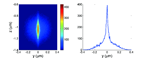
Figure 2: (Color online) The simulation of focusing atomic clouds by the Gaussian laser beam. (a) shows images of the simulated cold atomic cloud passing through the laser beam. (b) is the corresponding cross section of focused atomic cloud along $y$ direction at the widest part of atomic cloud. The initial temperatures of the atomic clouds is $0.5\mu$ k. The flying times of the atomic cloud are $t_{0}=7$ ms and $t=10$ ms. Other parameters are $U_{0}=3.0\times 10^{-29}$J and $\sigma_{0}=50\mu m$.

From Eq. (5) one can note that, if $f<-1$, $t_{f}>0$, the atomic trajectory will be bent to the axes of the atomic lens in the imaging region, i.e., a real image of the atom formed by the atomic lens; if $f>-1$, $t_{f}<0$, the atomic trajectory will be bent from the axes in imaging region. Hence the dimensionless parameter $f$ characterizes the the atom deflection by the laser beam. Eq. (4) suggests that the parameter $f$ can be easily controlled by adjusting the interaction intensity $U_{0}$ or the laser beam waist $\sigma_{0}$, and therefore one can focus or defocus the atomic cloud by adjusting the parameters of the laser beam.

Eq. (5) also shows that the time for the atomic cloud to be focused after it passes through the laser beam is proportional to the initial flying time, which is different from the ordinary object-image relationship of focal atom-optical lens in the time domain PRA59-4636 . This is because the atoms are accelerated in gravity in our case while the velocity is uniform in other cases. Additionally, from Eqs. (5) and (4) one can find that the focusing time is dependent on the initial transverse velocity of the atom. Consequently, an atomic cloud will be focused to one small spot, instead of one point. This leads to the spherical aberration of the atom-optical lens.

Now we consider the case of cold atomic ensemble. Since the parameter $f$ is dependent on the transverse velocities of the atoms, the atoms in the ensemble may be focused or not by the atomic lens dependent on its initial transverse velocity. Figure 1 presents some typical atomic trajectories with different initial transverse velocities. From figure 1 one can see that only the atoms whose initial transverse velocity is smaller than critical velocity $v_{c}$ can be focused in the imaging region by the atomic lens. The critical velocity is determined by

$$f=-1$$ (6)

and the corresonding velocity is

$$v_{c}=\frac{\sigma_{0}}{t_{0}}\sqrt{\ln\left(\frac{2\sqrt{\pi}U_{0}}{mg\sigma_{0}}\right)}.$$ (7)

Eq. (7) shows that, for real experimental parameters, the critical velocity has a finite maximum value, in other words, only part of the atoms can be focused. We have numerically simulated the partially focusing effect with a cold atomic cloud passing through the laser beam. From figure 2 we can see that there is a sharply focused peak on the wide unfocused atomic cloud background. Since the focusing effect only happens along $y$ direction, the atomic cloud looks like a long cigar.

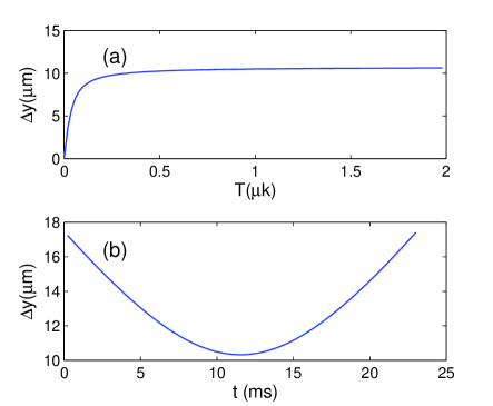
Figure 3: (Color online) The transverse width of peak of the focused atomic cloud dependent on (a) the initial temperature with $t=10$ ms and (b) the falling time with $T=1.0$ $\mu$k. Other parameters are $U_{0}=2.81\times 10^{-29}$J, $\sigma_{0}=35\mu m$ and $t_{o}=7$ms.

Now we calculate the transverse width of the peak of focused atomic cloud along $y$ direction. We assume that the atomic cloud with initial temperature $T$ is released at the position ($0,0,gt_{o}^{2}/2$), it reaches the center of the laser beam after time $t_{o}$ and then to the image region after time $t$. Therefore the half width of the focused atomic cloud in the image region is

$$\Delta y^{2} =\left\langle v_{y}^{2}\left(t_{f}-t\right)^{2}\right\rangle-\left\langle v_{y}\left(t_{f}-t\right)\right\rangle$$

$$=A\int_{-v_{c}}^{v_{c}}v_{y_{0}}^{2}\left(tf+t+t_{o}\right)^{2}\exp\left(-\frac{mv_{y_{0}}^{2}}{2k_{B}T}\right)\,\mathrm{d}v_{y_{0}}$$

$$=\frac{Af_{0}^{2}t^{2}}{2C_{1}^{3}}\left(-2v_{c}C_{1}e^{-v_{c}^{2}C_{1}^{2}}+\sqrt{\pi}\mathrm{Erf}\left(v_{c}C_{1}\right)\right)$$

$$+\frac{2Af_{0}t\left(t+t_{o}\right)}{2C_{2}^{3}}\left(-2v_{c}C_{2}e^{-v_{c}^{2}C_{2}^{2}}+\sqrt{\pi}\mathrm{Erf}\left(v_{c}C_{2}\right)\right)$$ (8)

$$+\frac{A\left(t+t_{o}\right)^{2}}{2C_{3}^{3}}\left(-2v_{c}C_{3}e^{-v_{c}^{2}C_{3}^{2}}+\sqrt{\pi}\mathrm{Erf}\left(v_{c}C_{3}\right)\right)$$

with

$$C_{1} =\sqrt{\frac{2t_{o}^{2}}{\sigma_{0}^{2}}+\frac{t_{o}^{2}}{\sigma_{a}^{2}}}$$ (9a)

$$C_{2} =\sqrt{\frac{t_{o}^{2}}{\sigma_{0}^{2}}+\frac{t_{o}^{2}}{\sigma_{a}^{2}}}$$ (9b)

$$C_{3} =\frac{t_{o}}{\sigma_{a}}$$ (9c)

and

$$f_{0}=\frac{2\sqrt{\pi}U_{0}}{mg\sigma_{0}}$$ (10)

where the normalized constant $A=t_{o}/\left(\sigma_{a}\sqrt{\pi}\mathbf{Erf}\left(v_{c}t_{o}/\sigma_{a}\right)\right)$ and the size of the atomic cloud when it reaches the laser beam center $\sigma_{a}^{2}=2t_{o}^{2}k_{B}T/m$ with Boltzmann constant $k_{B}$.

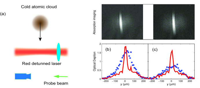
Figure 4: (Color online) The focusing of atomic clouds by the Gaussian laser beam. (a) is the schematic diagram of experimental setup. Top panels of (b) and (c) are the absorption imaging of the focused atomic clouds. The bottom panels are the corresponding cross section of optical depth. The solid lines denote the the focused atomic clouds, while the symbol $\blacksquare$ represent the reference ones. The initial temperatures of the atomic clouds are (a) 190nk and (b) 370nk respectively. The atomic clouds flies 7 ms before they get to the center of laser beam and then 9 ms to the imaging region. Other parameters are $U_{0}=2.81\times 10^{-29}$J and $\sigma_{0}=35\mu m$.

We plot the transverse width of the peak of the focused atomic as functions of initial temperature $T$ and falling time $t$, shown in figure 3, respectively. It can be noted that, from Fig. 3(a), the transverse width is first rapid increases and then approximately approaches to a constant with increasing the initial temperature. Mathematically, this can be seen from Eq. 8 that, when $T$ is very small, $\Delta y^{2}\propto\sigma_{a}^{2}\propto T$, while $T$ is very large, $\Delta y^{2}\propto\exp\left(-mv_{y_{0}}^{2}/\left(2k_{B}T\right)\right)\rightarrow 1$, i.e., $\Delta y$ is independent on $T$. Physically, when the initial temperature of the atomic cloud is very lower, almost all the atoms are focused by the laser beam, and in this case the transverse chromatic aberration dominantly contributes to the transverse width of the focused atomic cloud. When the initial temperature is very high, only the center part of the atomic cloud overlaps the laser beam and is focused by it. The focused atoms tends to be monochromatic, rather chromatic, with increase of the initial temperature. In this situation, the spherical aberration of the atomic lens dominantly contributes to transverse width of the atomic cloud than the transverse chromatic aberration does. Therefore the transverse width is just related with parameters of the atomic lens, instead of the initial temperature of the atom cloud.

When fixing the initial temperature $T$ and changing the falling time $t$, the width of the focused atomic cloud is first decreasing and then increasing, as shown in figure 3(b). The minimum width of the focused atomic cloud along $y$ direction increases with increasing the initial temperature. Of course, if the initial temperature is so lower that the atomic cloud is condensed, the quantum mechanics model is required to describe the focusing effect.

III Experimental result and discussion

Our experimental setup consists of two magneto-optical traps PRA80-033411 . The atomic cloud is firstly captured in the Up-MOT and then transferred into the second ultrahigh-vacuum MOT(UHV-MOT). After the atomic number in the UHV-MOT is stable, we prepared optical molasses and then loaded atoms into a quadrupole-Ioffe-configuration (QUIC) trap. Evaporative cooling of the atoms was performed by rf-induced spin flips. We swept the rf frequency from 25MHz to a value of around 1.6MHz over a period of 28s. Atomic clouds with various temperatures from about 1$\mu$K to below the phase transition point were obtained by setting different rf frequencies. The cold atomic cloud then ballistically expanded after the magnetic trap was switched off. The direction of propagation of the focused Gaussian beam and the probing beam was parallel to the long axis of the QUIC trap. Therefore, the cold atomic clouds symmetrically distributed in the probing plane before traversing the Gaussian beam. We acquired the distribution of atomic clouds from absorption images, as shown schematically in figure 4(a). The Rayleigh length was about 8.5mm. Since the Rayleigh length was far greater than the scale of the atomic cloud while it was passing the light beam, we could approximate that the laser beam provided a two-dimensional Gaussian potential. The power of the focused Gaussian light beam was between $40\sim 45$ $\mu$w with a red detuning $\delta/2\pi=-40\sim-80$ GHz. When evaporative cooling was finished, we released the atomic cloud from the QUIC trap and turned on the Gaussian beam. After the atomic cloud had passed through it, we turned off the Gaussian beam and waited for several milliseconds. All information regarding the atomic cloud was derived from the absorption images.

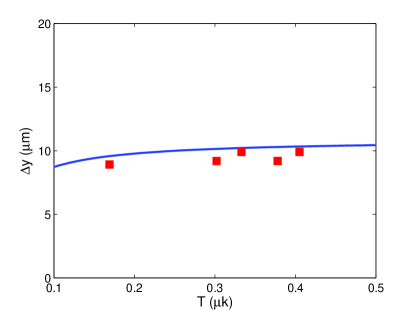
Figure 5: (Color online) The transverse width of the focused part of the atomic cloud against the initial temperature. The symbol $\blacksquare$ gives the experimental result. The solid line is the analytical result. Other parameters are $U_{0}=2.81\times 10^{-29}$J, $\sigma_{0}=35\mu m$, $t_{0}=7ms$, $t=9ms$.

Figures 4(b) and 4(c) are typical experimental results about the focusing of the atomic clouds with different initial temperatures passing through the laser beam. From absorption images and cross section of optical depth we can see that the atomic clouds are focused by the laser beam compared to the reference one. As expected, the focusing just happened along $y$ direction, while the vertical direction remained unchanged. Owing to the finite action length of the laser beam, only the center part of the atomic cloud is focused, which is consistent with our theoretical anlysis. The ratio of focused parts increases with the decrease in temperature.

As the case in figure 3, we also measured the transverse width of the focused part of the atomic cloud with respect to the initial temperature of the atomic cloud and falling time after the focused atomic cloud passing through the laser beam, respectively. The experimental results are plotted in figures 5 and 6, which are well consistent with the analytical prediction.

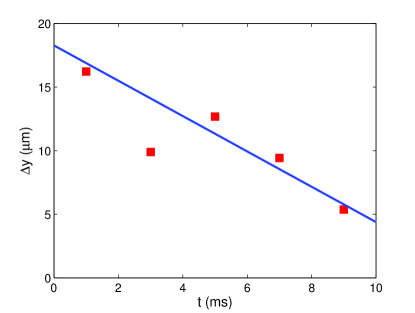
Figure 6: (Color online) The transverse width of the focused part of the atomic clouds plotted against the falling time. The symbol $\blacksquare$ gives the experimental result. The solid line is the analytical result. Before passing through the Gaussian beam, the atomic clouds have already flown 7 ms. Other parameters are $U_{0}=1.26\times 10^{-29}$J, $\sigma_{0}=17\mu m$ and $T_{0}=71nk$.

IV Conclusion

We study the one dimensional transverse focusing effect of an atomic cloud freely falling and passing through the atom-optical lens induced by the far red-detuned laser beam. Based on the atom deflection in dipole conservative potential, the relation between initial falling time and focusing time is theoretically presented. Moreover, atom-optical lens induced by the laser beam has the advantages of small scale and flexible adjustment. It may play an important role in many fields such as, integrated atom optics and atomic fountain clock. Finally we have experimentally demonstrated the focusing, imaging of the atomic cloud passing through the Gaussian laser beam, which are well consistent with the theoretical prediction.

This work is supported by the National Natural Science Foundation of China under Grant Nos. 10828408, 10804115 and 10974211, National Fundamental Research Program of China under Grant No. 2011CB921504.

References

- (1) P. Meystre Atom Optics, Springer-Verlag New York (2001).
- (2) C.S. Adams, M.Sigel and J.Mynek Phys. Rep., 240 143 (1994).
- (3) E.A. Cornell, C. Monroe and C.E. Wieman, Phys. Rev. Lett., 67 2439(1991).
- (4) I. Bloch, M. Köhl, M.Greiner, T.W. Hänsch and T. Esslinger, Phys. Rev. Lett., 87 030401 (2001).
- (5) A.S. Arnold, C.MacCormick and M.G. Boshier, Phys. Rev. A, 65 031601 (2002).
- (6) R. R. Chaustowski, V. Y. F. Leung and K. G. H. Baldwin, Appl. Phys. B 86 491 (2007).
- (7) J.E. Bjorkholm, R.R. Freeman, A. Ashkin and D.B. Pearson, Phys., Rev. Lett. 41 1361 (1978).
- (8) G.M. Gallatin and P.L. Gould, J. Opt. Soc. Am. B, 8 502(1991).
- (9) Heping Zeng, Weiping Zhang, and Fucheng Lin, Phys. Rev. A, 52, 2155(1995).
- (10) Lu Zhou, Weiping Zhang, Hong Y. Ling, Lei Jiang, and Han Pu, Phys. Rev. A, 75, 043603(2007).
- (11) V.I. Balykin, V.S. Letokhov and A.I. Sidorov, JETP. Lett., 43 217 (1986).
- (12) V.I. Balykin et al., J. Mod. Opt., 35 17 (1988).
- (13) H. Ito K. Yamamoto A. Takamizawa H. Kashiwagi and T. Yatsui, J. Opt. A: Pure Appl.Opt., 8 S153 (2006).
- (14) V.I. Balykin and V.G. Minogin,Phys. Rev. A, 77 013601 (2008).
- (15) J.L. Cohen, B. Dubetsky and P.R. Berman, Phys. Rev. A, 60 4886 (1999).
- (16) G. Timp et al., Phys. Rev. Lett., 69 1636 (1992).
- (17) S.R. Jefferts et al., Metrologia, 39 321 (2002).
- (18) W. DeGraffenreid, J. Ramirez-Serrano, Y.-M. Liu and J. Weiner, Rev. Sci. Instrum., 71 3668 (2002).
- (19) S. Y. Zhou, Z. L. Duan, J. Qian, Z. Xu, Weiping Zhang and Y. Z. Wang, Phys. Rev. A, 80 033411 (2009).
- (20) E. Marechal, S. Guibal, J.-L. Bossennec, R. Barbe, J.-C. Keller, and O. Gorceix, Phys. Rev. A, 59 4636 (1999).
- (21) T. Sleator T. Pfau V. Balykin and J. Mlynek, Appl. Phys. B, 54 375 (1992).