Gutzwiller Method for an Extended Periodic Anderson Model
with the $c$-$f$ Coulomb Interaction

Abstract

We study an extended periodic Anderson model with the Coulomb interaction $U_{cf}$ between conduction and $f$ electrons by the Gutzwiller method. The crossovers between the Kondo, intermediate-valence, and almost empty $f$-electron regimes become sharper with $U_{cf}$, and for a sufficiently large $U_{cf}$, become first-order phase transitions. In the Kondo regime, a large enhancement in the effective mass occurs as in the ordinary periodic Anderson model without $U_{cf}$. In addition, we find that a large mass enhancement also occurs in the intermediate-valence regime by the effect of $U_{cf}$.

1 Introduction

In rare-earth and actinide compounds, several interesting phenomena, such as magnetism, heavy-fermion phenomena, and superconductivity, occur owing to the interplay of the strong Coulomb interaction $U$ between $f$ electrons and the hybridization $V$ between the localized $f$-orbital and conduction band.

Among such phenomena, heavy-fermion superconductivity has been one of the central issues in $f$-electron physics after the discovery of the superconductivity in CeCu₂Si₂. [1] In the heavy-fermion systems, the conventional, phonon-mediated, $s$-wave superconductivity is hardly realized owing to the strong onsite Coulomb interaction. Then, pairing mechanisms other than the phonon-mediated mechanism have been discussed. The magnetic-fluctuation-mediated superconducting mechanism may be common in heavy-fermion superconductors, since superconductivity is realized near a magnetic quantum critical point in many compounds.

However, some heavy-fermion superconductors are difficult to understand solely by the magnetic fluctuation scenario. For example, the superconducting transition temperatures under pressure in CeCu₂Si₂ [2] and CeCu₂Ge₂,[3] become maximum far away from the magnetic quantum critical points. In CeCu₂Si_1.8Ge_0.2, [4] the superconducting region splits into two regions: the low-pressure region close to the magnetic critical point and the high-pressure region away from the magnetic critical point. To explain the high-pressure superconducting phase, a valence fluctuation scenario is proposed [5, 6, 7, 8] and the importance of the Coulomb interaction $U_{cf}$ between conduction and $f$ electrons has been discussed in addition to $U$ and $V$.

Valence fluctuations are expected from the rapid change in the valence of an $f$ ion in these compounds under pressure, which is suggested from the behavior of the effective mass $m^{*}$. In the periodic Anderson model (PAM), $m^{*}$ and the number of electrons, $n_{f}$, in the $f$ orbital per site follow the relation [9, 10]

$$\frac{m^{*}}{m}=\frac{1-n_{f}/2}{1-n_{f}},$$ (1)

where $m$ is the free-electron mass. This relation is derived using the Gutzwiller method for $U\rightarrow\infty$. Thus, a large change in $m^{*}$ indicates a large change in $n_{f}$. For CeCu₂Si₂ and CeCu₂Ge₂, $m^{*}$ is experimentally deduced from specific heat measurements or the temperature dependence of electrical resistivity, and it is found that $m^{*}$ decreases rapidly at approximately the pressure where the superconducting transition temperature becomes maximum. [11, 12] Thus, these observations indicate that a sharp valence change or large valence fluctuations play important roles in superconductivity.

However, there are problems with the relation between the effective mass and valence. First, eq. (1) is derived for an ordinary PAM, which does not show a sharp valence change. Thus, we cannot naively apply eq. (1) to a system with large valence fluctuations. Second, the effective mass has a peak in CeCu₂Si₂ under pressure before the superconducting transition temperature becomes maximum, that is, the effective mass varies nonmonotonically under pressure. [12] This nonmonotonic variation in the effective mass cannot be explained by eq. (1), since the $n_{f}$ of a Ce ion is expected to decrease monotonically under pressure for the following reasons. A positively charged Ce ion should be surrounded by negative charges. When these negative charges get close to a Ce ion under pressure, the $f$ level $\epsilon_{f}$ of Ce is lifted. Under pressure, the overlap between the wave functions of the $f$ orbital and the conduction band increases, and $V$ increases. Both the effects of pressure on $\epsilon_{f}$ and $V$ result in a decrease in $n_{f}$. Indeed, a monotonic decrease in $n_{f}$ under pressure has been observed in CeCu₂Si₂ by an X-ray absorption experiment recently. [13] We also note that, in CeCu₂Ge₂, the pressure dependence of the effective mass has a shoulder structure before the superconducting transition temperature becomes maximum. [11] This shoulder structure may also become a peak as in CeCu₂Si₂, if we subtract the contributions of magnetic fluctuations, which are large in the low-pressure region.

The peak structures in the effective mass may be explained by considering a combined effect of the renormalization described by eq. (1) and valence fluctuations. [12] However, the applicability of eq. (1) to a system with large valence fluctuations is not justified. Thus, it is an interesting problem how eq. (1) can be extended to a model that shows a sharp valence change. A study of such a problem will be helpful to understand superconductivity in CeCu₂Si₂ and CeCu₂Ge₂ by the valence fluctuation scenario.

Note that heavy-fermion behaviors in $\alpha$-YbAlB₄ and $\beta$-YbAlB₄ [14] are also difficult to explain by eq. (1). The valences of the Yb ion are $+2.73$ for $\alpha$-YbAlB₄ and $+2.75$ for $\beta$-YbAlB₄, [15] that is, the hole numbers of Yb ions are $n_{f}=0.73$ and 0.75 for $\alpha$-YbAlB₄ and $\beta$-YbAlB₄, respectively. For these values of $n_{f}$, i.e., much less than unity, we cannot expect heavy-fermion behavior from eq. (1).

In this research, we study an extended periodic Anderson model (EPAM) with the Coulomb interaction $U_{cf}$ between conduction and $f$ electrons by the Gutzwiller method. We extend the Gutzwiller method for the PAM developed by Fazekas and Brandow [10] to the present model. Then, we investigate the effect of $U_{cf}$ on the effective mass. Although the EPAM has been studied as a typical model for valence transition [16] and has been investigated by some modern techniques in recent years [6, 17, 7, 8, 18, 19] after the proposal of the valence fluctuation scenario for superconductivity, the effect of $U_{cf}$ on the mass enhancement has not been clarified well. Some of the results have already been reported in our previous paper; [20] here, we report the details of the method and also add new results.

2 Formulation

The EPAM is given by [16]

$$\begin{split}H=&\sum_{\mib{k}\sigma}\epsilon_{\mib{k}}c^{\dagger}_{\mib{k}\sigma}c_{\mib{k}\sigma}+\epsilon_{f}\sum_{\mib{r}\sigma}n_{f\mib{r}\sigma}\\ &-V\sum_{\mib{k}\sigma}(f^{\dagger}_{\mib{k}\sigma}c_{\mib{k}\sigma}+c^{\dagger}_{\mib{k}\sigma}f_{\mib{k}\sigma})\\ &+U\sum_{\mib{r}}n_{f\mib{r}\uparrow}n_{f\mib{r}\downarrow}+U_{cf}\sum_{\mib{r}\sigma\sigma^{\prime}}n_{c\mib{r}\sigma}n_{f\mib{r}\sigma^{\prime}},\end{split}$$ (2)

where $c_{\mib{k}\sigma}$ and $f_{\mib{k}\sigma}$ are the annihilation operators of conduction and $f$ electrons, respectively, with the momentum $\mib{k}$ and the spin $\sigma$. $n_{c\mib{r}\sigma}$ and $n_{f\mib{r}\sigma}$ are the number operators at site $\mib{r}$ with $\sigma$ of the conduction and $f$ electrons, respectively. $\epsilon_{\mib{k}}$ is the kinetic energy of the conduction electron. We have not taken orbital degrees of freedom into consideration. This simplification may be justified for a system with tetragonal symmetry such as CeCu₂Si₂ and CeCu₂Ge₂ and for a system with orthorhombic symmetry such as $\alpha$-YbAlB₄ and $\beta$-YbAlB₄, since the crystalline electric field ground states of $f$ electrons are Kramers doublets in these systems. In the following, we set the energy level of the conduction band as the origin of energy, i.e., $\sum_{\mib{k}}\epsilon_{\mib{k}}=0$. We set $U\rightarrow\infty$, since the onsite Coulomb interaction between well-localized $f$ electrons is large.

We consider the variational wave function given by

$$|\psi\rangle=P_{ff}P_{cf}|\phi\rangle,$$ (3)

where

$$P_{ff}=\prod_{\mib{r}}[1-n_{f\mib{r}\uparrow}n_{f\mib{r}\downarrow}]$$ (4)

excludes the double occupancy of $f$ electrons at the same site, and

$$P_{cf}=\prod_{\mib{r}\sigma\sigma^{\prime}}[1-(1-g)n_{c\mib{r}\sigma}n_{f\mib{r}\sigma^{\prime}}]$$ (5)

is introduced to deal with the onsite correlation between conduction and $f$ electrons. [17] $g$ is a variational parameter. The one-electron part of the wave function is given by

$$|\phi\rangle=\prod_{k<k_{\text{F}},\sigma}[c^{\dagger}_{\mib{k}\sigma}+a(\mib{k})f^{\dagger}_{\mib{k}\sigma}]|0\rangle,$$ (6)

where $k_{\text{F}}$ is the Fermi momentum for the free conduction band without $f$ electrons, $|0\rangle$ denotes vacuum, and $a(\mib{k})$ is determined variationally. Here, we have assumed that the total number $n$ of electrons per site is less than 2.

In the method by Fazekas and Brandow, [10] the $f$-electron state is expanded in the basis state in real space, since it is convenient to deal with the projection operator $P_{ff}$. In the present study, we consider $P_{cf}$ in addition to $P_{ff}$, and thus we also expand the conduction-electron state in real space. This is the main difference from the method of Fazekas and Brandow. The creation operator is expanded as

$$b^{\dagger}_{\mib{k}}=\frac{1}{\sqrt{L}}\sum_{\mib{r}}e^{i\mib{k}\cdot\mib{r}}b^{\dagger}_{\mib{r}}=\sum_{\mib{r}}\varphi_{\mib{k}}(\mib{r})b^{\dagger}_{\mib{r}},$$ (7)

where $L$ is the number of lattice sites and $b$ denotes $c_{\sigma}$ or $f_{\sigma}$. Then, the basis state in momentum space is expanded as

$$\begin{split}|\{\mib{k}^{(b)}\}\rangle&=\prod^{N_{b}}_{i=1}b^{\dagger}_{\mib{k}_{i}}|0\rangle\\ &=\sum_{\{\mib{r}^{(b)}\}}\det[\varphi_{\mib{k}^{(b)}}(\mib{r}^{(b)})]\prod^{N_{b}}_{i=1}b^{\dagger}_{\mib{r}_{i}}|0\rangle\\ &=\sum_{\{\mib{r}^{(b)}\}}\det[\varphi_{\mib{k}^{(b)}}(\mib{r}^{(b)})]|\{\mib{r}^{(b)}\}\rangle.\end{split}$$ (8)

The determinant is defined as

$$\det[\varphi_{\mib{k}}(\mib{r})]=\begin{vmatrix}\varphi_{\mib{k}_{1}}(\mib{r}_{1})&\varphi_{\mib{k}_{1}}(\mib{r}_{2})&\\ \varphi_{\mib{k}_{2}}(\mib{r}_{1})&\varphi_{\mib{k}_{2}}(\mib{r}_{2})&\\ &&\ddots\end{vmatrix}.$$ (9)

The basis state including both $c$ and $f$ electrons is given by

$$|\{\mib{r}^{(c)}\}\{\mib{r}^{(f)}\}\rangle=\prod_{\sigma}\prod^{N_{c\sigma}}_{j=1}c^{\dagger}_{\mib{r}^{(c\sigma)}_{j}}\prod^{N_{f\sigma}}_{i=1}f^{\dagger}_{\mib{r}^{(f\sigma)}_{i}}|0\rangle,$$ (10)

where $N_{c\sigma}$ and $N_{f\sigma}$ are the numbers of conduction and $f$ electrons, respectively, with spin $\sigma$. The total number of spin-$\sigma$ electrons, $N_{\sigma}=N_{c\sigma}+N_{f\sigma}$, should be fixed. Here, we have introduced the notation $\{\mib{r}^{(c)}\}=\{\mib{r}^{(c\uparrow)},\mib{r}^{(c\downarrow)}\}$ and $\{\mib{r}^{(f)}\}=\{\mib{r}^{(f\uparrow)},\mib{r}^{(f\downarrow)}\}$. Then, the one-particle part is expanded as

$$\begin{split}|\phi\rangle=&\prod_{\sigma}\sum_{N_{f\sigma},\{\mib{k}^{(f\sigma)}\}}(-1)^{\text{perm}(\{\mib{k}^{(f\sigma)}\})}\\ &\times\prod^{N_{c\sigma}}_{j=1}c^{\dagger}_{\mib{k}^{(c\sigma)}_{j}}\prod^{N_{f\sigma}}_{i=1}a(\mib{k}^{(f\sigma)}_{i})f^{\dagger}_{\mib{k}^{(f\sigma)}_{i}}|0\rangle\\ =&\prod_{\sigma}\sum_{N_{f\sigma},\{\mib{k}^{(f\sigma)}\}}(-1)^{\text{perm}(\{\mib{k}^{(f\sigma)}\})}\\ &\times\prod^{N_{f\sigma}}_{i=1}a(\mib{k}^{(f\sigma)}_{i})\\ &\times\sum_{\{\mib{r}^{(c\sigma)}\},\{\mib{r}^{(f\sigma)}\}}\det[\varphi_{\mib{k}^{(c\sigma)}}(\mib{r}^{(c\sigma)})]\det[\varphi_{\mib{k}^{(f\sigma)}}(\mib{r}^{(f\sigma)})]\\ &\times|\{\mib{r}^{(c)}\}\{\mib{r}^{(f)}\}\rangle,\end{split}$$ (11)

where $(-1)^{\text{perm}(\{\mib{k}^{(f\sigma)}\})}$ is the sign due to the fermion anticommutation relation. In the summation, we should keep $k^{(c\sigma)}_{j},k^{(f\sigma)}_{i}<k_{\text{F}}$ and $\{\mib{k}^{(c\sigma)}\}\cap\{\mib{k}^{(f\sigma)}\}=\emptyset$. Then the projection in eq. (3) is carried out by restricting the summation in eq. (11) with the condition $\{\mib{r}^{(f\uparrow)}\}\cap\{\mib{r}^{(f\downarrow)}\}=\emptyset$ and by multiplying each term by $g^{D}$. $D=D_{c\uparrow}+D_{c\downarrow}$, where $D_{c\sigma}$ is the number in the set $\{\mib{r}^{(c\sigma)}\}\cap\{\mib{r}^{(f)}\}$. That is, $D$ is the number of interacting electron pairs through $U_{cf}$. In the following formulation, we impose these restrictions without mentioning them explicitly.

Then, we evaluate the normalization factor $\langle\psi|\psi\rangle$ using the approximation introduced in Appendix A. By using eq. (51), we obtain

$$\begin{split}\langle\psi|\psi\rangle\simeq&\sum_{N_{f\uparrow}N_{f\downarrow}}\sum_{\{\mib{k}^{(f)}\}}\prod^{N_{f\uparrow}}_{i=1}a^{2}(\mib{k}^{(f\uparrow)}_{i})\prod^{N_{f\downarrow}}_{j=1}a^{2}(\mib{k}^{(f\downarrow)}_{j})\\ &\times\sum_{\{\mib{r}\}}g^{2D}\lvert\det[\varphi_{\mib{k}^{(c\uparrow)}}(\mib{r}^{(c\uparrow)})]\rvert^{2}\lvert\det[\varphi_{\mib{k}^{(f\uparrow)}}(\mib{r}^{(f\uparrow)})]\rvert^{2}\\ &\times\lvert\det[\varphi_{\mib{k}^{(c\downarrow)}}(\mib{r}^{(c\downarrow)})]\rvert^{2}\lvert\det[\varphi_{\mib{k}^{(f\downarrow)}}(\mib{r}^{(f\downarrow)})]\rvert^{2},\end{split}$$ (12)

where $\{\mib{k}^{(f)}\}=\{\mib{k}^{(f\uparrow)},\mib{k}^{(f\downarrow)}\}$ and $\{\mib{r}\}=\{\mib{r}^{(c)},\mib{r}^{(f)}\}$. By applying eq. (50), we further approximate $\langle\psi|\psi\rangle$ and obtain

$$\begin{split}\langle\psi|\psi\rangle\simeq\sum_{N_{f\uparrow}N_{f\downarrow}D_{c\uparrow}D_{c\downarrow}}&g^{2D}X(N_{f\uparrow},N_{f\downarrow})\\ \times&Y(N_{f},N_{c\uparrow},D_{c\uparrow})Y(N_{f},N_{c\downarrow},D_{c\downarrow})\\ \times&Z(N_{f\uparrow})Z(N_{f\downarrow}),\end{split}$$ (13)

where $N_{f}=N_{f\uparrow}+N_{f\downarrow}$,

$$X(N_{f\uparrow},N_{f\downarrow})=\frac{{}_{L-N_{f\uparrow}}C_{N_{f\downarrow}}}{{}_{L}C_{N_{f\downarrow}}},$$ (14)

$$Y(N_{f},N_{c\sigma},D_{c\sigma})=\frac{{}_{N_{f}}C_{D_{c\sigma}}{}_{L-N_{f}}C_{N_{c\sigma}-D_{c\sigma}}}{{}_{L}C_{N_{c\sigma}}},$$ (15)

and

$$\begin{split}Z(N_{f\sigma})&=\sum_{\{\mib{k}^{(f\sigma)}\}}\prod^{N_{f\sigma}}_{i=1}a^{2}(\mib{k}^{(f\sigma)}_{i})\\ &=\sum_{\{\mib{k}^{(f\sigma)}\}}\exp\left\{-\sum^{N_{f\sigma}}_{i=1}\left[-\ln a^{2}(\mib{k}^{(f\sigma)}_{i})\right]\right\}\\ &=\exp[-F(N_{f\sigma})].\end{split}$$ (16)

$Z(N_{f\sigma})$ is the partition function of the canonical ensemble for the system with the dispersion $\varepsilon_{\mib{k}}=-\ln a^{2}(\mib{k})$ with the constraint $k<k_{\text{F}}$ at temperature 1. $F(N_{f\sigma})$ is the free energy of this fictitious system. Then, by using the Stirling formula, we rewrite the normalization factor as

$$\langle\psi|\psi\rangle\simeq\sum_{N_{f\uparrow}N_{f\downarrow}D_{c\uparrow}D_{c\downarrow}}\exp[Lf(n_{f\uparrow},n_{f\downarrow},d_{c\uparrow},d_{c\downarrow})],$$ (17)

where $n_{f\sigma}=N_{f\sigma}/L$ and $d_{c\sigma}=D_{c\sigma}/L$. In the summation, the most important terms should satisfy

$$\frac{\partial f(n_{f\uparrow},n_{f\downarrow},d_{c\uparrow},d_{c\downarrow})}{\partial d_{c\sigma}}=0,$$ (18)

and

$$\frac{\partial f(n_{f\uparrow},n_{f\downarrow},d_{c\uparrow},d_{c\downarrow})}{\partial n_{f\sigma}}=0.$$ (19)

From eq. (18), we obtain

$$g^{2}=\frac{d_{c\sigma}(1-n_{f}-n_{c\sigma}+d_{c\sigma})}{(n_{f}-d_{c\sigma})(n_{c\sigma}-d_{c\sigma})},$$ (20)

where $n_{c\sigma}=n_{\sigma}-n_{f\sigma}$ with $n_{\sigma}=N_{\sigma}/L$. This is the same form as that in the Hubbard model, [21] if we regard $n_{c\sigma}$ as $n^{\text{H}}_{\sigma}$, $n_{f}$ as $n^{\text{H}}_{\bar{\sigma}}$, and $d_{c\sigma}$ as $d^{\text{H}}$, where $n^{\text{H}}_{\sigma}$ and $d^{\text{H}}$ are the numbers of $\sigma$-spin electrons and doubly occupied sites per lattice site, respectively, in the Hubbard model, and $\bar{\sigma}$ denotes the opposite spin of $\sigma$. From eq. (19), we obtain

$$e^{\mu(n_{f\sigma})}=\frac{n^{2}_{f}(n_{c\sigma}-d_{c\sigma})(1-n_{c\sigma})(1-n_{f}-n_{c\bar{\sigma}}+d_{c\bar{\sigma}})}{(1-n_{f\sigma})(1-n_{f})n_{c\sigma}(n_{f}-d_{c\sigma})(n_{f}-d_{c\bar{\sigma}})},$$ (21)

where $\mu$ is the chemical potential for the fictitious system defined as

$$\mu(n_{f\sigma})=\frac{dF(N)}{dN}\bigg{\rvert}_{N=N_{f\sigma}}.$$ (22)

In the following, we assume a paramagnetic state, i.e., $n_{f\sigma}=n_{f}/2$, $n_{c\sigma}=n_{c}/2=(n-n_{f})/2$, and $d_{c\sigma}=d/2$, and optimize the wave function so that it has the lowest energy. In the following, we regard $d$ as a variational parameter instead of $g$ by using eq. (20). From the definition of the chemical potential in the grand canonical ensemble, the following equation should be satisfied

$$\begin{split}n_{f}/2&=\frac{1}{L}\sum_{k<k_{\text{F}}}\frac{1}{1+e^{-\ln a^{2}(\mib{k})-\mu(n_{f}/2)}}\\ &=\frac{1}{L}\sum_{k<k_{\text{F}}}\frac{a^{2}(\mib{k})}{q^{-1}+a^{2}(\mib{k})},\end{split}$$ (23)

where we have introduced $q=e^{\mu(n_{f}/2)}$.

If we set $g=1$, that is, if we ignore the correlation between the conduction and $f$ electrons, we obtain $d=n_{c}n_{f}$ and $q^{-1}=(1-n_{f}/2)/(1-n_{f})$, which is the renormalization factor given in eq. (1). Our theory is reduced to the previous Gutzwiller method for the PAM by setting $g=1$. This can also be checked for other quantities, such as renormalization factors, which will be derived in the following.

Next, we evaluate the kinetic energy. The effect of the annihilation operator on the variational wave function is written as

$$\begin{split}c_{\mib{r}^{\prime}\uparrow}|\psi\rangle=&\sum_{N_{f\uparrow}N_{f\downarrow}}\sum_{\{\mib{r}\}\{\mib{k}^{(f)}\}}g^{D}(-1)^{\text{perm}(\{\mib{k}^{(f)}\})}\\ &\times\prod^{N_{f\uparrow}}_{i=1}a(\mib{k}^{(f\uparrow)}_{i})\prod^{N_{f\downarrow}}_{j=1}a(\mib{k}^{(f\downarrow)}_{j})\\ &\times\det{}^{(\mib{r}^{\prime})}[\varphi_{\mib{k}^{(c\uparrow)}}(\mib{r}^{(c\uparrow)})]\det[\varphi_{\mib{k}^{(f\uparrow)}}(\mib{r}^{(f\uparrow)})]\\ &\times\det[\varphi_{\mib{k}^{(c\downarrow)}}(\mib{r}^{(c\downarrow)})]\det[\varphi_{\mib{k}^{(f\downarrow)}}(\mib{r}^{(f\downarrow)})]\\ &\times|\{\mib{r}^{(c\uparrow)}_{1}\cdots\mib{r}^{(c\uparrow)}_{N_{c\uparrow}-1}\}\{\mib{r}^{(c\downarrow)}\}\{\mib{r}^{(f)}\}\rangle,\end{split}$$ (24)

where

$$\begin{split}&\det{}^{(\mib{r}^{\prime})}[\varphi_{\mib{k}^{(c\uparrow)}}(\mib{r}^{(c\uparrow)})]\\ =&\begin{vmatrix}\varphi_{\mib{k}^{(c\uparrow)}_{1}}(\mib{r}^{\prime})&\varphi_{\mib{k}^{(c\uparrow)}_{1}}(\mib{r}^{(c\uparrow)}_{1})&\\ \varphi_{\mib{k}^{(c\uparrow)}_{2}}(\mib{r}^{\prime})&\ddots&\\ &&\varphi_{\mib{k}^{(c\uparrow)}_{N_{c\uparrow}}}(\mib{r}^{(c\uparrow)}_{N_{c\uparrow}-1})\end{vmatrix}.\end{split}$$ (25)

Thus, we need to introduce another approximation to evaluate the determinant eq. (25). By using eq. (57), we obtain, for $\mib{r}\neq\mib{r}^{\prime}$,

$$\begin{split}\langle\psi|c^{\dagger}_{\mib{r}\uparrow}c_{\mib{r}^{\prime}\uparrow}|\psi\rangle\simeq&q_{c\uparrow}\sum_{N_{f\uparrow}N_{f\downarrow}D_{c\uparrow}D_{c\downarrow}}g^{2D}X(N_{f\uparrow},N_{f\downarrow})\\ &\times Y(N_{f},N_{c\uparrow},D_{c\uparrow})Y(N_{f},N_{c\downarrow},D_{c\downarrow})\\ &\times\sum_{\{\mib{k}^{(f)}\}}\prod^{N_{f\uparrow}}_{i=1}a^{2}(\mib{k}^{(f\uparrow)}_{i})\prod^{N_{f\downarrow}}_{j=1}a^{2}(\mib{k}^{(f\downarrow)}_{j})\\ &\times\sum^{N_{c\uparrow}}_{l=1}\varphi^{*}_{\mib{k}^{(c\uparrow)}_{l}}(\mib{r})\varphi_{\mib{k}^{(c\uparrow)}_{l}}(\mib{r}^{\prime}).\end{split}$$ (26)

The renormalization factor $q_{c\sigma}$ is given by

$$\begin{split}q_{c}=q_{c\sigma}=&\frac{1}{n_{c\sigma}(1-n_{c\sigma})}\\ &\times\biggl{[}\sqrt{(n_{c\sigma}-d_{c\sigma})(1-n_{f}-n_{c\sigma}+d_{c\sigma})}\\ &+\sqrt{d_{c\sigma}(n_{f}-d_{c\sigma})}\biggr{]}^{2}.\end{split}$$ (27)

$q_{c\sigma}$ has the same form as the renormalization factor $q^{\text{H}}_{\sigma}$ in the Hubbard model [21] as in the case of the Gutzwiller parameter $g$. From eq. (26), we can evaluate the momentum distribution function $n_{c}(\mib{k})=n_{c\uparrow}(\mib{k})=\langle c^{\dagger}_{\mib{k}\uparrow}c_{\mib{k}\uparrow}\rangle=\langle\psi|c^{\dagger}_{\mib{k}\uparrow}c_{\mib{k}\uparrow}|\psi\rangle/\langle\psi|\psi\rangle$. In this evaluation, we need to calculate $\sum_{\{\mib{k}^{(f)\uparrow}\}}\prod^{N_{f\uparrow}}_{i=1}a^{2}(\mib{k}^{(f\uparrow)}_{i})$ with the restriction $\mib{k}\notin\{\mib{k}^{(f)\uparrow}\}$. We can accomplish it with the aid of eq. (61). The result is

$$n_{c\uparrow}(\mib{k})=\begin{cases}(1-q_{c\uparrow})n_{c\uparrow}+\Delta n_{c}(\mib{k})&\text{for $k<k_{\text{F}}$}\\ (1-q_{c\uparrow})n_{c\uparrow}&\text{for $k>k_{\text{F}}$}\end{cases},$$ (28)

where

$$\Delta n_{c}(\mib{k})=q_{c}\frac{q^{-1}}{q^{-1}+a^{2}(\mib{k})}.$$ (29)

In a similar way, we obtain $n_{f}(\mib{k})=n_{f\uparrow}(\mib{k})=\langle f^{\dagger}_{\mib{k}\uparrow}f_{\mib{k}\uparrow}\rangle$ as

$$n_{f\uparrow}(\mib{k})=\begin{cases}(1-q_{f\uparrow})n_{f\uparrow}+\Delta n_{f}(\mib{k})&\text{for $k<k_{\text{F}}$}\\ (1-q_{f\uparrow})n_{f\uparrow}&\text{for $k>k_{\text{F}}$}\end{cases},$$ (30)

where

$$\Delta n_{f}(\mib{k})=q_{f}\frac{a^{2}(\mib{k})}{q^{-1}+a^{2}(\mib{k})}.$$ (31)

The renormalization factor for an $f$ electron is

$$q_{f}=q_{f\sigma}=\frac{1-n_{f}}{1-n_{f\sigma}}q^{(c\uparrow)}_{f}q^{(c\downarrow)}_{f},$$ (32)

where

$$\begin{split}q^{(c\sigma)}_{f}=&\frac{1}{n_{f}(1-n_{f})}\\ &\times\Bigl{[}\sqrt{(n_{f}-d_{c\sigma})(1-n_{f}-n_{c\sigma}+d_{c\sigma})}\\ &+\sqrt{d_{c\sigma}(n_{c\sigma}-d_{c\sigma})}\Bigr{]}^{2}.\end{split}$$ (33)

$q^{(c\sigma)}_{f}$ has the same form as $q^{\text{H}}_{\sigma}$ in the Hubbard model, [21] if we regard $n_{f}$ as $n^{\text{H}}_{\sigma}$, $n_{c\sigma}$ as $n^{\text{H}}_{\bar{\sigma}}$, and $d_{c\sigma}$ as $d^{\text{H}}$. We can also evaluate the mixing term

$$\langle c^{\dagger}_{i\uparrow}f_{i\uparrow}\rangle=q_{cf}\frac{1}{L}\sum_{k<k_{\text{F}}}\frac{a(\mib{k})}{q^{-1}+a^{2}(\mib{k})},$$ (34)

where the renormalization factor is given by

$$\begin{split}q_{cf}=q_{cf\sigma}&=\frac{(n_{f}-d_{c\sigma})(n_{f}-d_{c\bar{\sigma}})}{n^{2}_{f}(1-n_{c\sigma})}\\ &\times\left[1+\sqrt{\frac{d_{c\bar{\sigma}}(n_{c\bar{\sigma}}-d_{c\bar{\sigma}})}{(n_{f}-d_{c\bar{\sigma}})(1-n_{f}-n_{c\bar{\sigma}}+d_{c\bar{\sigma}})}}\right].\end{split}$$ (35)

Then, the expectation value of energy $e=\langle H\rangle/L$ per site is given by

$$\begin{split}e=&\frac{2}{L}\sum_{k<k_{\text{F}}}\tilde{\epsilon}_{\mib{k}}\\ &+\frac{2}{L}\sum_{k<k_{\text{F}}}\frac{(\epsilon_{f}-\tilde{\epsilon}_{\mib{k}})a^{2}(\mib{k})-2\tilde{V}_{1}a(\mib{k})}{q^{-1}+a^{2}(\mib{k})}+U_{cf}d,\end{split}$$ (36)

where $\tilde{\epsilon}_{\mib{k}}=q_{c}\epsilon_{\mib{k}}$ and $\tilde{V}_{1}=q_{cf}V$. We minimize the expectation value of energy with respect to the variational parameters $a(\mib{k})$ and $d$. From $\partial e/\partial a(\mib{k})=0$, we obtain

$$a(\mib{k})=\frac{2\tilde{V}_{1}}{\tilde{\epsilon}_{f}-\tilde{\epsilon}_{\mib{k}}+\sqrt{(\tilde{\epsilon}_{f}-\tilde{\epsilon}_{\mib{k}})^{2}+4\tilde{V}^{2}_{2}}},$$ (37)

where $\tilde{V}_{2}=\sqrt{q}\tilde{V}_{1}$. The renormalized $f$-level $\tilde{\epsilon}_{f}$ should satisfy

$$\begin{split}\epsilon_{f}-\tilde{\epsilon}_{f}=&-2\tilde{V}^{2}_{2}I_{2}q\frac{\partial q^{-1}}{\partial n_{f}}\\ &-(I_{1}-I_{4}-I_{3}\tilde{\epsilon}_{f})q^{-1}_{c}\frac{\partial q_{c}}{\partial n_{f}}\\ &+4\tilde{V}^{2}_{2}I_{2}q^{-1}_{cf}\frac{\partial q_{cf}}{\partial n_{f}}.\end{split}$$ (38)

The integrals are given by

$$I_{1}=\frac{1}{L}\sum_{k<k_{\text{F}}}\tilde{\epsilon}_{\mib{k}},$$ (39)

and

$$I_{l}=\frac{1}{L}\sum_{k<k_{\text{F}}}\frac{(\tilde{\epsilon}_{\mib{k}}-\tilde{\epsilon}_{f})^{l-2}}{\sqrt{(\tilde{\epsilon}_{\mib{k}}-\tilde{\epsilon}_{f})^{2}+4\tilde{V}^{2}_{2}}},$$ (40)

for $l=2$–4. From $\partial e/\partial d=0$, we obtain

$$\begin{split}U_{cf}=&-2\tilde{V}^{2}_{2}I_{2}q\frac{\partial q^{-1}}{\partial d}\\ &-(I_{1}-I_{4}-I_{3}\tilde{\epsilon}_{f})q^{-1}_{c}\frac{\partial q_{c}}{\partial d}\\ &+4\tilde{V}^{2}_{2}I_{2}q^{-1}_{cf}\frac{\partial q_{cf}}{\partial d}.\end{split}$$ (41)

Here, note that while we take $a(\mib{k})$ and $d$ as independent variables for $\partial e/\partial a(\mib{k})=0$ and $\partial e/\partial d=0$, we take $n_{f}$ and $d$ as independent variables for the derivatives in eqs. (38) and (41). Equation (23) is rewritten using eqs. (37) and (40) as

$$n_{f}=\frac{n}{2}+I_{3}.$$ (42)

We solve eqs. (38), (41), and (42), and determine $\tilde{\epsilon}_{f}$, $d$, and $n_{f}$. By using eqs. (37), (39), and (40), we can rewrite eq. (36) as

$$e=I_{1}+n_{f}\epsilon_{f}+\left(\frac{n}{2}-n_{f}\right)\tilde{\epsilon}_{f}-I_{4}-4\tilde{V}^{2}_{2}I_{2}+U_{cf}d.$$ (43)

From the above equations, we find that the band structure of the conduction band is included only through the density of states in the present model, and a physical quantity, such as $n_{c}(\mib{k})$, depends on the momentum $\mib{k}$ only through $\epsilon_{\mib{k}}$.

We can evaluate expectation values of physical quantities in the optimized wave function. For example, we obtain the momentum distribution function $n_{c}(\mib{k})$ and $n_{f}(\mib{k})$ using eqs. (28) and (30), respectively. An important quantity is the jump $\Delta n(k_{\text{F}})=\Delta n_{c}(k_{\text{F}})+\Delta n_{f}(k_{\text{F}})$ at the Fermi level; its inverse corresponds to the mass enhancement factor. In the following, we call $1/\Delta n(k_{\text{F}})$ the mass enhancement factor.

In the next section, we show the calculated results for the model with a constant density of states. Before showing them, we discuss three characteristic regimes of the model, schematically presented in Fig. 1, which do not depend on the details of the band structure.

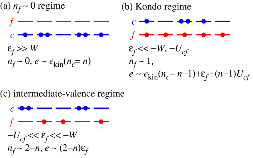
Figure 1: (Color online) Typical electron configurations in three characteristic regimes: (a) $n_{f}\simeq 0$ regime, (b) Kondo regime, and (c) intermediate-valence regime. $e_{\text{kin}}(n_{c})$ denotes the kinetic energy per site for the free conduction band with $n_{c}$.

First, we consider a case with $\epsilon_{f}\gg W$ [Fig. 1(a)], where $W$ is a typical energy scale of the conduction band or half of the bandwidth in the next section. In this case, $n_{f}\simeq 0$ and the energy $e$ per site is almost the same as the kinetic energy $e_{\text{kin}}(n_{c})$ per site of the free conduction band with $n_{c}=n$. Second, we consider a case with $\epsilon_{f}\ll-W$, $-U_{cf}$ [Fig. 1(b)]. In this case, $n_{f}\simeq 1$ and $n_{c}\simeq n-1$. The energy is approximately given by $e\simeq e_{\text{kin}}(n_{c}=n-1)+\epsilon_{f}+(n-1)U_{cf}$. We call this regime the Kondo regime. For $n_{f}\rightarrow 1$, we obtain $q\rightarrow 0$, $q_{c}\rightarrow 1$, $q_{f}\rightarrow 0$, and $a(k_{\text{F}})$ diverges as $a(k_{\text{F}})\sim q^{-1}$. By using them, we find that, for $n_{f}\rightarrow 1$, $\Delta n_{c}(k_{\text{F}})\rightarrow 0$ and $\Delta n_{f}(k_{\text{F}})\rightarrow 0$, that is, the mass enhancement factor becomes large. This mass enhancement for $n_{f}\rightarrow 1$ is consistent with the previous result for the PAM. Third, we consider a case with a moderate $\epsilon_{f}$ and a large $U_{cf}$, more explicitly, $-U_{cf}\ll\epsilon_{f}\ll-W$ [Fig. 1(c)]. In this case, $f$ and conduction electrons tend to avoid each other; thus, $n_{f}+n_{c}/2\simeq 1$ and $d\simeq 0$. That is, $n_{f}\simeq 2-n$ and $n_{c}\simeq 2n-2$. Here, we call this regime the intermediate-valence regime. In this case, both $f$ and conduction electrons are almost localized, and the energy is $e\simeq(2-n)\epsilon_{f}$. For $n_{f}+n_{c}/2\rightarrow 1$ and $d\rightarrow 0$, we obtain $q\rightarrow 0$, $q_{c}\rightarrow 0$, and $q_{f}\rightarrow 0$. By using them, we can show that the mass enhancement factor becomes large in this intermediate-valence regime. This mass enhancement in the intermediate-valence regime is not realized in the ordinary PAM and is a result of the effect of $U_{cf}$.

3 Results

Now, we show our calculated results. Here, we consider a simple model for the kinetic energy: the density of states per spin is given by $\rho(\epsilon)=1/(2W)$ for $-W\leq\epsilon\leq W$; otherwise, $\rho(\epsilon)=0$.

Figure 2(a) shows $n_{f}$ as a function of $\epsilon_{f}$ for several $U_{cf}$ values for $V/W=0.1$ and $n=1.75$.

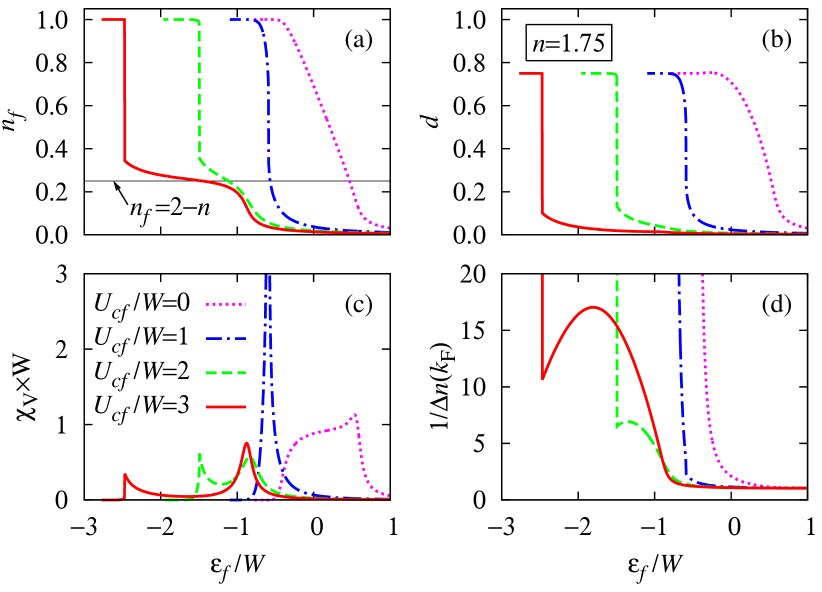
Figure 2: (Color online) $\epsilon_{f}$ dependences of (a) $n_{f}$, (b) $d$, (c) $\chi_{\text{V}}$, and (d) $1/\Delta n(k_{\text{F}})$ for $V/W=0.1$ and $n=1.75$. $U_{cf}/W=0$ (dotted lines), 1 (dash-dotted lines), 2 (dashed lines), and 3 (solid lines).

For a large $U_{cf}$, we recognize the three regimes mentioned above. A first-order phase transition occurs from the Kondo regime to the intermediate-valence regime or to the $n_{f}\simeq 0$ regime for $U_{cf}/W>0.89$. We observe hysteresis by increasing and decreasing $\epsilon_{f}$ across the first-order phase transition point, and here we show the values of the state that has the lower energy. Figure 2(b) shows the number of interacting electron pairs $d$ through $U_{cf}$ per site. For a large $U_{cf}$, the conduction and $f$ electrons tend to avoid each other and $d$ is suppressed. Figure 2(c) shows the valence susceptibility $\chi_{\text{V}}=-dn_{f}/d\epsilon_{f}$ as a function of $\epsilon_{f}$. The valence susceptibility enhances around the boundaries of three regimes for a large $U_{cf}$. For $U_{cf}=0$, such a boundary is not so clear. Figure 2(d) shows the mass enhancement factor $1/\Delta n(k_{\text{F}})$ as a function of $\epsilon_{f}$. In addition to the enhancement for $n_{f}\rightarrow 1$ as in the ordinary PAM, we find another region, that is, the intermediate-valence regime $n_{f}\simeq 2-n$, in which the mass enhancement factor becomes large. This enhancement, in particular, a peak as a function of $\epsilon_{f}$, is not expected for the PAM without $U_{cf}$. Our theory may be relevant to the large effective mass in the intermediate-valence compounds $\alpha$-YbAlB₄ and $\beta$-YbAlB₄ and the nonmonotonic variation in the effective mass under pressure in CeCu₂Si₂.

To clearly observe the effect of $U_{cf}$ on the mass enhancement, we show $1/\Delta n(k_{\text{F}})$ as a function of $n_{f}$ in Fig. 3.

Figure 3: (Color online) $1/\Delta n(k_{\text{F}})$ as a function of $n_{f}$ for $V/W=0.1$ and $n=1.75$. $U_{cf}/W=0$ (dotted lines), 1 (dash-dotted lines), 2 (dashed lines), and 3 (solid lines). The thin line is $(1-n_{f}/2)/(1-n_{f})$. The vertical line indicates $n_{f}=2-n$.

The thin line, which almost overlaps with the $U_{cf}=0$ data, represents the mass enhancement factor, given by eq. (1), i.e., $(1-n_{f}/2)/(1-n_{f})$ obtained for the PAM with $U_{cf}=0$ and $g=1$. Note that, in the present theory, $g\neq 1$ even for $U_{cf}=0$. By increasing $U_{cf}$, $1/\Delta n(k_{\text{F}})$ becomes large, particularly in the intermediate-valence regime $n_{f}\simeq 2-n$.

In Fig. 4, we show the momentum distribution functions $n_{c}(\mib{k})$ and $n_{f}(\mib{k})$ for $n=1.75$ and $n_{f}=2-n=0.25$ for several values of $U_{cf}$.

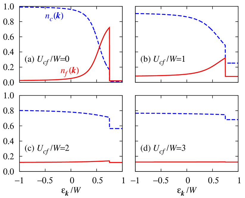
Figure 4: (Color online) Momentum distribution functions $n_{c}(\mib{k})$ (dashed lines) and $n_{f}(\mib{k})$ (solid lines) as functions of $\epsilon_{\mib{k}}$ for $V/W=0.1$, $n=1.75$, and $n_{f}=2-n=0.25$. (a) $U_{cf}/W=0$, (b) $U_{cf}/W=1$, (c) $U_{cf}/W=2$, and (d) $U_{cf}/W=3$.

For $U_{cf}=0$, the jump at the Fermi energy $\epsilon_{k_{\text{F}}}=(n-1)W=0.75W$ is much larger for $n_{f}(k_{\text{F}})$ than for $n_{c}(k_{\text{F}})$, that is, the quasiparticle weight is mainly composed of the $f$-electron contribution. For a large $U_{cf}$, the jump becomes small for both $n_{f}(k_{\text{F}})$ and $n_{c}(k_{\text{F}})$, and the mass enhancement factor becomes large, as shown in Fig. 3.

Figure 5 shows how we determine the critical point of the valence transition.

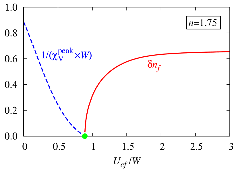
Figure 5: (Color online) Inverse of peak value $\chi^{\text{peak}}_{\text{V}}$ (dashed line) of valence susceptibility [see Fig. 2(c)] and jump $\delta n_{f}$ (solid line) in $n_{f}$ [see Fig. 2(a)] at first-order phase transition as functions of $U_{cf}$ for $V/W=0.1$ and $n=1.75$. The circle represents the critical point.

In this figure, we draw the inverse of the peak $\chi^{\text{peak}}_{\text{V}}$ of the valence susceptibility and the jump $\delta n_{f}$ in $n_{f}$ at the first-order valence transition. Both of them should become zero at the critical point, and indeed, we find that they become zero at the same $U_{cf}$.

In Fig. 6(a), we show the valence susceptibility $\chi_{\text{V}}$ as a function of $\epsilon_{f}$ and $U_{cf}$ for $n=1.75$.

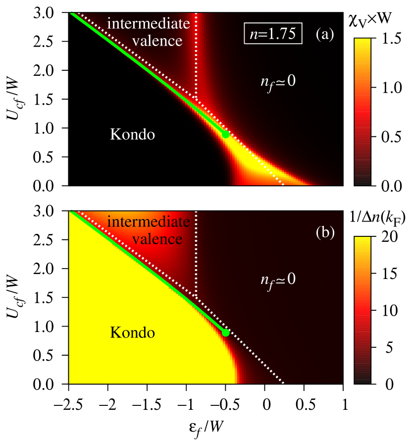
Figure 6: (Color online) (a) $\chi_{\text{V}}$ and (b) $1/\Delta n(k_{\text{F}})$ as functions of $\epsilon_{f}$ and $U_{cf}$ for $n=1.75$ with $V/W=0.1$. The solid lines represent the first-order valence transition line. The solid circles denote the critical point of the valence transition. The dotted lines indicate crossover lines determined by comparing the energies of the three extreme states (see text).

In this figure, we also draw the first-order valence transition line and its critical point. The crossover lines, represented by the dotted lines, are determined by comparing the energies of the three extreme states: $n_{f}=0$, $n_{f}=1$, and $n_{f}+n_{c}/2=1$ with $d=0$. The crossover lines are given by

$$\epsilon_{f}=-(n-1)U_{cf}+e_{\text{kin}}(n_{c}=n)-e_{\text{kin}}(n_{c}=n-1),$$ (44)

between the Kondo and $n_{f}\simeq 0$ regimes, by

$$\epsilon_{f}=\frac{e_{\text{kin}}(n_{c}=n)}{2-n},$$ (45)

between the intermediate-valence and $n_{f}\simeq 0$ regimes, and by

$$\epsilon_{f}=-U_{cf}-\frac{e_{\text{kin}}(n_{c}=n-1)}{n-1},$$ (46)

between the Kondo and intermediate-valence regimes. The crossover line between the intermediate-valence and $n_{f}\simeq 0$ regimes does not depend on $U_{cf}$. The other crossover lines are straight lines with finite slopes. Between the Kondo and $n_{f}\simeq 0$ regimes, the slope is $-1/(n-1)$ and does not depend on the band structure. Between the Kondo and intermediate-valence regimes, the slope is $-1$ independent of both the band structure and filling $n$. [7] The region where $\chi_{\text{V}}$ becomes large is captured well by the crossover lines obtained by such a simple consideration. The first-order valence transition occurs only from the Kondo to intermediate-valence or to $n_{f}\simeq 0$ regimes within the $U_{cf}$ range presented here. Note that the valence transition can occur also between the intermediate-valence regime and the $n_{f}\simeq 0$ regime for a smaller $n$. [20] Figure 6(b) shows the mass enhancement factor $1/\Delta n(k_{\text{F}})$ as a function of $\epsilon_{f}$ and $U_{cf}$. A large mass enhancement occurs in the intermediate-valence regime in addition to the Kondo regime. Here, note that the large mass enhancement occurs in the middle of the intermediate-valence regime. Thus, this enhancement is not due to valence fluctuations. In CeCu₂Si₂, the effective mass has a peak before the superconducting transition temperature becomes maximum under pressure, and which is consistent with our theory provided that the pairing interaction of superconductivity is mediated by the valence fluctuations. The situation will also be similar for CeCu₂Ge₂ if we can subtract the contributions of magnetic fluctuations.

Finally, to verify the consistency of the present theory, we check the Claudius-Clapeyron relation for the first-order valence transition. [22, 7] This relation is given by

$$\frac{\delta n_{f}}{\delta d}=-\frac{\delta U_{cf}}{\delta\epsilon_{f}},$$ (47)

where $\delta d$ denotes the jump in $d$ at the valence transition, and $\delta U_{cf}/\delta\epsilon_{f}$ is the slope of the valence transition line. In Fig. 7, we show the values of the quantities on the left and right sides of eq. (47).

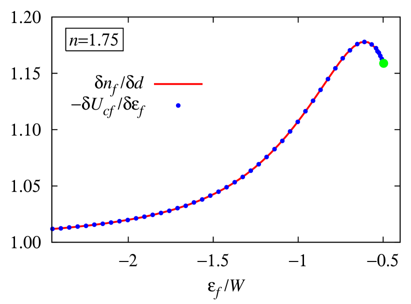
Figure 7: (Color online) Ratio $\delta n_{f}/\delta d$ (solid line) of jumps [see Figs. 2(a) and 2(b)] at the first-order phase transition and slope $-\delta U_{cf}/\delta\epsilon_{f}$ (small circles) of first-order phase transition line (see Fig. 6) for $V/W=0.1$ and $n=1.75$. The large circle indicates the critical point.

We can clearly see that the Clausius-Clapeyron relation holds in the present theory. Note that the Clausius-Clapeyron relation also holds for the crossover lines mentioned above. For example, $n_{f}\simeq 1$ and $d\simeq n-1$ for the Kondo regime and $n_{f}\simeq 0$ and $d\simeq 0$ for the $n_{f}\simeq 0$ regime, and then, between these two regimes, $\delta n_{f}/\delta d\simeq 1/(n-1)$. It is the slope $-\delta U_{cf}/\delta\epsilon_{f}$ for that crossover line given by eq. (44).

4 Summary and Discussion

We have studied the extended periodic Anderson model with $U_{cf}$ by Gutzwiller approximation. We have found that the three regimes, that is, the Kondo, intermediate-valence, and $n_{f}\simeq 0$ regimes, are clearly defined for a large $U_{cf}$. Then, we have found that, in the intermediate-valence regime, the effective mass is enhanced substantially. According to the present theory, the large mass enhancement in the intermediate-valence regime indicates a large $U_{cf}$. Thus, our theory provides helpful information for searching a superconductor with valence-fluctuation-mediated pairing.

In this study, we have not considered the possible instability toward a spin-density-wave state and a charge-density-wave state. Such a state would be realized in a portion of the parameter space, particularly, in a lattice without geometric frustration. [8, 19] The extension of the present theory to such states is a future problem. In the present theory for a uniform state, the effect of a lattice structure is included only through the density of states of the conduction band. Thus, our results may change little for a frustrated lattice with a similar density of states even if we consider the possibility of the density-wave states.

In our theory, we expand both the conduction- and $f$-electron states in the basis states in real space; thus, it will be possible to include the onsite correlation between conduction electrons and other short-range correlations. These extensions are future problems.

Appendix A Approximation for Determinants

In this appendix, we introduce approximations for determinants to evaluate expectation values in the variational wave function. Although most of them have been derived in ref. Fazekas1987, we repeat them for the readers’ convenience.

We consider the state

$$\lvert\mib{k}_{1}\cdots\mib{k}_{N}\rangle=c^{\dagger}_{\mib{k}_{1}}\cdots c^{\dagger}_{\mib{k}_{N}}\lvert 0\rangle,$$ (48)

where $c^{\dagger}_{\mib{k}_{i}}$ denotes the creation operator of a spinless fermion with the momentum $\mib{k}_{i}$. From eq. (8), we obtain

$$\begin{split}&\langle\mib{k}^{\prime}_{1}\cdots\mib{k}^{\prime}_{N}|\mib{k}_{1}\cdots\mib{k}_{N}\rangle\\ =&\sum_{\{\mib{r}\}}\det[\varphi^{*}_{\mib{k}^{\prime}}(\mib{r})]\det[\varphi_{\mib{k}}(\mib{r})]\\ =&\delta_{\mib{k}_{1}\mib{k}^{\prime}_{1}}\cdots\delta_{\mib{k}_{N}\mib{k}^{\prime}_{N}}.\end{split}$$ (49)

Then, we approximate each product of determinants by the average, that is,

$$\lvert\det[\varphi_{\mib{k}}(\mib{r})]\rvert^{2}\simeq\frac{1}{{}_{L}C_{N}},$$ (50)

and

$$\det[\varphi^{*}_{\mib{k}^{\prime}}(\mib{r})]\det[\varphi_{\mib{k}}(\mib{r})]\simeq 0,$$ (51)

for $\{\mib{k}\}\neq\{\mib{k}^{\prime}\}$.

For the kinetic energy, we need to evaluate another type of determinant. We consider

$$\begin{split}c_{\mib{r}^{\prime}}|\mib{k}_{1}\cdots\mib{k}_{N}\rangle=\sum_{\{\mib{r}\}}&\det[\varphi_{\mib{k}}(\mib{r})]c_{\mib{r}^{\prime}}|\mib{r}_{1}\cdots\mib{r}_{N}\rangle\\ =\sum_{\{\mib{r}\}\not\ni\mib{r}^{\prime}}&\det{}^{(\mib{r}^{\prime})}[\varphi_{\mib{k}}(\mib{r})]|\mib{r}_{1}\cdots\mib{r}_{N-1}\rangle,\end{split}$$ (52)

where

$$\det{}^{(\mib{r}^{\prime})}[\varphi_{\mib{k}}(\mib{r})]=\begin{vmatrix}\varphi_{\mib{k}_{1}}(\mib{r}^{\prime})&\varphi_{\mib{k}_{1}}(\mib{r}_{1})&\\ \varphi_{\mib{k}_{2}}(\mib{r}^{\prime})&\ddots&\\ &&\varphi_{\mib{k}_{N}}(\mib{r}_{N-1})\end{vmatrix}.$$ (53)

Then, for $\mib{r}^{\prime}\neq\mib{r}^{\prime\prime}$,

$$\begin{split}&\langle\mib{k}_{1}\cdots\mib{k}_{N}|c^{\dagger}_{\mib{r}^{\prime}}c_{\mib{r}^{\prime\prime}}|\mib{k}_{1}\cdots\mib{k}_{N}\rangle\\ =&\sum_{\{\mib{r}\}\not\ni\mib{r}^{\prime},\mib{r}^{\prime\prime}}\det{}^{(\mib{r}^{\prime})}[\varphi^{*}_{\mib{k}}(\mib{r})]\det{}^{(\mib{r}^{\prime\prime})}[\varphi_{\mib{k}}(\mib{r})].\end{split}$$ (54)

On the other hand, by using the expansion

$$c_{\mib{r}^{\prime}}=\sum_{\mib{k}^{\prime}}\varphi_{\mib{k}^{\prime}}(\mib{r}^{\prime})c_{\mib{k}^{\prime}},$$ (55)

we obtain

$$\begin{split}&\langle\mib{k}_{1}\cdots\mib{k}_{N}|c^{\dagger}_{\mib{r}^{\prime}}c_{\mib{r}^{\prime\prime}}|\mib{k}_{1}\cdots\mib{k}_{N}\rangle\\ =&\sum_{\mib{k}^{\prime}}\varphi^{*}_{\mib{k}^{\prime}}(\mib{r}^{\prime})\varphi_{\mib{k}^{\prime}}(\mib{r}^{\prime\prime})\langle\mib{k}_{1}\cdots\mib{k}_{N}|c^{\dagger}_{\mib{k}^{\prime}}c_{\mib{k}^{\prime}}|\mib{k}_{1}\cdots\mib{k}_{N}\rangle\\ =&\sum^{N}_{i=1}\varphi^{*}_{\mib{k}_{i}}(\mib{r}^{\prime})\varphi_{\mib{k}_{i}}(\mib{r}^{\prime\prime}).\end{split}$$ (56)

Then, we approximate the products of determinants in eq. (54) by their average:

$$\begin{split}&\det{}^{(\mib{r}^{\prime})}[\varphi^{*}_{\mib{k}}(\mib{r})]\det{}^{(\mib{r}^{\prime\prime})}[\varphi_{\mib{k}}(\mib{r})]\\ \simeq&\frac{1}{{}_{L-2}C_{N-1}}\sum^{N}_{i=1}\varphi^{*}_{\mib{k}_{i}}(\mib{r}^{\prime})\varphi_{\mib{k}_{i}}(\mib{r}^{\prime\prime}).\end{split}$$ (57)

Appendix B Evaluation of $\sum\prod a^{2}(\mib{k})$ with Restriction

In the canonical ensemble for an $N$ free-electron system with dispersion $\varepsilon_{\mib{k}}$ at temperature $1/\beta$, the hole distribution function is given by

$$\langle c_{\mib{k}}c^{\dagger}_{\mib{k}}\rangle=\sum_{\{\mib{k}^{\prime}\}\not\ni\mib{k}}e^{-\beta\sum^{N}_{i=1}\varepsilon_{\mib{k}^{\prime}_{i}}}/Z(N),$$ (58)

where $Z(N)$ is the partition function. It should be equivalent to that in the grand canonical ensemble,

$$\frac{e^{\beta(\varepsilon_{\mib{k}}-\mu)}}{1+e^{\beta(\varepsilon_{\mib{k}}-\mu)}},$$ (59)

where $\mu$ is the chemical potential, and thus,

$$\sum_{\{\mib{k}^{\prime}\}\not\ni\mib{k}}e^{-\beta\sum^{N}_{i=1}\varepsilon_{\mib{k}^{\prime}_{i}}}=\frac{e^{-\beta\mu}}{e^{-\beta\mu}+e^{-\beta\varepsilon_{\mib{k}}}}Z(N).$$ (60)

By putting $\varepsilon_{\mib{k}}=-\ln a^{2}(\mib{k})$, $\beta=1$, and $e^{\mu}=q$, we obtain

$$\sum_{\{\mib{k}^{\prime}\}\not\ni\mib{k}}\prod^{N}_{i=1}a^{2}(\mib{k}^{\prime}_{i})=\frac{q^{-1}}{q^{-1}+a^{2}(\mib{k})}Z(N).$$ (61)

References

[1]
F. Steglich, J. Aarts, C. D. Bredl, W. Lieke, D. Meschede, W. Franz, and
H. Schäfer: Phys. Rev. Lett. 43 (1979) 1892.
[2]
B. Bellarbi, A. Benoit, D. Jaccard, J. M. Mignot, and H. F. Braun: Phys. Rev. B
30 (1984) 1182.
[3]
E. Vargoz and D. Jaccard: J. Magn. Magn. Mater. 177–181 (1998)
294.
[4]
H. Q. Yuan, F. M. Grosche, M. Deppe, C. Geibel, G. Sparn, and F. Steglich:
Science 302 (2003) 2104.
[5]
K. Miyake, O. Narikiyo, and Y. Onishi: Physica B 259–261 (1999)
676.
[6]
Y. Onishi and K. Miyake: J. Phys. Soc. Jpn. 69 (2000) 3955.
[7]
S. Watanabe, M. Imada, and K. Miyake: J. Phys. Soc. Jpn. 75 (2006)
043710.
[8]
T. Sugibayashi, Y. Saiga, and D. S. Hirashima: J. Phys. Soc. Jpn. 77 (2008) 024716.
[9]
T. M. Rice and K. Ueda: Phys. Rev. B 34 (1986) 6420.
[10]
P. Fazekas and B. H. Brandow: Phys. Scr. 36 (1987) 809.
[11]
D. Jaccard, H. Wilhelm, K. Alami-Yadri, and E. Vargoz: Physica B 259–261 (1999) 1.
[12]
A. T. Holmes, D. Jaccard, and K. Miyake: Phys. Rev. B 69 (2004)
024508.
[13]
J.-P. Rueff, S. Raymond, M. Taguchi, M. Sikora, J.-P. Itié, F. Baudelet,
D. Braithwaite, G. Knebel, and D. Jaccard: Phys. Rev. Lett. 106
(2011) 186405.
[14]
R. T. Macaluso, S. Nakatsuji, K. Kuga, E. L. Thomas, Y. Machida, Y. Maeno,
Z. Fisk, and J. Y. Chan: Chem. Mater. 19 (2007) 1918.
[15]
M. Okawa, M. Matsunami, K. Ishizaka, R. Eguchi, M. Taguchi, A. Chainani,
Y. Takata, M. Yabashi, K. Tamasaku, Y. Nishino, T. Ishikawa, K. Kuga,
N. Horie, S. Nakatsuji, and S. Shin: Phys. Rev. Lett. 104 (2010)
247201.
[16]
C. E. T. Gonçalves da Silva and L. M. Falicov: Solid State Commun.
17 (1975) 1521 .
[17]
Y. Onishi and K. Miyake: Physica B 281–282 (2000) 191.
[18]
Y. Saiga, T. Sugibayashi, and D. S. Hirashima: J. Phys. Soc. Jpn. 77 (2008) 114710.
[19]
T. Yoshida, T. Ohashi, and N. Kawakami: J. Phys. Soc. Jpn. 80
(2011) 064710.
[20]
K. Kubo: J. Phys. Soc. Jpn. 80 (2011) 063706.
[21]
M. C. Gutzwiller: Phys. Rev. 137 (1965) A1726.
[22]
S. Watanabe and M. Imada: J. Phys. Soc. Jpn. 73 (2004) 3341.