Nonmonotonic dependence of the absolute entropy on temperature in supercooled Stillinger-Weber silicon

Abstract

Using a recently developed thermodynamic integration method, we compute the precise values of the excess Gibbs free energy ($G^{e}$) of the high density liquid (HDL) phase with respect to the crystalline phase at different temperatures ($T$) in the supercooled region of the Stillinger-Weber (SW) silicon [F. H. Stillinger and T. A. Weber, Phys. Rev. B. 32, 5262 (1985)]. Based on the slope of $G^{e}$ with respect to $T$, we find that the absolute entropy of the HDL phase increases as its enthalpy changes from the equilibrium value at $T\geq 1065$ K to the value corresponding to a non-equilibrium state at $1060$ K. We find that the volume distribution in the equilibrium HDL phases become progressively broader as the temperature is reduced to 1060 K, exhibiting van-der-Waals (VDW) loop in the pressure-volume curves. Our results provides insight into the thermodynamic cause of the transition from the HDL phase to the low density phases in SW silicon, observed in earlier studies near 1060 K at zero pressure.

1 Introduction

The liquid-amorphous transition in silicon, modeled by the Stillinger-Weber (SW) potential STILLINGER85 , has been intensely studied BROUGHTON87 ; LUEDTKE88 ; LUEDTKE89 ; ANGELL96 ; SASTRY03 ; BEAUCAGE05 ; VASISHT11 ; HUJO11 ; LIMMER11 with an aim of understanding the phase behavior of real silicon. In the initial molecular dynamics (MD) studies on SW silicon LUEDTKE89 ; ANGELL96 , it was found that the high density liquid (HDL) phase, at a sufficiently slow cooling rate, undergoes a sudden transition to a low density amorphous phase at around 1060 K. The nature of the low density phase (i.e., whether it is a solid or a liquid) below the transition temperature was however not clear. In 2003, Sastry and Angell, through precise and careful measurements of the diffusivity in MD simulations, showed that a low density liquid (LDL) phase exists below 1060 K and hence the transition should be characterized as a liquid–liquid transition SASTRY03 . It was also demonstrated that in constant pressure–constant enthalpy (NPH) MD simulations starting from the HDL phase at $T>1060$ K, the enthalpy shows a nonmonotonic dependence on temperature, ultimately leading to the formation of the LDL phase SASTRY03 . This was attributed to the release of latent heat during the phase transformation from the HDL phase to the LDL phase SASTRY03 . Recently, studies by Hujo et. al. HUJO11 and Limmer and Chandler LIMMER11 do not suggest the presence of a phase coexistence temperature between the HDL and the LDL phases at zero pressure.

In this work, we study equilibrium HDL phases at and above 1060 K in isothermal–isobaric (NPT) Monte Carlo (MC) simulations at zero pressure, focusing particularly on the volume (or density) distributions. We find that due to shallow free energy barriers, complete equilibration of the HDL phase cannot be achieved in some MC trajectories, leading to non-equilibrium states at 1060 K. We have used a recently developed thermodynamic integration method GROCHOLA04 ; APTE06-1 ; APTE06-2 ; APTE10 to measure precisely the excess Gibbs free energy ($G^{e}$) of the HDL phases with respect to the crystalline phases at a given temperature and pressure. These computations yield information about the entropy changes in the HDL phases as the temperature is decreased to 1060 K. Our work provides further insight into the transition from the HDL phase to the low density phases near 1060 K. In what follows, we describe the details of our computational method.

2 Equilibration of the HDL phase

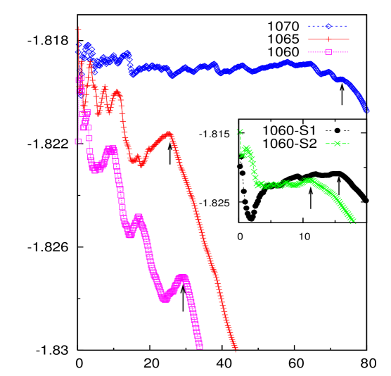
Figure 1: The MC trajectories in terms of the cumulative averaged potential energy per particle ($\phi^{\prime}=\phi/N$ expressed in units of $\epsilon$) at $T=1060$ K, $1065$ K, and $1070$ K. The points along the trajectories represent cumulative averages taken after every 0.2 million MC steps. Each MC step, on average, consisted of two volume change moves and $N$ particle displacement attempts. At 1060 K, the shorter trajectories (1060-S1 and 1060-S2) are shown in the inset, while the longer trajectory is shown in the main panel. The vertical arrows indicates the length of the trajectory used to obtain the average properties of the HDL phases. The trajectories show a systematic and continuous decrease in the average energy after the arrow positions, indicating that the free energy barrier is crossed.

To compute the excess free energy (to be described in the next section), it is important to correctly determine the average properties of the HDL phase in the supercooled region. To this end, we studied the properties of the supercooled HDL phase by performing isothermal-isobaric (NPT) Monte Carlo (MC) simulations at and above $1060$ K and zero pressure. All of our computations were performed with a system of $N=512$ particles in a cubic simulation box under periodic boundary conditions. Our main result is strongly dependent on the properties of the HDL phase in the temperature range of 1060–1070 K and hence we focus particularly on this temperature range. We find that at $T<1086$ K, the simulations starting in the HDL phase undergo a transition relatively quickly to the low density phases, indicating shallow free energy barriers. By trial and error, we find the trajectory that stays in the high density region for the largest number of MC steps at 1060, 1065 and 1070 K, by starting from different initial configurations (see Figs. 1 and  2). At 1060 K, we also found shorter trajectories (seen in the inset of Figs. 1 and  2) corresponding to non-equilibrium states. The computed average densities of the HDL phases (see Table 1) at $T>1070$ K agree reasonably well with those found in the MD cooling experiments of Beaucage and Mousseau BEAUCAGE05 .

To obtain the average properties of the HDL phases, we consider the entire length of the trajectory before it exhibits a systematic and continuous decrease in energy and density (as indicated by the arrow positions in Figs. 1 and 2), which signals the crossing of the free energy barrier. One noticeable feature is that these trajectories do not seem to have converged to the mean values (at the arrow positions), unlike the metastable states which are normally encountered. This may be due to the fact that the probability distribution with respect to the volume and energy is broad and highly asymmetric for the HDL phases. At 1065 K and 1070 K, we find that shorter trajectories (not shown) generated independently (with lengths of 10.4 and 35.2 million MC steps, respectively) acquire average energies and densities (just before crossing the free energy barrier), which are nearly equal to the values reported here for the longer trajectories. For this reason, it is important to consider the entire length of the trajectories upto the arrow positions to compute the average properties. If one considers smaller portions of the trajectories, the resulting average properties will not reflect the correct sampling of the free energy surface.

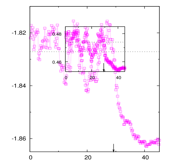
Figure 3: The long trajectory at 1060 K (also shown in Figs. 1 and  2) in terms of instantaneous block averages taken after every 0.2 million MC steps. The main panel shows average potential energy per particle while the inset shows the average density. The arrow positions (the same as those in earlier figures) indicate the location along the trajectory at which the free energy barrier is crossed. The horizontal dashed lines shows the cumulative averaged quantities (see earlier figures and also Table 1) at the arrow positions. As can be seen in the figure, high energy and high density states are accessible even towards the end of the HDL portion of the trajectory (close to the arrow positions).

At 1060 K, we find that the average properties of the shorter trajectories (denoted as 1060-S1 and 1060-S2) and the longer trajectory (see Table 1) differ considerably. Due to its shallowness, the free energy barrier is crossed even before the equilibration is achieved, leading to the non-equilibrated shorter trajectories. In case of the longer trajectory at 1060 K (see Figs. 1 and 2), the cumulative averages show an overall drift to lower densities and energies and therefore it may appear that the high energy (and high density) states become inaccessible as the trajectory progresses. However it is clear from the instantaneous block averages along the trajectory in Fig. 3, that the higher energy (and higher density) states remain accessible even towards the end of the HDL portion of the trajectory. The same is the case with the trajectories at 1065 and 1070 K. In a latter section, our analysis based on Gibbs Helmholtz equation indicates that trajectories at 1065 and 1070 K, as well as the longer trajectory at 1060 K represent equilibrium phases.

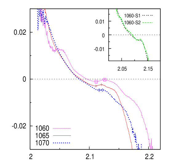
Figure 4: Average virial pressure ($p$, in units of $\epsilon/\sigma^{3}$) as a function of volume per particle ($v=1/\rho$) for the HDL phase. The inset shows the p-v curve for the shorter trajectories at 1060 K. At each temperature, the portion of the curve between the two displayed points has a zero or a positive slope indicating a two-phase region. The irregular shape of the curves at the two ends is a result of the poor statistical sampling in those regions (see Fig. 5).

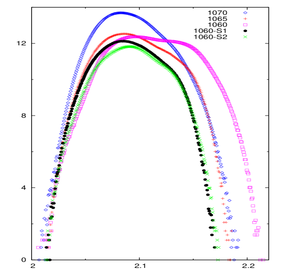
Figure 5: The Helmholtz free energy (in units of $k_{B}T$) within a constant as a function of volume for the HDL phases at 1060, 1065, and 1070 K. As explained in the text, the ordinate is $\log N_{c}=-\beta F+$ constant, where $N_{c}$ is the number of configurations generated in MC simulations with a specific volume between $v$ and $v+\Delta v$.

Next we analyze the pressure (p)–volume (v) curves (Fig. 4) and the Helmholtz free energy of the HDL phases as a function of volume (Fig. 5) from the data generated by the above HDL trajectories. Here $v=V/N$ is the volume per particle (in units of $\sigma^{3}$) and $p$ is the average virial pressure (in units of $\epsilon/\sigma^{3}$) obtained from fluctuations that correspond to a bin of width $\Delta v=6.24\times 10^{-4}\sigma^{3}$ taken at $v$. (The quantities reported throughout this work are expressed in units of SW potential parameters STILLINGER85 $\sigma$ and $\epsilon$, unless otherwise noted explicitly). We obtain the Helmholtz free energy at a given v by using the fact that in isothermal–isobaric ensemble at zero pressure, the probability density of finding the system with a specific volume v is $\exp[-\beta F(V)]$. Hence if $N_{c}$ is the number of configurations generated in MC simulations with a specific volume between $v$ and $v+\Delta v$, then $N_{c}\propto\exp[-\beta F(V)]\Delta v$ and hence $\log N_{c}=-\beta F+$ constant. This is the quantity we have plotted verses v in Fig. 5 and also in the subsequent figures.

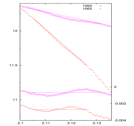
Figure 6: The double tangent construction at 1060 K and 1065 K. The upper curves are portions of the full F-v curves in Fig. 5 and represent the value of Helmholtz free energy per unit $k_{B}T$ within a constant. The lower curves are portion of the p-v curves in Fig. 4 and represent the average virial pressure as a function of volume per particle. The lines in the upper curves are the double tangent lines CALLEN85 with a slope equal to $\beta p$, where $p$ is the pressure value at the two ends of the VDW loops in the lower curves.

At 1070 K, we observe a region with an approximately zero slope in the p-v curve as indicated by the two highlighted points along the curve in Fig. 4, indicating the presence of a two-phase region. At 1060 and 1065 K, we observe a region in the p-v curve with a positive slope. At 1060 K and 1065 K, we are able to construct double tangent lines corresponding to the Van-der-Waals (VDW) loops as seen in Fig. 6. The two ends of the tangent line represents two states with the same chemical potential at the same temperature and pressure and hence the relation $\Delta U+p\Delta V=T\Delta S$ is valid CALLEN85 , where $\Delta$ represents the difference of the properties of the two states across the tangent line. In the present case, the values of $p$ in the above equation are $-0.65\times 10^{-3}$ and $-0.27\times 10^{-2}$ at 1060 K (long trajectory) and 1065 K, respectively. Both the terms $\Delta U$ and $p\Delta V$ have the same sign indicating a non-zero enthalpy difference between states joined by the double-tangent lines (see Fig. 6).

At 1065 K, we find that F-v curve is not symmetric about the maximum even for small deviations away from the maximum. Instead we find that the distribution can be described fairly accurately by a Taylor series expansion around the spinodal according to the following equation.

$$F(T,V,N)=F_{s}-p_{s}(V-V_{s})+\frac{1}{3!}F_{s}^{\prime\prime\prime}(V-V_{s})^{3},$$ (1)

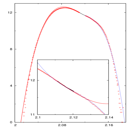
Figure 7: The red and blue lines denotes the Taylor series expansion to third order around the left and right spinodals according to Eq. (1) at 1065 K. The lines are truncated at the respective spinodals. The solid black line corresponds to the region of the curve between the two spinodals. The inset shows that the Taylor series expansion (red and blue lines) deviate from the actual curve rapidly if continued beyond the spinodals.

Here $V_{s}$ corresponds to the volume at the spinodal. The second order term is taken as zero, since by definition, the second derivative is zero at the spinodal. Taking derivatives by finite difference always involves much noise and therefore it is not possible to reliably compute $F_{s}^{\prime\prime\prime}$ directly by numerical differentiation. We used the actual value of $p_{s}$ (average virial pressure) as measured in simulation at the spinodal density (see Fig. 6), while we fitted the value of $F_{s}^{\prime\prime\prime}$ by trial and error so as to best fit the data. The resultant curve agrees well with the actual value of $F$ as seen in Fig. 7. We considered $p_{s}=-2.935\times 10^{-3}$ and $F_{s}^{\prime\prime\prime}=-2.872\times 10^{-5}$ for the left spinodal at $v_{s}=2.1111$ and $p_{s}=-2.352\times 10^{-3}$ and $F_{s}^{\prime\prime\prime}=5.961\times 10^{-5}$ for the right spinodal at $v_{s}=2.1205$. This suggests that the probability distribution with respect to $V$, is controlled by the spinodals at the two ends of the unstable region.

Also, we find that the expansion on either side of the unstable region is accurate only upto the spinodal and deviates rapidly from the actual curve on the other side of the spinodal as shown in the inset of Fig. 7. This implies a discontinuity in the equation of state at the two spinodals, which is expected because the two ends of the VDW loop usually correspond to the two separate phases each having its own equation of state and that each phase extends right upto the spinodal on either side of the VDW loop. It is to be noted that the HDL phase configurations consists of atoms connected to form tetrahedra BEAUCAGE05 . The different tetrahedra are connected through common atoms forming a network and the number of these tetrahedral structures can fluctuate causing overall variations in the potential energy and the density. The above Taylor series expansion around the spinodals may be attributed to the network forming tendency of the liquid. This needs to be investigated further.

We observe that the following fluctuation relation LANDAU-5 is satisfied by the MC trajectories:

$$\langle(\Delta p)(\Delta V)\rangle=-k_{B}T,$$ (2)

when we consider $\Delta p=(p_{in}-\langle p_{in}\rangle)$ and $\Delta V=(V-\langle V\rangle)$, where $p_{in}$ is the instantaneous pressure in the NPT-MC simulations calculated from the virial relation ALLEN87 at the given instantaneous volume $V$ and $T$ is the externally set temperature. The symbol $\langle\cdots\rangle$ represents the average taken over the entire trajectory of the isothermal isobaric MC simulations. This fluctuation relation is derived by assuming LANDAU-5 that the instantaneous fluctuations represents a change in state from one homogeneous phase to the other. The relation is satisfied by the entire trajectory consisting of the HDL, LDL and the defect crystal regions, as well as by the partial trajectories consisting only of the HDL phase region. This possibly indicates that transition from the HDL phase to the LDL or the d-crystal phases along the trajectory involves entirely homogeneous states. We also find that the total average virial pressure is zero at all points along the MC trajectories meaning that the system is in mechanical equilibrium throughout.

3 Computation of excess Gibbs free energy

We computed the excess Gibbs free energy difference $G^{e}=G_{\mbox{\small HDL}}-G_{\mbox{\small crystal}}$ between the HDL and the crystal phases, by applying the constrained fluid $\lambda$ integration method GROCHOLA04 in the isothermal–isobaric ensemble APTE06-1 ; APTE06-2 ; APTE05 . Recently, the method was found to predict the melting point of SW silicon accurately APTE10 . This is a thermodynamic integration method in which the liquid and the crystal phase are connected directly through a 3-stage reversible path. In stage 1 of the reversible path, which starts from the liquid phase, the strength of the interaction potential is reduced linearly so that the system approaches an ideal gas-like behavior. The expression for the potential energy in this stage is given by GROCHOLA04 ; APTE06-1 ,

$$\phi_{1}(\lambda_{1})=(1-\eta\lambda_{1})\phi,$$ (3)

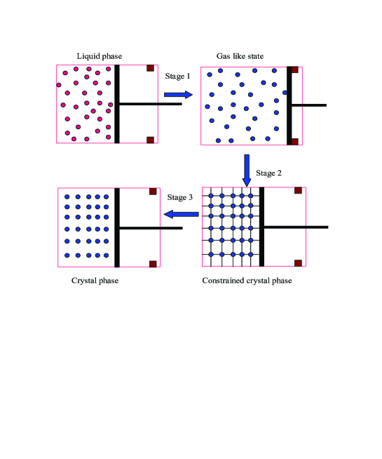
Figure 8: Schematic diagram of the thermodynamic integration path connecting the liquid and the solid states at constant temperature and constant external pressure. GROCHOLA04 ; APTE06-1 The stops in the piston-cylinder arrangement represent the maximum volume constraint as described in the text.

where $\eta$ is a constant that determines the effective strength of the interaction potential at the end of stage 1 and $\phi$ is the original inter-particle potential (SW potential, in the present case). The parameter $\lambda_{1}$ defines the states along the path and varies from 0 to 1. As the system becomes less attractive it tends to expand. However, to maintain the reversibility of the path in stages 2 and 3, it is necessary to impose a maximum volume constraint APTE06-1 . The maximum constrained volume $V_{m}$ is chosen such that it is slightly larger than the average volumes of the liquid and the solid phase (whichever is larger). At the same time, $V_{m}$ should not affect the free energies of either of these phases APTE06-1 . Such a volume can be straightforwardly chosen based on the histogram of volume fluctuations for the two phases. As in an earlier work on SW silicon APTE10 , we chose $V_{m}$ to correspond to a density of $0.4\sigma^{-3}$, i.e., $V_{m}=N/0.4$. At the end of stage 1, we get a compressed gas phase due to the constraint on the maximum volume APTE06-1 . This process is depicted pictorially in Fig. 8.

In stage 2, we force the particles to form a crystalline structure by imposing an external potential in the form of Gaussian potential wells distributed on the ideal crystal lattice GROCHOLA04 . The strength of the inter-particle potential energy is held fixed during this stage. The total potential energy for stage 2 is given by GROCHOLA04 ; APTE06-1

$$\phi_{2}(\lambda_{2})=(1-\eta)\phi+\lambda_{2}U_{ext}.$$ (4)

The Gaussian external potential imposed during this and the subsequent stage is given by $U_{ext}=\sum_{i}\sum_{k}a\exp(-br_{ik}^{2})$ GROCHOLA04 . Here, the index ‘i’ refers to the system particle and the index ‘k’ is a Gaussian potential well. The Gaussian well does not act on a specific particle, but exerts an influence over all the particles in its vicinity. GROCHOLA04 ; APTE06-1 The values of the Gaussian parameters are taken to be the same as in the earlier work APTE10 : $\eta=0.9$, $a=-1.892\epsilon$ and $b=8.0\sigma$. These values are so chosen that the constrained crystalline state obtained at the end of stage 2 has almost the same energy and density as the desired crystal phase APTE05 ; APTE06-1 .

In stage 3, the Gaussian external potential is reduced linearly to zero, while the strength of the potential energy is increased linearly to its original value GROCHOLA04 . The potential energy expression for this stage is given by GROCHOLA04

$$\phi_{3}(\lambda_{3})=[(1-\eta)+\lambda_{3}\eta]\phi+(1-\lambda_{3})U_{ext}.$$ (5)

At the end of this stage, we get the desired crystalline phase as shown pictorially in Fig. 8.

The Gibbs free energy change for the i${}^{\mbox{th}}$ stage of the path can be obtained by numerical integration:

$$\Delta G_{i}=\int_{0}^{1}d\lambda_{i}\left(\frac{\partial G}{\partial\lambda_{i}}\right)=\int_{0}^{1}d\lambda_{i}\left\langle\frac{\partial\phi_{i}}{\partial\lambda_{i}}\right\rangle,$$ (6)

where $\langle\cdots\rangle$ represents the isothermal–isobaric ensemble average at a given value of $\lambda_{i}$. The integrands for the various stages of the path at $1065$ K and zero pressure are plotted in Figs. 9–11. It can be seen from these figures that the value of the integrand for the forward and the reverse paths agree well. This shows that there is no hysteresis present along the path, as found earlier APTE10 .

Throughout this work, we have used the Bennett Acceptance Ratio (BAR) method BENNETT76 , to compute the Gibbs free energy between the adjacent states along the entire path. According to the BAR method BENNETT76 , the Gibbs free energy difference $\Delta G=G_{1}-G_{0}$ between two equilibrium states ‘0’ and ‘1’, for a given value of the constant $C$, is given by the following equation BENNETT76 :

$$\frac{\Delta G}{k_{B}T}=\log\frac{\sum_{1}f(\beta\phi_{0}-\beta\phi_{1}+C)}{\sum_{0}f(\beta\phi_{1}-\beta\phi_{0}-C)}+C-\log\frac{n_{1}}{n_{0}},$$ (7)

where $f(x)=1/(1+e^{x})$ is the Fermi function, $\sum_{0}$ and $\sum_{1}$ represent the sums over Fermi functions sampled in ‘0’ and ‘1’ ensembles, respectively. The total potential energies in the two ensembles are represented by $\phi_{0}$ and $\phi_{1}$ in Eq. (7) and the total number of samples of the perturbation energies (or equivalently the Fermi functions) collected in MC simulations in the two ensembles are $n_{0}$ and $n_{1}$. In principle, the above equation yields the correct value of $\Delta G$ for any value of the constant $C$. In practice, due to the limited computational power, we cannot sample the perturbation energies in the two ensembles over all possible configurations. Thus, Bennett showed that the optimum value of $C$, which yields minimum error in the estimation of $\Delta G$, is given by BENNETT76

$$\frac{\Delta G}{k_{B}T}=C-\log\frac{n_{1}}{n_{0}}.$$ (8)

Combining the above two equations, we get BENNETT76

$${\sum_{1}f(\beta\phi_{0}-\beta\phi_{1}+C)}={\sum_{0}f(\beta\phi_{1}-\beta\phi_{0}-C)}.$$ (9)

The value of the $C$ satisfying the above equation is substituted in Eq. (8) to yield the optimal estimate of $\Delta G$. As mentioned in Ref. BENNETT76 , the accuracy of the above method depends on the degree of overlap in the configuration space between the two ensembles. The larger the value of the two sums appearing in Eq. (9), the greater is the configuration space overlap. As prescribed by Bennett, the sum values should be much greater than unity BENNETT76 .

In all our computations, we ensured that the sum values are of the order of $10^{5}$–$10^{6}$, by (i) performing simulations at $\lambda_{i}$ values that are sufficiently close to each other (see Figs. 9–11) and (ii) performing sufficiently long simulation runs at each of the $\lambda_{i}$ values. The perturbation energies [$(\phi_{1}-\phi_{0})$ or $(\phi_{0}-\phi_{1})$ in Eq. (9)] required in the BAR method were collected after every MC step. At $\lambda_{1}=0.0$ in stage 1, we used the properly equilibrated trajectories of the HDL phases, as described in the Sec. II, to collect the perturbation energy data. In stage 1, we performed upto $20$ million MC steps from $\lambda_{1}=0$ to $0.4$. In the region from $\lambda_{1}=0.4$ (stage 1) to $\lambda_{3}=0.99$ (stage 3), we performed $0.4$–$0.8$ million MC steps. The main source of statistical error was found to be towards the end of stage 3 due to the center of mass motion of the crystal phase as explained in detail in Ref. APTE10 . To address this problem, we performed up to $10$ million MC steps from $\lambda_{3}=0.992$ to $\lambda_{3}=0.999$ to collect the perturbation energy data. In the last interval of stage 3 from $\lambda_{3}=0.999$ to $1$, there is a large change in the integrand (due to center of mass motion of the crystalline phase) as seen in the inset of Fig. 11. In order to minimize the statistical error, upto $30$ million MC steps were performed at $\lambda_{3}=1$. We ensured that the value of the sums $\sum_{0}$ and $\sum_{1}$ [see Eq. (9)] over the Fermi function is above $10^{5}$ for all the intervals towards the end of stage 3. Further, in order to improve the accuracy three to four independent simulation runs were performed along the entire path at all the temperatures. The statistical error for the $i$th stage was computed by using the formula $\sigma_{i}=\sigma(\Delta G_{i})/n_{i}^{1/2}$, where $\sigma(\Delta G_{i})$ is the standard deviation in the $\Delta G_{i}$ value and $n_{i}$ is the number of statistically independent measurements. The total statistical error was computed by adding the errors for the individual stages.

Table 1 lists the values of the excess Gibbs free energy $G^{e}$ computed at various temperatures in the supercooled region at and above 1060 K at zero pressure. The $G^{e}$ values are comparable to those calculated by Broughton and Li BROUGHTON87 ($\sim 25.3\epsilon$ for N = 512 at 1060 K obtained by linear interpolation of the chemical potential data in Table III of Ref. BROUGHTON87 ). Using the Gibbs Helmholtz equation for the HDL and the crystalline phases, we get the following relation between the excess quantities at different temperatures:

$$\frac{G_{i+1}^{e}}{T_{i+1}}-\frac{G_{i}^{e}}{T_{i}}=-\int_{i}^{i+1}dT~{}~{}\left(\frac{H^{e}}{T^{2}}\right).$$ (10)

Here the quantities with a superscript ‘e’ denote excess quantities. This equation can be derived by combining the Legendre transformation (LT) relation CALLEN85 $G=H-TS$ and the following expression for the entropy,

$$S=-\left(\frac{\partial G}{\partial T}\right)_{P},$$ (11)

for the HDL and the crystalline phases. The LT relation and Eq. (11) are certainly valid for the crystalline phase, since it is the stable equilibrium phase. Therefore, the validity of Eq. (10) implies that both the LT relation and Eq. (11) are applicable for the HDL phase as well. In such a case, it is reasonable to expect that the HDL phase is an equilibrium phase, since its average enthalpy and average entropy are determined uniquely by specifying T, P, and N [according to the LT relation and Eq. (11)].

In order to check the validity of Eq. (10), we have listed the excess enthalpy $H^{e}$ values in the last column of Table 1. For a given temperature interval ($T_{i},T_{i+1}$), the right hand side of Eq. (10) can be evaluated numerically by following the trapezoidal rule. We find that this equation is satisfied for all the temperature intervals by our data, except for the data involving the two shorter trajectories at 1060 K: at $T_{i+1}=1060$ K, the value predicted by Eq. (10) is $G_{i+1}^{e}=26.01\pm 0.024$ for the shorter trajectory (1060-S1), when we substitute $G_{i}^{e}=25.862\pm 0.024$ obtained by TDI method at $T_{i}=1065$ K in Eq. (10). As we can see the value predicted by Eq. (10) does not agree within error-bars with that obtained by the TDI method ($26.073\pm 0.024$) for the shorter trajectory at 1060 K (1060-S1). Same is the case for the other shorter trajectory 1060-S2. From this analysis, it is reasonable to conclude that the HDL phase properties listed in Table 1 correspond to the equilibrium phases, except for the shorter trajectory averages (1060-S1 and 1060-S2). These shorter trajectories correspond to non-equilibrium states at 1060 K and the LT relation is not applicable to such states.

4 Changes in excess and absolute entropies of the HDL phases

In order to compute the excess entropy of the equilibrium HDL phases, we use the LT relation to obtain $S^{e}=(H^{e}-G^{e})/T$ (see third column of Table 1). The error in the value of $S^{e}$, thus computed, is due to the error in the estimation of $G^{e}$. For the HDL phases generated by the shorter trajectories at 1060 K, the LT relation is not applicable as discussed above. To compute excess entropy for these non-equilibrium HDL states, we follow the thermodynamic analysis by Nishioka NISHIOKA87-1 . In a non-equilibrium state, additional parameters ($X_{i};i=1,\cdots,r$) may be needed to specify the state of the system at given values of $T$, $P$, and $N$. The first order term for the change in the Gibbs free energy $G$ as one goes from an equilibrium to a non-equilibrium state at constant pressure is given by

$$\delta G=\left(\frac{\partial G}{\partial T}\right)_{P,X_{i}}\delta T+\sum_{i=1}^{r}\left(\frac{\partial G}{\partial X_{i}}\right)_{T,P,X_{j\neq i}}\delta X_{i}$$ (12)

Since the initial state is an equilibrium state,

$$\left(\frac{\partial G}{\partial X_{i}}\right)_{T,P,X_{j\neq i}}=0,$$ (13)

for $i=1,\cdots,r$. Applying the analysis by Nishioka NISHIOKA87-1 for the changes between equilibrium states, Eq. (11) can be expressed as follows.

$$-S = \lim_{dT\to 0}\left[\frac{G(T+dT,P,X_{i}^{eq}+dX_{i}^{eq})-G(T,P,X_{i}^{eq})}{dT}\right]$$

$$= \lim_{dT\to 0}\frac{1}{dT}\left[\left(\frac{\partial G}{\partial T}\right)_{P,X_{i}}dT+\sum_{i=1}^{r}\left(\frac{\partial G}{\partial X_{i}}\right)_{T,P,X_{j\neq i}}dX_{i}^{eq}+~{}\cdots~{}\right]$$

$$= \left(\frac{\partial G}{\partial T}\right)_{P,X_{i}},$$

where we used Eq. (13) to arrive at the last equality. The quantities $X_{i}^{eq}$ and $X_{i}^{eq}+dX_{i}^{eq}$ ($i=1,\cdots,r$) in the above equation correspond to the initial and the final equilibrium states, respectively. Substituting Eqs. (13) and (14) in Eq. (12), we have

$$\delta G=-S~{}~{}\delta T.$$ (15)

This equation yields the change in the Gibbs free energy (to the first order) due to the infinitesimally small variations $\delta T$ and $\delta X_{i}$ associated with a change from the initial equilibrium state to a final non-equilibrium state at constant pressure. For a small but finite variation from the the initial equilibrium state at $T_{i}=1065$ K to a non-equilibrium HDL state at $T_{i+1}=1060$ K at zero pressure, $S^{e}$ can then be approximated [based on Eq. (15)] as follows:

$$S^{e}\approx-~{}\frac{G^{e}_{i+1}-G^{e}_{i}}{T_{i+1}-T_{i}}.$$ (16)

Equation (16) yields the average slope (i.e. average value of $S^{e}$) in the temperature interval ($T_{i}$, $T_{i+1}$). This approximation becomes more accurate as $T_{i+1}\rightarrow T_{i}$. The values of $S^{e}$ computed by the above equation (for $N=512$) are reported in the first and second rows of Table 1 for the trajectories 1060-S1 and 1060-S2, respectively. From Table 1, we find that the average value of $S^{e}$ in the interval (1060 K,1065 K) is higher by about $68k_{B}$ (after considering the error bars) for 1060-S1 compared to the corresponding value ($\approx 751k_{B}$) in the interval (1065 K, 1070 K). Thus, as the temperature is decreased by $\Delta T=-5$ K from 1067.5 to 1062.5 K (the mid-points of above two intervals) the change in the excess entropy is $\Delta S^{e}\geq 68~{}k_{B}$.

To estimate the change in entropy of the crystalline phase, we evaluated its constant volume heat capacity at $1060$ K by using the following relation LEBOWITZ67

$$\frac{C_{V}}{Nk_{B}}=\frac{3}{2}+\frac{\langle(\delta\phi)^{2}\rangle}{N(k_{B}T)^{2}},$$ (17)

where the quantity $\delta\phi=\phi-\langle\phi\rangle$ is the instantaneous fluctuation in the total potential energy of the system. The average over the potential energy fluctuations was computed in the constant volume–constant temperature (NVT) MC simulations of the crystal phase and substituting this value in the above equation yields $C_{V}=3.7Nk_{B}$ at $1060$ K. We neglect the difference between the heat capacities of the crystal phase at constant pressure and at constant volume, i.e., $C_{P}\approx C_{V}=3.7Nk_{B}$. Then the change in absolute entropy of the crystal phase can be estimated by the following formula,

$$\Delta S\approx{C_{P}}\log\left(\frac{T+\Delta T}{T}\right),$$ (18)

where we assume $C_{P}$ to be constant over the temperature range of $\Delta T$. Using the above equation, we find that the change in the entropy $\Delta S_{\mbox{\small crystal}}$ of the crystal phase is approximately $-9k_{B}$ (for $N=512$) when the temperature is reduced from 1067.5 K to 1062.5 K ($\Delta T=-5$ K). Since $\Delta S^{e}=\Delta S_{\mbox{\small HDL}}-\Delta S_{\mbox{\small crystal}}$, we find that $\Delta S_{\mbox{\small HDL}}\geq 59~{}k_{B}$ for the change in temperature $\Delta T=-5$ K from 1067.5 K to 1062.5 K, when we consider the trajectory 1060-S1. It is to be noted that the average energy of 1060-S1 ($\langle E\rangle=-899.93~{}\epsilon$ for $N=512$) is slightly higher as compared to that of the equilibrium HDL phase ($\langle E\rangle=-900.13~{}\epsilon$) at 1065 K (the average energy can be obtained by adding the kinetic energy contribution to the average potential energy listed in the fifth column of Table 1). This also qualitatively indicates that the average entropy of the HDL corresponding to the 1060-S1 trajectory would be higher as compared to the equilibrium phase at 1065 K. For the other trajectory 1060-S2, we have $\Delta S_{\mbox{\small HDL}}\geq 49~{}k_{B}$ for the temperature change $\Delta T=-5$ K from 1067.5 K to 1062.5 K. Thus our data indicates that the HDL phase shows an increase in the entropy with decrease in temperature, when we consider the non-equilibrium states (1060-S1 and 1060-S2) at 1060 K. For the equilibrium phases, the entropy-temperature relation is monotonic, as expected (see third column of Table 1).

5 Summary and Conclusions

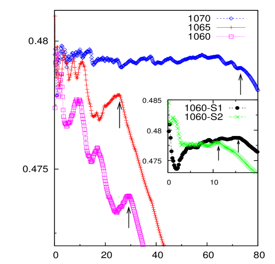
Figure 2: The same as in Fig. 1, but for the cumulative average density (expressed in units of $\sigma^{-3}$).

In this work, we generated NPT MC trajectories corresponding to the equilibrium HDL phases in the temperature range of $1060$–1070 K (Figs. 1–3). We find that as the temperature is lowered, the volume distribution becomes progressively broader and asymmetric (Fig. 5), exhibiting VDW loops in the p-v curves (Fig. 4 and  6). The fluctuations in the HDL phases can access the low density regions to a greater degree across the VDW loop, upon lowering the temperature and consequently, the average density and average energy reduces rapidly. We were able to construct the double tangent lines (Fig. 7) across the states forming the VDW loops at 1060 and 1065 K. This implies that the relation $\Delta U+p\Delta V=T\Delta S$ holds true between these states with $p$ being a negative pressure (Here both the terms $\Delta U$ and $p\Delta V$ have the same sign, implying a non-zero enthalpy difference). We found that at 1065 K, the entire F-v curve (Fig. 7) could be described by a Taylor series expansion around the spinodals [Eq. (1)].

We computed precisely the excess Gibbs free energy $G^{e}$ of the HDL phase at different temperatures by using a recently developed thermodynamic integration method APTE06-1 ; GROCHOLA04 . Based on the validity of Eq. (10) by our data, we found that the HDL phase trajectories correspond to the equilibrium phases, except for the shorter trajectories at 1060 K (1060-S1 and 1060-S2). We then computed the excess entropy of the equilibrium HDL phases from the relation : $S^{e}=(H^{e}-G^{e})/T$. For the non-equilibrium HDL phases at 1060 K, we computed $S^{e}$ from the slope of $G^{e}$ with respect to $T$ [Eq. (16)]. Based on these computations, we conclude that the absolute entropy of the HDL phase increases as its enthalpy changes from the equilibrium value at $T\geq 1065$ K to the value corresponding to the non-equilibrium states at $1060$ K. Our conclusion is supported qualitatively by the fact that the average energy of the HDL phase (1060-S1) at 1060 K is slightly higher as compared to that of HDL phase at 1065 K (see Table 1).

In the previous MD studies LUEDTKE89 ; ANGELL96 ; BEAUCAGE05 it was observed that the HDL phase, at a sufficiently slow cooling rate, transforms into a low density amorphous phase at or below $1060$ K. (Here by amorphous phase, we do not necessarily mean the LDL phase SASTRY03 , but any intermediate phase between the HDL and the LDL phases). The trajectories we generated indicate that the free energy barrier becomes very shallow at or below $1060$ K, and hence upon cooling from the high temperature phases ($T\geq 1065$ K), it is difficult to achieve the equilibration of the HDL phases. On the other hand, our computations indicate that the non-equilibrium HDL phases (at $T<1065$ K) one encounters, possess a higher entropy compared to high temperature equilibrium phases. Since the process of cooling at zero pressure necessarily involves reduction of the entropy, the HDL phase at $T\geq 1065$ K will not transform into a higher entropy HDL phase at $T<1065$ K. These are the likely reasons which trigger the transformation of the HDL phase into low density phases near 1060 K upon cooling, as observed in NPT–MD simulations LUEDTKE89 ; ANGELL96 ; BEAUCAGE05 ; HUJO11 . It is generally supposed that such transformations are caused due to a coexistence temperature between the HDL and the low density phases located near 1060 K at zero pressure. However, recent studies by Hujo et. al. HUJO11 and Limmer and Chandler LIMMER11 do not support this viewpoint. The volume distributions in the equilibrium HDL phases at 1060 K and 1065 K shows low density and high density states (joined by double tangents in Fig. 6) having the same chemical potential at a non-zero (negative) pressure. Weather such a condition (i.e., equality of chemical potentials between the high density and the low density states) is also attainable at zero pressure is an interesting question and this needs to be investigated further.

In the case of NPH MD simulations SASTRY03 , the nonmonotonic enthalpy–temperature loop starts at a temperature just above $1060$ K. Normally, the NPH simulations should trace the equilibrium (monotonic) enthalpy-temperature curve. However, it seems difficult to achieve equilibration of the HDL phases in NPH simulations for the following reasons. We note that in a statistical mechanical treatment, the properties of a macroscopic system are not taken as strictly constant, but are allowed to fluctuate dCHANDLER87 . This is specially necessary in the case of HDL phases near 1060 K, which show broad and asymmetric volume distributions indicating the importance of fluctuations. In the NPH simulations, on the other hand, the enthalpy is strictly constant which suppresses relevant fluctuations of enthalpy. For example, the two states joined by the double tangents in Fig. 6 have a non-zero enthalpy difference and both of which contribute significantly to the average properties. The NPH simulations cannot access both the states simultaneously, preventing equilibration of the HDL phases. This is the probable reason why the NPH simulations could not access the monotonic enthalpy–temperature curve corresponding to the equilibrium HDL phases at or just above 1060 K SASTRY03 .

The focus of our entire work is an extremely narrow temperature range 1060-1070 K, though we have also computed HDL phase properties and excess Gibbs free energies at higher temperature (see Table 1). We found it difficult to obtain trajectory corresponding to an equilibrium HDL phase below 1060 K. Nonetheless, our work indicates unexpected but important changes in the properties of the HDL phase that are consistent with the phase transitions observed in earlier studies at or near 1060 K. This, along with the fact that small temperature variations (as low as 0.1 K) are known to induce significant changes in the properties of other materials BUCHANAN12 , justifies our focus on the narrow temperature range.

It is desirable to perform free energy computations for the HDL phases with different number of particles to study system size effects. However due to the large extent of computations needed to obtain $G^{e}$ with a sufficient precision, it is beyond the scope of the present work. It may be noted that the density plots from MD cooling experiment with 512 VASISHT11 , 1000 BEAUCAGE05 and 4096 HUJO11 particles are qualitatively similar and show the phase transitions near 1060 K. Recent first principles MD simulations of supercooled silicon GANESH09 have demonstrated the presence of the VDW loops separating the high density and low density liquids. Thus it is possible that real silicon exhibits phase transition which is qualitatively similar to that of the SW silicon.

Table 1: The excess Gibbs free energy of the HDL phase with respect to the crystalline phase is listed at various temperatures for N = 512 and zero pressure. The excess entropy listed in the third column is computed from the relation $S^{e}=(H^{e}-G^{e})/T$ for the equilibrium phases. The reported error in the $S^{e}$ value is due to the error in $G^{e}$ value. For the non-equilibrium states (1060-S1 and 1060-S2), $S^{e}$ is calculated by using Eq. (16). The fourth and the fifth columns contain the average densities and average potential energy per particle of the HDL phases. The excess enthalpy of the HDL phases is listed in the last column of the table. The listed values of $H^{e}$, $S^{e}$, and $G^{e}$ correspond to N=512.

$T$(K)	$G^{e}$ ($\epsilon)$	$S^{e}/k_{B}$	$\langle\rho\rangle$ ($\sigma^{-3}$)	$\langle\phi^{\prime}\rangle$ ($\epsilon$)	$H^{e}$ ($\epsilon$)
	$N=512$	$N=512$			$N=512$
$1060-\mbox{S1}$	$26.073\pm 0.024$	$1060\pm 241$	0.479	-1.8209	$57.753$
$1060-\mbox{S2}$	$26.071\pm 0.024$	$1050\pm 241$	0.478	-1.8218	$57.292$
$1060$	$26.045\pm 0.024$	$676.4\pm 0.6$	0.474	-1.8272	$54.553$
$1065$	$25.862\pm 0.024$	$740.6\pm 0.6$	0.478	-1.8216	$57.224$
$1070$	$25.735\pm 0.025$	$761.6\pm 0.6$	0.479	-1.8195	$58.138$
$1075$	$25.558\pm 0.023$	$771.3\pm 0.5$	0.479	-1.8184	$58.527$
$1082$	$25.359\pm 0.029$	$805.9\pm 0.7$	0.482	-1.815	$60.029$
$1086$	$25.199\pm 0.030$	$815.1\pm 0.7$	0.482	-1.814	$60.398$
$1090$	$25.088\pm 0.029$	$823.4\pm 0.7$	0.482	-1.813	$60.774$
$1100$	$24.749\pm 0.028$	$850.5\pm 0.6$	0.483	-1.810	$61.947$

Figure 9: The integrand (in units of the SW potential parameter $\epsilon$) in Eq. (6) as a function of $\lambda_{1}$ for stage 1 at $1065$ K, $P=0$ and $N=512$.

Figure 10: The same as in Fig. 9, but for stage 2.

Figure 11: The same as in Fig. 9, but for stage 3. The inset shows the region of the plot from $\lambda_{3}=0.98$ to $0.999$.