Upgraded photon calorimeter with integrating readout for Hall A Compton Polarimeter at Jefferson Lab

Abstract

The photon arm of the Compton polarimeter in Hall A of Jefferson Lab has been upgraded to allow for electron beam polarization measurements with better than 1% accuracy. The data acquisition system (DAQ) now includes an integrating mode, which eliminates several systematic uncertainties inherent in the original counting-DAQ setup. The photon calorimeter has been replaced with a Ce-doped Gd₂SiO₅ crystal, which has a bright output and fast response, and works well for measurements using the new integrating method at electron beam energies from 1 to 6 GeV.

1 Introduction

The Jefferson Lab Continuous Electron Beam Accelerator Facility (CEBAF) [1] delivers up to 200 $\mu$A of 1-6 GeV highly polarized electrons to three experimental halls. A Compton backscattering polarimeter was installed in Hall A in 1999, to continuously monitor the electron beam polarization during experimental data-taking [2].

The longitudinal polarization of an electron beam can be defined as

$$P_{e}=\frac{N_{e}^{+}-N_{e}^{-}}{N_{e}^{+}+N_{e}^{-}},$$ (1)

where $N_{e}^{+(-)}$ is the number of electrons with positive (negative) helicity in a single accelerator helicity state. At Jefferson Lab, the electron helicity state is flipped rapidly during normal operations, as described in Sec. 2.

In the Hall A Compton polarimeter, the longitudinally polarized electron beam is allowed to scatter from circularly polarized laser light in a high-finesse Fabry-Pérot cavity [3]. The polarimeter takes advantage of the fact that the Compton scattering cross-sections depend on the relative polarizations of the incident electrons and photons, and these cross-sections are very well known [4]. One can measure a Compton scattering asymmetry

$$A_{exp}=\frac{S^{+}-S^{-}}{S^{+}+S^{-}},$$ (2)

where $S^{+(-)}$ is the scattered photon signal for positive (negative) helicity electrons, and can be integrated or counted. At the Compton endpoint, $A_{exp}$ is positive for left-circularly-polarized photons. Given ideally (100%) polarized electron and photon sources, $A_{exp}$ would be equal to a calculable $A_{th}$, the theoretical Compton scattering asymmetry derived by combining the calculated spin-dependent Compton cross-section with the appropriate experimental response function [5].

If the polarization is the same for both electron beam helicity states,

$$A_{exp}=P_{e}P_{\gamma}A_{th},$$ (3)

where ${P}_{e}$ is the electron beam polarization and $P_{\gamma}$ is the photon beam polarization, and thus $P_{e}=A_{exp}/P_{\gamma}A_{th}$. The experimental asymmetry is measured over pairs of helicity windows, and if $P_{e}$ is not identical for the two helicity states, the asymmetry is given by

$$A_{exp}=\bar{P}_{e}P_{\gamma}A_{th}\frac{1}{1+\frac{1}{2}(P^{+}_{e}-P^{-}_{e})A_{th}},$$ (4)

where $P^{+(-)}_{e}$ is the electron polarization for a positive (negative) helicity accelerator state and $\bar{P}_{e}$ is the average of the two. If the asymmetry $A_{th}$ is sufficiently small, as in past Hall A experiments such as HAPPEX-III [6], the correction due to the final factor in Eq. 3 is negligible and $A_{exp}\simeq P_{e}P_{\gamma}A_{th}$; however, for large enough $A_{th}$, $P^{+}_{e}-P^{-}_{e}$ could play a significant role. The measured scattering asymmetry for longitudinally polarized electrons from circularly polarized photons thus gives a sensitive measurement of the electron beam polarization, given accurate knowledge of $A_{th}$ and $P_{\gamma}$.

The theoretical asymmetry, $A_{th}$, is calculated using a GEANT4 simulation [7], which is customized for the specific kinematics, apparatus, and integrating or counting measurement method chosen [8], and includes a corresponding radiative correction [9]. A detailed discussion of this simulation will be given in a future publication.

This paper will discuss the Compton polarimetry apparatus in Hall A, including details about the new photon detector, and the upgraded DAQ. Analysis details will also be given, including a discussion of systematic errors. Finally, electron beam polarization results from the HAPPEX-III experiment will be given.

2 Apparatus

The Jefferson Lab electron beam source is a strained superlattice GaAs photocathode illuminated by a circularly polarized laser. The electron beam helicity is controlled by a Pockels Cell (PC) which sets the polarization direction of the source laser; the polarity of the voltage setting on the PC is reversed to flip the helicity. This allows for a fast helicity flip rate: the electron beam helicity is typically gated in windows of anywhere from 1/30 s to 1/1000 s. The helicity is typically unstable for a time period on the order of ${\sim}$100 $\mu$s ($T_{settle}$) after the PC voltage is changed, and is then stable for the remainder of the helicity period ($T_{stable}$) (as discussed in Sec. 5). For each experiment, the helicity for sequential windows is set in groups, e.g. quartets ($+{-}{-}+$ or $-{+}{+}-$), where a pseudo-random number generator is used to determine the order of the groups. To eliminate potential systematic effects, the signal which tells the Hall A electronics the electron beam helicity may be delayed at the source by some set number of helicity windows (usually 8).

A schematic of the Hall A Compton polarimeter is shown in Fig. 1. In the entrance tunnel to Hall A, the electron beam is bent downward by the first two magnetic dipoles of the Compton chicane to a parallel path, where the electrons scatter off of laser photons in the Fabry-Pérot cavity. Backscattered photons are detected as gamma rays in the photon detector. Scattered electrons are separated from unscattered ones in the third dipole, and can be detected in a silicon microstrip electron detector [10]. Approximately one electron in $10^{9}$ scatters; the remainder are bent back to horizontal in the fourth dipole, and continue to the Hall A fixed target, allowing for continuous polarization measurement without significantly disturbing the incident electron beam.

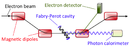
Figure 1: Design of the Hall A Compton polarimeter. The angles are exaggerated: the crossing angle between the electron and photon beams is 23 mrad.

The Compton photon source, which was upgraded from infrared ($\lambda=1064$ nm) to green ($\lambda=532$ nm) in 2010, provides linearly polarized laser light which is transformed to circular polarization using a remotely-controlled quarter-wave plate (QWP). The QWP is rotated by 90 degrees to switch between left- and right-circularly polarized laser light. The laser light is locked in resonance in the Fabry-Pérot cavity for ${\sim}90$ s, then the cavity is taken out of resonance while the QWP is rotated to switch polarizations. The out-of-resonance period lasts ${\sim}30$ s and is used for background determination, since, when the cavity is unlocked, there is negligible photon power at the Compton interaction point (CIP). The main background sources are beam-halo bremsstrahlung and synchrotron radiation.

The laser photon polarization is monitored on-line at the cavity exit by two powermeters, which measure the outputs of a Wollaston prism polarizing beam splitter. A QWP lies before the Wollaston prism. About once per day, the angle of this QWP is scanned and the corresponding power meter measurements are used to determine the laser polarization at the cavity exit. These measurements, in combination with a polarization transfer function from off-line absolute polarization measurements at the CIP and cavity exit, are used to determine the laser polarization state at the CIP, $P_{\gamma}$ [11]. The photon polarization is ${\sim}99\%$.

The scattered photons are detected in a newly installed Ce-doped $\text{Gd}_{2}\text{SiO}_{5}$ (GSO) photon calorimeter, discussed in Sec. 4. The scintillation photons are detected by a single photomultplier tube (PMT), and the resulting signals are integrated with a customized Flash Analog-to-Digital Converter (FADC), discussed in Sec. 5. The upgraded FADC DAQ allows for a photon-arm-only polarization measurement.

3 Integrating vs. Counting Modes

The Compton photon scattering asymmetry may be measured either by counting the number of scattered photons detected for each helicity state (determined by counting the number of detected PMT pulses which cross a chosen discriminator threshold), or by integrating the scattered photon signal for each helicity state (determined by integrating all of the charge collected from the PMT for each helicity state). An asymmetry over helicity states, as in Eq. 2, may then be calculated using either value.

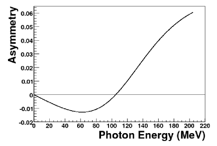
Figure 2: Theoretical Compton scattering asymmetry as a function of scattered photon energy for an electron beam energy of 3.4 GeV and a photon beam wavelength of 1064 nm. The maximum scattered photon energy for these kinematics is 204 MeV.

Fig. 2 shows the theoretical Compton asymmetry, $A_{th}$, plotted as a function of scattered photon energy for a 3.4-GeV electron beam and a photon wavelength of 1064 nm. A measurement weighted by the energy deposited by each Compton photon emphasizes the large-positive-asymmetry part of the curve while suppressing the negative-asymmetry part, and therefore enhances the measured asymmetry compared to simply counting the number of Compton photons detected for each helicity. Integration of the scattered photon signal yields an energy-weighted measurement.

There are several systematic uncertainties inherent in making either a counting or an integrating Compton polarization measurement, and these are considered below. The upgraded integrating DAQ design, however, eliminates several sources of systematic error from the original counting DAQ [12], and by carefully controlling the integrating DAQ systematics, a very precise measurement may be made.

Integration of the scattered-photon signal increases sensitivity to detector non-linearities, since any systematic distortion of the detected energy-deposited spectrum will also systematically distort the energy-weighted asymmetry. Integration also decreases the signal-to-background ratio compared to counting events above a discriminator threshold, which would essentially eliminate low-energy synchrotron radiation background. Sensitivities to pedestal fluctuations and scintillator afterglow are also increased. Detector non-linearities and scintillator afterglow can be controlled with careful detector design and study. Enhanced background and pedestal-fluctuation sensitivities increase the statistical error bar of the measurement, but are not a cause of systematic error, as long as background subtraction is done properly. Since the measurement is not statistics-limited, this increased statistical error is not a significant problem.

Signal integration, however, also eliminates sensitivities to threshold, pileup, and dead-time effects inherent in a counting measurement, which would be a potentially major source of systematic uncertainty. A no-threshold measurement also eliminates the need for precise calibration of the Compton photon spectrum (e.g. with the scattered electron energies measured by the Compton electron detector), which is required for the counting mode DAQ. This allows a precise stand-alone photon measurement to be made with the new integrating Compton DAQ.

4 Photon Detector

The new photon detector is a cylindrical GSO crystal that is 15 cm long and has a 6-cm diameter. It sits on a remotely-controllable table which can be moved horizontally and vertically; this is useful both for detector alignment and for moving the detector out of the beam when the background is very high. It has replaced the original photon detector, a 5$\times$5 array of 2 cm $\times$ 2 cm $\times$ 23 cm $\text{PbWO}_{4}$ crystals [13]. GSO has a fast and bright signal: it produces ${\sim}450$ optical photons per MeV (electron equivalent), with a stable signal width of ${\sim}85$ ns full width at half maximum. A typical photon pulse is shown in Fig. 3.

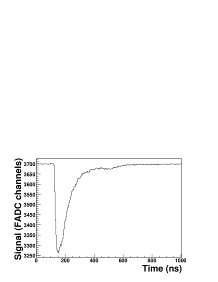
Figure 3: A GSO signal from an incident photon of ${\sim}$100 MeV. “Snapshot” taken using the triggered mode of the DAQ. The signal has a ${\sim}$1.1 V peak which corresponds to ${\sim}$10000 summed raw-ADC units (raus). Sampled voltage is reflected by a decrease from pedestal value.

The Hall A Compton photon beamline has also been modified, including the installation of a new collimator directly upstream of the photon detector. This collimator, which reduces bremsstrahlung background and defines the Compton angular acceptance, is a 5-cm-thick, 8-cm-diameter lead cylinder with a manually interchangeable aperture of 2 cm maximum diameter, located ${\sim}$6 m downstream of the CIP and ${\sim}$10 cm upstream of the GSO face.

A thin (0.25 to 8 mm thick, interchangeable), 4-cm-diameter lead disk is mounted on the downstream side of the collimator. This lead disk serves to shield the photon detector from low-energy synchrotron radiation background passing through the collimator aperture; the installed disk is chosen to be as thin as possible to achieve acceptable background rates, since the lead also stops low-energy Compton photons and introduces a distortion of the Compton spectrum which must be accounted for when calculating the experimentally relevant $A_{th}$.

4.1 Afterglow

Scintillator afterglow can affect the results of a Compton measurement, since long-term afterglow might last for multiple helicity cycles, or could even continue while the laser cavity is not locked and the background measurement is being made. The use of a scintillator that doesn’t have a long-term afterglow is therefore vital.

Douraghy et al. have measured a ${\sim}$5-$\mu$s afterglow in GSO [14], which is short compared to a 33-ms helicity window. Compton polarimeter data were also studied to confirm that any afterglow effect is negligible in this setup. A detector response due to afterglow would manifest as integrated signal that slowly decreases after beam trips (instead of falling immediately to zero) or as an increased integrated signal in those helicity windows which follow higher-rate helicity windows (an increase in signal in a window following an electron-photon helicity parallel window vs. an antiparallel one). No afterglow effect is distinguishable from statistical fluctuations in these studies, demonstrating that, in this instance, these effects are negligible.

4.2 Detector and Collimator Positioning

Kinematics relate photon energy and scattering angle for backscattered Compton photons:

$$k^{\prime}=\frac{4kE^{2}}{4kE+m^{2}+\theta_{\gamma}^{2}E^{2}}$$ (5)

in the lab frame, where $k$ and $k^{\prime}$ are the initial and scattered photon energies respectively, $E$ is the incident electron energy, $m$ is the electron mass, and $\theta_{\gamma}$ is the scattered photon angle. Lower-energy scattered photons have a larger deviation from the initial electron direction. Ideally, the collimator intercepts only the lowest-energy Compton photons; any mis-centering of the collimator causes some fraction of higher-energy photons to be intercepted. This mis-alignment must at the least be properly reflected in the GEANT4 simulation used to calculate $A_{th}$, and should be minimized, if possible. A mis-centered positioning of the GSO calorimeter may also result in photon-energy-dependent changes in energy-weighting which should also be included in $A_{th}$, although this effect is considerably less sensitive to small offsets than is the collimator position. Both effects can be minimized if the position of the center of the backscattered photon beam can be accurately determined (and the collimator and detector can be centered on it, if possible).

A position monitor has therefore been implemented: two 0.1 cm $\times$ 0.1 cm $\times$ 4.1 cm pieces of tungsten have been precisely positioned and bolted to the GSO housing upstream of the front face of the crystal, as shown in Fig. 4. One tungsten converter is placed horizontally, positioned 20 mm above the center of the GSO crystal; the other is placed vertically and is positioned 20 mm towards beam left from the center of the crystal. During normal data-taking, these lie out of the path of the Compton photons. The tungsten pieces sit in front of small bars of scintillator, which are read out by PMTs. When the tungsten converters intercept the photon beam they initiate showers, which are then detected by the scintillators.

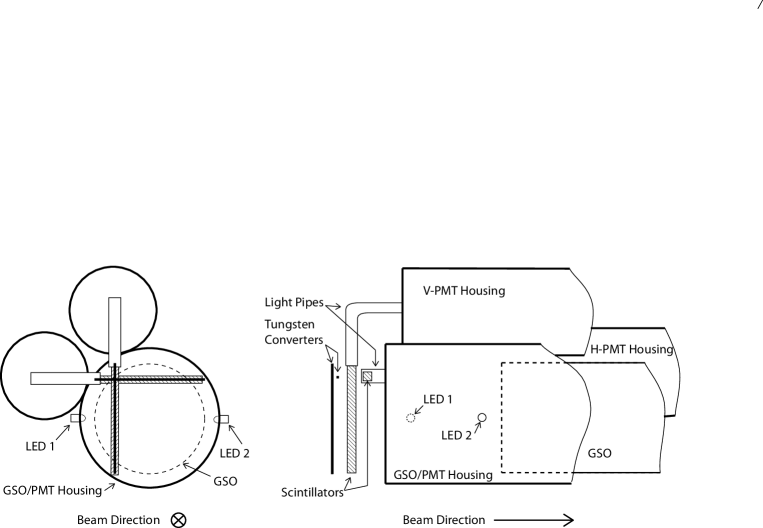
Figure 4: Front and side view of the GSO detector housing including the tungsten converters and scintillators used for determining the photon beam position. Here the V-PMT and H-PMT read out the vertical and horizontal converters respectively. The center of each converter bar is 20 mm away from the center of the GSO. LEDs placed in front of the detector, for use with the detector linearity test rig described in Sec. 4.3, are also shown.

Using the remotely controlled photon detector table, the position of which can be precisely set and read-back electronically to 0.2 mm, the detector may be moved while the electron beam is in the hall. The entire photon detector is scanned horizontally while centered vertically, and then scanned vertically while centered horizontally, and the trigger rate in the PMTs reading out each scintillator bar is monitored. When the tungsten converter crosses the scattered photon beam, the trigger rate increases notably. These tungsten converters can therefore be used to precisely determine the location of the scattered photon beam relative to the center of the GSO, and the photon detector table can be positioned accordingly.

The photon detector also has an attached precision-placed long metal “pointer”, which moves relative to a grid mounted on the side of the stationary collimator. This can be used to precisely determine the position of the photon beam at the collimator; the collimator can then be positioned manually so that the photon beam is centered on the collimator hole with a precision of ${\sim}$0.5 mm.

4.3 Detector Linearity Testing

Since an integrating asymmetry measurement is especially sensitive to detector non-linearities, as described in Sec. 3, a test rig [15] using light-emitting diodes (LEDs) has been designed and built in order to accurately determine the response of the PMT used to read out the GSO photon response pulses. This test rig also allowed the design of the PMT base to be fine-tuned to achieve good linearity and rate stability.

The precise results of the linearity measurement made using this device are an input into the GEANT4 simulation used to calculate $A_{th}$.

The LED test rig can also be used to monitor PMT rate-dependent gain shifts. For example, there is an observed 1% increase in gain for data taken in the presence of Compton signal plus background compared to that taken in the presence of just background during the HAPPEX-III experiment. This was measured by flashing an LED at a range of stable brightnesses while locking and unlocking the photon Fabry-Pérot cavity, and triggering the DAQ on the same trigger as the LED. After taking pileup effects into account, any systematic difference in LED pulse size between cavity-locked and cavity-unlocked states is due to a detector gain shift. This effect can then be accounted for during analysis.

5 Data Acquisition System

The upgraded integrating data acquisition system is based upon the 200 MHz Struck SIS3320 12-bit VME FADC. The FADC continuously samples the photon detector PMT output at 200 MHz (using an external 40 MHz clock internally converted to 200 MHz). The FADC sums the sampled data into six 36-bit accumulators, which sum ADC values between an external $T_{start}$ and $T_{stop}$ signal. This accumulator mode is implemented through a customization of the FADC, as described in Sec. 5.1. Simultaneously, the FADC stores all of the samples for a single helicity window as sequential entries in one of two internal buffers. The buffer is switched after each helicity window. A selected number of samples of the stored data can be read out for each of a limited number of triggers in triggered-mode running, as described in Sec. 5.2.

Necessary diagnostic signals, such as readback from beam current and position monitors in the Compton beamline and the measured power of photons transmitted through the Compton cavity, are converted to frequency signals in a voltage-to-frequency converter, and are sent to two CAEN V560 scalers. The scalers are read out every helicity window, so that cuts on these quantities can be made on a window-by-window basis during data analysis. Other quantities, such as trigger rates and clock pulses, are also counted by these scalers.

Figure 5: Timing structure for helicity windows. The timing signals are not drawn to scale, since the values of $T_{settle}$, $T_{stable}$, and the integration time are selectable.

The timing structure for the DAQ is shown in Fig. 5. The external $T_{start}$ and $T_{stop}$ signals are generated using a customized VME Timing Board [16]. This VME module takes the accelerator helicity timing signal (called the MPS signal) as a TTL input, outputs the $T_{start}$ signal a programmable interval of at least 15 $\mu$s later, and outputs the $T_{stop}$ signal a programmed interval after the $T_{start}$ signal. The time between the $T_{start}$ and $T_{stop}$ signals must be set to less than the length of the accelerator’s helicity window. Data readout is initiated by the $T_{stop}$ signal, and the time period between $T_{stop}$ and the next $T_{start}$ is used to read out the accumulator and scaler data. The triggered data can be read out during the following helicity window, since the samples for two adjacent windows are stored in two separate buffers. Since the time between $T_{start}$ and $T_{stop}$ is completely programmable, the integrating DAQ can be run at any accelerator helicity-flip period.

5.1 Accumulator Mode

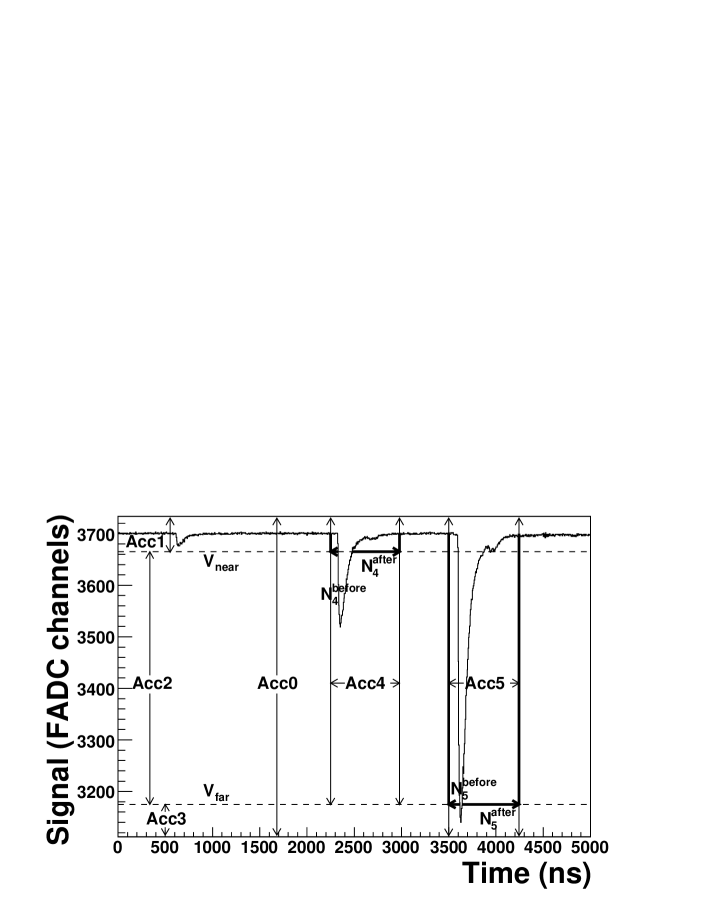
Figure 6: The six accumulators are represented schematically. Signal size within a sample is represented by a decrease in value from a pedestal value.

There are six accumulators, represented in Fig. 6, which are read out for each helicity window:

• Accumulator 0 (All) sums all samples between the external $T_{start}$ and $T_{stop}$ signals.

• Accumulator 1 (Near) sums all samples that fall closer to the pedestal than a threshold near the pedestal, $V_{near}$ (low-energy photons).

• Accumulator 2 (Window) sums all samples between $V_{near}$ and a threshold far from the pedestal, $V_{far}$ (with $V_{near}$ between the pedestal and $V_{far}$).

• Accumulator 3 (Far) sums all samples beyond $V_{far}$ (the tips of pulses from high-energy photons past the Compton edge).

• Accumulator 4 (Stretched Window) sums starting a set number of samples, $N_{4}^{\mathit{before}}$, before the signal crosses $V_{near}$, and continues to integrate until another set number of samples, $N_{4}^{\mathit{after}}$, after the signal crosses $V_{near}$ again, except that samples which are included in accumulator 5 are not included in accumulator 4.

• Accumulator 5 (Stretched Far) sums starting a set number of samples, $N_{5}^{\mathit{before}}$, before the signal crosses $V_{far}$, and continues to integrate until another set number of samples, $N_{5}^{\mathit{after}}$, after the signal crosses $V_{far}$ again.

The All, Window, and Stretched Window accumulators are intended as possible measures of Compton signal, while the Near, Far, and Stretched Far accumulators are intended primarily for use in understanding backgrounds.

The goal of the Stretched Window accumulator is to include the entire Compton pulse, while excluding low-energy background pulses and the entirety of high-energy background bremsstrahlung pulses (which go into the Stretched Far accumulator).

The number of samples summed into each accumulator for each helicity window is also read out. This is necessary for pedestal subtraction during analysis.

5.2 Triggered Mode

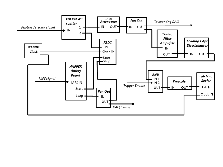
Figure 7: Simplified schematic of the upgraded integrating Compton DAQ.

To allow for study of individual pulse integrals and shapes, a sampled triggered mode is implemented in parallel with the accumulator mode. For the triggered mode, while the detected pulse shape is continuously sampled by the FADC, the clock times of an external trigger are recorded in a CAEN V830 latching scaler. The latching scaler counts clock ticks and accepts an external trigger; when it receives a trigger, it stores the current clock counter for subsequent readout. During readout after the end of the helicity window, a programmable sampling period, usually 500 ns, is read out from the FADC memory for each latched trigger time, starting some programmable interval before the stored trigger time, in order to also read out the pulse shape before the trigger. The samples making up the pulse can then be summed numerically (with only this sum being written into the datastream), or all of the samples for a single trigger can be saved to the datastream. The readout time for either method is equivalent, but writing out individual samples requires considerably more disk space. Therefore, most triggered pulses are integrated, and only a few fully sampled triggered pulses are written out for each helicity period.

There is a concern with readout time: because the data are stored in alternating buffers, the DAQ must be finished reading out the triggered data by the end of the subsequent helicity period. Also, since the scaler information is not buffered, the diagnostic scalers and all the trigger times must be read during the short interval between $T_{stop}$ and $T_{start}$. The number of trigger times stored and the number of samples read out must therefore be limited so that the DAQ is finished reading out before the data are overwritten. Limits are therefore placed on the number of samples stored, and the GSO photon trigger is prescaled (using a remotely controllable CAEN V1495, programmed to work as a prescaler) before being sent to the latching scaler. Prescaling allows the latched triggers to be distributed across the helicity window, in order to monitor any systematic signal variation as a function of time within the helicity window.

The latching scaler must run on the same clock as the FADC, or the two sampling rates may drift with respect to one another, causing the trigger times stored in the latching scaler to become incorrect. Although the CAEN V830 latching scaler is specified to accept clocks up to 250 MHz, the NIM output signal of the internal FADC clock was found to be unable to properly trigger the scaler at such high rates. The latching scaler clock input is therefore the same external 40 MHz clock used by the FADC. There is a drawback to this method: the coarse clock on the latching scaler causes some jitter in the trigger times.

A set of NIM logic gates, controlled via programmable output bits from the Trigger Interface Register (TIR) of the DAQ, allows the trigger input to the V830 to be remotely selected. The standard trigger is, of course, the signal from the photon detector. This is split by a 4:1 passive splitter; the majority of the signal is sent directly to the FADC, and the rest is attenuated, sent through a Timing Filter Amplifier (TFA) for shaping, and then to a discriminator with a very low threshold. A prescaled sample of the pulses which fire the discriminator are sent to the latching scaler. Use of a passive splitter for the photon signal going into the FADC is important, to avoid introducing a rate-dependent gain shift. For example, a significant (2.5 mV) gain shift effect was seen in the TFA when going between trigger rates with the cavity locked compared to with the cavity unlocked with a 100 $\mu$A electron beam. A schematic of the DAQ is shown in Fig. 7.

A remotely programmable (nominally 1 kHz) square pulse, either in coincidence with an LED pulser, or alone for looking at samples uncorrelated to pulses, can also be used as a trigger. The photon DAQ can also be triggered on the Compton electron detector signal, allowing analysis of electron/photon coincidences.

The standard triggered-running mode reads Compton photon detector triggers for three helicity windows, and then reads out random samples every fourth helicity window. The random samples are chosen in the readout code by stepping through the length of the helicity window. These random samples are used for background and pileup analysis.

A Compton photon energy spectrum, measured using the summed triggered mode of the DAQ, is shown in Fig. 8, where the horizontal axis is ADC response due to energy deposited in the GSO in summed raw-ADC units (raus). A plot of the measured Compton asymmetry as a function of ADC response is shown in Fig. 9. These triggered spectra have been fit using the shapes predicted by the GEANT4 Monte Carlo (MC) used to calculate $A_{th}$. This MC includes information about the electron and photon beam energies; the detector and collimator position relative to the photon beam, as discussed in Sec. 4.2; the detector linearity, as discussed in Sec. 4.3; pileup effects; and smearing effects due to photoelectron statistics and light collection in the detector.

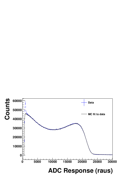
Figure 8: A measured Compton photon energy spectrum. The triggered data is fit to GEANT4 MC data with only two free parameters: a horizontal scale factor and a vertical scale factor. A smearing factor which accounts for PMT and DAQ resolution, as well as GSO light collection, is also included. The fit is good enough that the data and MC fit are indistinguishable, except at low photon energies, where the triggered-data background-subtraction (which is done absolutely by taking beam current and trigger rates into account) is incorrect due to a rate-dependent gain shift of the TFA, which causes a trigger-discriminator threshold shift.

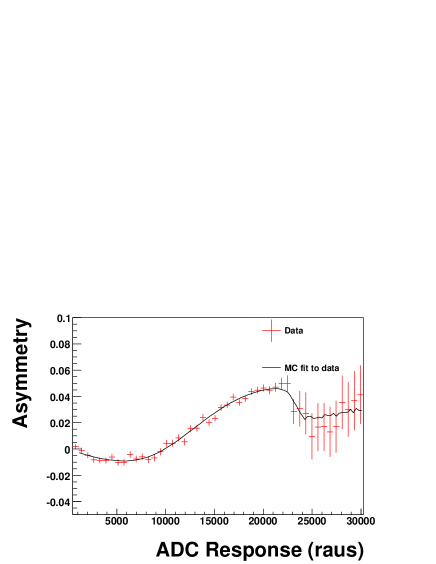
Figure 9: The measured Compton asymmetry plotted against ADC response due to energy deposited in the GSO. The triggered data is compared to GEANT4 MC data with no adjustable parameters. (The horizontal scale is taken from the fit from Fig. 8 and the vertical scale is set by the measured $P_{e}$ and $P_{\gamma}$.)

6 Integrating-Data Analysis

Extracting an electron beam polarization from accumulator data requires making cuts to the data based on parameters such as electron beam current and photon cavity power. An asymmetry can then be calculated in several different ways; an accumulator (Sec. 6.1) and method of asymmetry calculation (Sec. 6.2) must be chosen based on which measurement gives the lowest error. Statistical (Sec. 6.2.1) and systematic (Sec. 6.3) errors on the asymmetry must then be calculated.

Since the FADC actually stores the signal as offsets below the pedestal value, as in Fig. 3, the integrated signal for each window is calculated as

$$S_{n}=N_{n}\bar{P}-Acc_{n},$$ (6)

where $S_{n}$ is the physics signal extracted from the $n$th FADC accumulator, $N_{n}$ is the number of samples that have been summed into the accumulator, $\bar{P}$ is the best estimate of the average pedestal value for each sample, and $Acc_{n}$ is the integrated ADC value for the helicity window.

The accumulator values are used to calculate the asymmetry $A_{exp}$ from Eq. 2: for each period of right- or left-circular laser polarization, separate sums of accumulator values for all positive- and negative-helicity windows are made. A sum is also made of accumulator values for the adjacent cavity-unlocked periods, to determine background, $B$, for the cavity-locked period. The measured asymmetry needs to take into account the background, such that Eq. 2 becomes

$$A_{exp}=\frac{(\langle M^{+}\rangle-\langle B\rangle)-(\langle M^{-}\rangle-\langle B\rangle)}{(\langle M^{+}\rangle-\langle B\rangle)+(\langle M^{-}\rangle-\langle B\rangle)},$$ (7)

where $\langle\rangle$ denotes the mean accumulator value per helicity window over each cavity (-locked or -unlocked) period. Here, $M^{+(-)}$ is the measured integrated signal plus background for positive (negative) helicity electrons (where $S=M-B$). $A_{exp}$ is calculated separately for each laser polarization. It is assumed in this calculation that $B^{+}=B^{-}$, which is true as long as the electron beam parameters (such as beam position and charge) are carefully kept helicity-independent. This helicity independence is also necessary for making a Compton polarization measurement with better than 1% systematic error, as well as for performing parity-violation measurements [17]. The background then cancels in the numerator of Eq. 7.

Since $N_{n}$ is always the same for every helicity window in the All accumulator (independent of the state of the helicity or laser cavity), $N_{n}\bar{P}$, from Eq. 6, therefore cancels in both the numerator and denominator of Eq. 7, and an All accumulator measurement is insensitive to the choice of pedestal value. The same is not true of accumulators with thresholds.

6.1 Analysis with Threshold Accumulators

Using the threshold accumulators (Window or Stretched Window accumulators) for Compton data analysis increases signal-to-noise but comes with an inherent additional systematic error, and therefore must be done with care: one main advantage of making an integrating measurement is the elimination of thresholds; when thresholds are reintroduced, these systematics return.

Since $V_{near}$ may be placed very close to the pedestal and the measurement is energy-weighted, introducing a threshold does not have a large effect on $A_{exp}$ to first order. However, complicated pileup effects can distort the measured asymmetry, since small background pulses that do not cross $V_{near}$ when the cavity is in the unlocked state, may cross $V_{near}$ when they pile up with Compton photon pulses.

The main additional systematic effect that comes from using a threshold accumulator, however, is a sensitivity to the accurate determination of the pedestal value, $\bar{P}$. Since the raw accumulator data must be pedestal-subtracted, as in Eq. 6, and background-subtracted, as in Eq. 7, and there are a different number of samples in each helicity window (specifically when the cavity is locked vs. unlocked), the result is sensitive to the value of $\bar{P}$. Since the FADC pedestal is not stable (slow drifts of the pedestal on the order of ${\sim}$0.1 channels in hours or ${\sim}$0.4 channels in weeks have been observed), it is very difficult to subtract the correct pedestal value. Systematic errors introduced due to a 0.4 channel pedestal uncertainty are around 0.5-1%, depending on the relative signal-to-background rates. Reduction of this systematic error could be achieved by shutting off the electron beam or detector high voltage every few hours during data-taking, in order to monitor the pedestal, but this imposes significant overhead, and still does not solve the problem for shorter-timescale pedestal drift.

Use of a threshold also introduces a second-order distortion in the measured energy-weighted asymmetry, since $V_{near}$ discards a larger fraction of each lower-energy photon pulse which crosses it compared to higher-energy pulses in the Window accumulator. The Stretched Window accumulator is more complicated, since it opens a window which integrates $N_{4}^{\mathit{after}}$ samples after the signal re-crosses the threshold, and the timing of the threshold-crossing walks depending on the photon energy (again causing a distortion in the energy-weighted asymmetry). Because of the fast rise-time of each photon pulse, this is not a problem for the initial threshold crossing in the Stretched Window accumulator. To improve understanding of the Stretched Window accumulator data and facilitate better extraction of a polarization from this data, a future version of the SIS3320 firmware would stop counting $N_{4}^{\mathit{after}}$ after $V_{near}$ was crossed the first time, instead of the second time, thereby integrating the same number of samples for each pulse, independent of the pulse height. The same would be done for the Stretched Far accumulator and $N_{5}^{\mathit{after}}$.

These effects cause a non-negligible systematic difference in the measured asymmetry for each accumulator (e.g. the measured asymmetry for HAPPEX-III is systematically 0.3% higher in the Stretched Window accumulator relative to the All accumulator and is 1.1% higher in the Window accumulator relative to the All accumulator), and must therefore be taken into account when calculating $A_{th}$.

The use of the All accumulator was therefore found to produce results with smaller overall systematic errors, since it is better understood.

6.2 Asymmetry Calculation

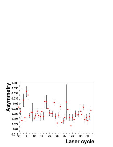
(a)

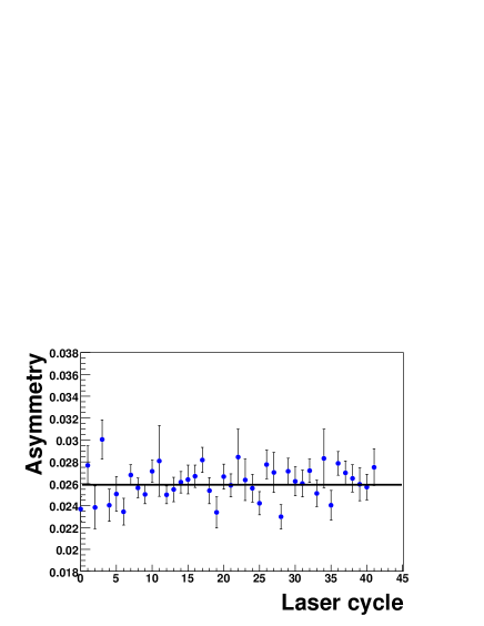
(b)

Figure 10: A typical Compton slug for (a) laser-right and (b) laser-left, where the absolute value of the asymmetry has been taken. Each data point is a separate laser-cycle including local background subtraction. Error bars are statistical as defined in Sec. 6.2.1. The solid line is a constant fit to the data.

There are several options for extracting an asymmetry (calculated as in Eq. 7) from the Compton accumulator (All, Window, or Stretched Window) data. Three options discussed here are called laser-wise, for which an asymmetry is calculated for each laser cycle; run-wise, for which an asymmetry is calculated for each one- or two-hour long run; and pair-wise, for which an asymmetry is calculated for each helicity pair.

The laser-wise method of extracting an asymmetry involves calculating a separate mean of the accumulated value (averaged over the number of helicity windows) of all helicity-plus and -minus windows for each cavity-locked period, as described in Sec. 6. A mean local background from the two cavity-unlocked periods adjacent to the cavity-locked period is also calculated. Since the background contributions to signal fluctuate quickly and tend to drift on the timescale of minutes, local background determination is advantageous. A separate statistical error bar is then assigned for each laser-cycle point (as described in Sec. 6.2.1), and the points are collected into ${\sim}$50 laser-cycle-long “slugs” of data (broken up so that no run is divided between multiple slugs and each slug contains two long runs or several short runs with no configuration changes). Measured asymmetries from a typical slug are shown in Fig. 10. The mean for each slug is taken as a separate data point (as plotted in Sec. 7). This method appears to have the best balance of consistency checks and resistance to excessive noise, and was used to determine the electron beam polarization for the HAPPEX-III measurement.

The data can also easily be broken up into runs: a sum and a difference for each (${+}{-}$) helicity pair in the run is calculated (separately for each laser polarization, of course), and the mean of these values is taken over the entire run. A mean background value for the entire run is also calculated. These numbers are then used as the numerator and denominator in Eq. 7. Histograms of the sum, difference, and background for a typical run are shown in Fig. 11. This run-wise method of calculating the asymmetry is particularly useful for running at lower rates: since each (${\sim}$90 s) laser-cycle has low photon statistics at low rates, doing a laser-wise analysis is impossible. This method has the disadvantage that the background level is averaged over the entire run, which significantly increases the error due to background subtraction when backgrounds are unstable.

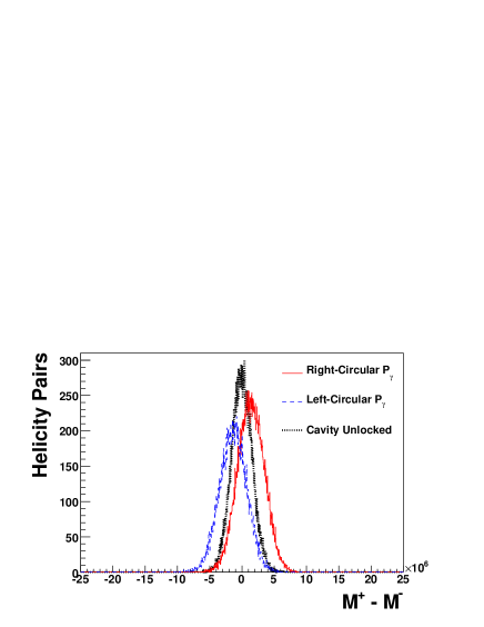
(a)

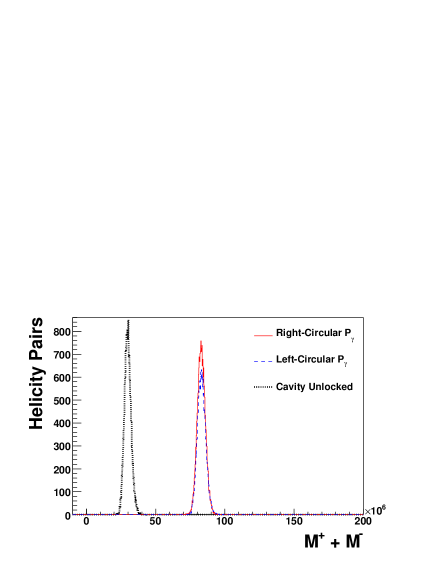
(b)

Figure 11: Histograms of the (non-background-subtracted) (a) numerator and (b) denominator of the Compton asymmetry for an entire two hour long run.

The pair-wise method involves calculating a separate (background-subtracted) asymmetry, as shown in Fig. 12, for each helicity pair. Preliminary results using this method are described by Parno et al. [18]. The simplest implementation of this method also uses a background calculated for the entire run, and so a run-averaged background value is subtracted rather than a local one. Calculating an error bar for this method requires use of not only the statistical error on the distribution from Fig. 12, but also the statistical error on the background spectrum. Unfortunately, when the background is high and unstable (with an integrated background to signal ratio of more than ${\sim}$1 or a background distribution RMS width of more than ${\sim}10\%$ of the mean), the pair-wise distribution becomes non-Gaussian, and therefore this method does not give correct statistical errors nor mean asymmetries.

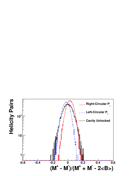
Figure 12: Histogram of a background-subtracted Compton asymmetry taken for every pair in a single two hour long run.

6.2.1 Calculation of Statistical Errors

To assign statistical error bars when calculating a run-wise or laser-wise asymmetry, the RMS width of each sum, difference, and background distribution (as shown in Fig. 11 for a whole run, but done separately for each laser-cycle for a laser-wise analysis) is divided by the square root of the number of data points. This quantity for the sum, difference, and twice the background is labeled $\sigma_{S}$, $\sigma_{D}$, and $\sigma_{B}$ respectively. These values are then used to calculate a statistical error on each point, treating $\langle M^{+}-M^{-}\rangle$, $\langle M^{+}+M^{-}\rangle$, and $\langle 2B\rangle$ as independent variables in Eq. 7:

$$\sigma^{2}= \frac{\sigma_{D}^{2}}{(\langle M^{+}\rangle+\langle M^{-}\rangle-2\langle B\rangle)^{2}}+$$

$$\frac{(\sigma_{S}^{2}+\sigma_{B}^{2})^{2}(\langle M^{+}\rangle-\langle M^{-}\rangle)^{2}}{(\langle M^{+}\rangle+\langle M^{-}\rangle-2\langle B\rangle)^{4}}.$$ (8)

This method of error calculation allows the width of the background distribution to be properly taken into account when assigning errors.

A table of the average All accumulator sum and difference values and the RMS widths of the distributions measured during the HAPPEX-III experiment is given in Sec. 7.

6.3 Calculation of Systematic Errors on the All Accumulator

As long as the electron beam parameters are kept minimally helicity dependent, the main systematic error on an All accumulator integrating Compton asymmetry is due to the observed PMT gain shift between cavity-locked and -unlocked states. The systematic error due to the gain shift results from uncertainty in the size of the gain shift itself (the signal-to-background ratio during a three-month-long experiment does not stay constant, and the gain shift changes depending on the relative rates). There is also an error on the gain shift due to pedestal uncertainty, since a gain shift correction is implemented (by scaling $\langle B\rangle$ in Eq. 7) after pedestal subtraction, and is therefore sensitive to the correct assignment of the pedestal value, which no longer cancels exactly, even for the All accumulator.

A pedestal shift between cavity-locked and -unlocked states would also be a source of systematic error, but there is no such observed pedestal shift in this setup.

Systematic errors in the analyzing power must also be calculated, and these are estimated by changing the beamline and electron beam parameters input into the GEANT4 MC, e.g. the photon beam position on the collimator or the electron beam energy, over the experimentally possible range of values, and measuring the fractional change in $A_{th}$. There is also a systematic error on $A_{th}$ due to detector non-linearity: the detector linearity is measured as described in Sec. 4.3, and this measured value is input into the MC. The systematic error on $A_{th}$ due to non-linearities is then estimated by tweaking the non-linearity input into the MC and monitoring the effect of these changes on the fit of the MC data to the Compton spectrum, as in Fig. 8, as well as the effect on $A_{th}$.

A table of systematic errors on the Compton integrating measurement for the HAPPEX-III experiment is given in Sec. 7.

7 Measurement Results

The upgraded photon arm of the Compton polarimeter was used to continuously measure the CEBAF electron beam polarization during several experiments, including HAPPEX-III, which ran in 2009. This particular measurement achieved a 0.94% relative (0.84% absolute) systematic error, which mostly came from an uncertainty in laser photon polarization in the cavity. As discussed in Sec. 2, the photon polarization is determined by combining an on-line measurement of the polarization at the cavity exit with a measurement of the cavity transfer function; there is a 0.8% error on the cavity transfer function measurement. The systematic errors on the asymmetry measurement are detailed in Sec. 6.3. The breakdown of Compton systematic errors is shown in Table 1.

Systematic Errors
Laser Polarization	0.80%
Analyzing Power:
Non-linearity	0.3%
Electron Energy Uncertainty	0.1%
Collimator Position	0.05%
MC Statistics	0.07%
Total on Analyzing Power	0.33%
Gain Shift:
Background Uncertainty	0.31%
Pedestal Uncertainty	0.20%
Total on Gain Shift	0.37%
Total	0.94%

Table 1: Breakdown of Compton systematic errors using the All accumulator during HAPPEX-III.

The statistical error after three months of HAPPEX-III running with the integrating Compton DAQ was 0.06%. Statistical error calculation is discussed in Sec. 6.2.1, and a table of the measured means and RMS widths of the (non-background-subtracted) sum and difference distributions from the All accumulator for each run, averaged over all of the HAPPEX-III runs, is given in Table 2. The means and RMS widths of the background and pedestal are also given.

Measurement	Mean (raus)	RMS Width (raus)
Sum	$124\times 10^{6}$	$13\times 10^{6}$
Difference	$1.8\times 10^{6}$	$5.5\times 10^{6}$
Background	$54\times 10^{6}$	$16\times 10^{6}$
Pedestal	$24000\times 10^{6}$	$0.71\times 10^{6}$

Table 2: The measured means and RMS widths of the non-background-subtracted sum and difference distributions from the All accumulator for each run, as in Fig. 11, averaged over all of the HAPPEX-III runs (with ${\sim}90\times 10^{3}$ MPSs in each run). The means and RMS widths of the background (summed over pairs of windows) and pedestal (for single 33 ms helicity windows) are also given.

Because there were gaps in the run period during which the polarization was not monitored by the Compton polarimeter (due in part to electron beam instability which made Compton measurements impossible and in part to a period of time for which the laser polarization became unknown due to an equipment failure), an additional error of 0.2% was included.

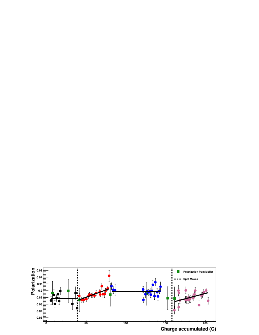
Figure 13: A plot of measured polarization vs. HAPPEX-III charge accumulated. The round points are measured using the Compton polarimeter integrating DAQ, and error bars are statistical only. The vertical dashed lines mark when the laser spot was moved at the accelerator source, and the solid lines are linear fits to the Compton data, where the HAPPEX-III run period is broken into four distinct polarization periods and fit accordingly. The square points are from the Hall A Møller polarimeter [19], and the error bars on these points include a 1.7% systematic error.

A plot of the electron polarization as a function of HAPPEX-III incident beam charge accumulated is shown in Fig. 13. In this plot, the vertical dashed lines mark when the laser spot was moved at the accelerator source; there is a distinct measured change in polarization behavior following spot moves [20]. The observed gradual increase in polarization following spot moves is consistent with a gradual degradation of the photocathode surface, which has been observed to increase electron polarization while the quantum efficiency drops [22, 21]. The photon arm of the Compton polarimeter has measured the average beam polarization over the HAPPEX-III run to be $[89.41\pm 0.05(\text{stat})\pm 0.84(\text{sys})\pm 0.18(\text{gaps})]\%$.

8 Conclusion

The photon arm of the Jefferson Lab Hall A Compton polarimeter has been upgraded with a new integrating DAQ and photon detector. These have been used to determine the beam polarization during HAPPEX-III with better than 1% total error at 100 $\mu$A electron beam current and 3.4 GeV electron beam energy. These results agree with concurrently running Møller polarimeter measurements, but have higher precision. Polarization measurements made using the upgraded Compton DAQ and photon detector also show a marked improvement compared to those made with the original apparatus, with an overall error improved by about a factor of three.

The upgraded Compton photon arm has been used in several experiments which have run in Hall A since 2009 in addition to HAPPEX-III: d${}_{2}^{n}$ [23], PVDIS [24], PREX [25], and DVCS [26]. Future Hall A parity experiments, such as the MOLLER [27] and SoLID [28] experiments, also require electron beam polarimetry with sub-1% precision and will use an integrating Compton photon DAQ. A similar integrating DAQ was also installed in the new Hall C Compton polarimeter at Jefferson Lab in 2010 for use in the $Q_{weak}$ experiment [29].

Results obtained using the upgraded photon arm of the Hall A Compton polarimeter can be compared to results obtained with Compton polarimeters used at lower electron beam energies at NIKHEF [30] and MAMI [31] (which quote 2.7% and 2% absolute systematic errors respectively), and at higher electron beam energies at HERA [32] and SLAC [33] (which quote 1.6% relative and 0.5% absolute systematic errors respectively).

References

- [1] C.W. Leemann, D.R. Douglas and G.A. Krafft, Annu. Rev. Nucl. Part. Sci. 51 (2001) 413.
- [2] S. Escoffier et al., Nucl. Instr. and Meth. A 551 (2005) 563.
- [3] J.P. Jorda et al., Nucl. Instr. and Meth. A 412 (1997) 1.
- [4] F.W. Lipps and H.A. Tolhoek, Physica 20 (1954) 85.
- [5] C.Y. Prescott, SLAC preprint TN-73-1 (1973).
- [6] K.A. Aniol et al., A measurement of nucleon strange form factors at high , Proposal for Jefferson Lab PAC 29, 2005.
- [7] S. Agostinelli et al., Nucl. Instr. and Meth. A 506 (2003) 250.
- [8] D. Parno, Measurements of the double-spin asymmetry A1 on helium-3: Toward a precise measurement of the neutron A1, PhD thesis, Carnegie Mellon University, 2011.
- [9] A. Denner and S. Dittmaier, Nucl. Phys. B 540 (1999) 58.
- [10] JLab Hall A preprint, (2004), http://hallaweb.jlab.org/parity/prex/compton_upgrade.pdf.
- [11] M. Baylac, Measurement of the polarization of the electron beam at Jefferson Laboratory via the Compton effect, for the HAPPEX experiment to measure parity violation in elastic electron-proton scattering [in French], PhD thesis, Université Claude Bernard-Lyon 1, 2000.
- [12] M. Baylac et al., Phys. Lett. B 539 (2002) 8.
- [13] D. Neyret et al., Nucl. Instr. and Meth. A 443 (2000) 231.
- [14] A. Douraghy et al., Nucl. Instr. and Meth. A 569 (2006) 557.
- [15] M. Friend, G.B. Franklin and B. Quinn, submitted to Nucl. Instr. and Meth. A (2011), arXiv:1108.3096.
- [16] G.W. Miller, Parity violation in forward angle elastic electron-proton scattering, PhD thesis, Princeton University, 2001.
- [17] K.D. Paschke, European Physical Journal A 32 (2007) 549.
- [18] D. Parno et al., Proceedings of the 2010 International Nuclear Physics Conference, Journal of Physics: Conference Series, 2010, arXiv:1106.4851, in press.
- [19] D.S. Dale et al., Polarized Gas Targets and Polarized Beams: Seventh International Workshop: Urbana, IL, August 1997, edited by R. Holt and M.A. Miller, pp. 321–325, Springer-Verlag New York, LLC, 1998.
- [20] C.K. Sinclair et al., Phys. Rev. Spec. Top. Accel. Beams 10 (2007) 023501.
- [21] P. Sàez, SLAC preprint SLAC-R-501 (1997).
- [22] H. Tang et al., The International Workshop on Polarized Beams and Polarized Gas Targets Vol. SLAC-PUB-6918, SLAC, 1995.
- [23] X. Zheng et al., Precision measurement of the neutron : Towards the electric and magnetic color polarizabilities, Proposal for Jefferson Lab PAC 29, 2005.
- [24] A. Afanasev et al., H Parity Violating Deep Inelastic Scattering (PVDIS) at CEBAF 6 GeV, Proposal for Jefferson Lab PAC 33, 2007.
- [25] K.A. Aniol et al., A clean measurement of the neutron skin of 208Pb through parity violating electron scattering, Proposal for Jefferson Lab PAC 29, 2005.
- [26] C. Camacho et al., Complete separation of deeply virtual photon and electroproduction observables of unpolarized protons, Proposal for Jefferson Lab PAC 31, 2006.
- [27] J. Benesch et al., An ultra-precise measurement of the Weak Mixing Angle using Moller scattering, Proposal for Jefferson Lab PAC 34, 2008.
- [28] P. Bosted et al., Precision measurement of parity-violation in deep inelastic scattering over a broad kinematic range, Proposal for Jefferson Lab PAC 35, 2009.
- [29] D. Armstrong et al., The experiment: ‘A search for new physics at the TeV scale via a measurement of the proton’s weak charge’, Proposal for Jefferson Lab PAC 33, 2007.
- [30] I. Passchier et al., Nucl. Instr. and Meth. A 414 (1998) 446.
- [31] J. Diefenbach et al., Eur. Phys. J. A 32 (2007) 555.
- [32] M. Beckmann et al., Nucl. Instr. and Meth. A 479 (2002) 334.
- [33] SLD collaboration, M. Woods, The Workshop on High Energy Polarimeters at NIKHEF Vol. SLAC-PUB-7319, SLAC, 1996.