Effects of Mirror Aberrations on Laguerre-Gaussian Beams in Interferometric Gravitational-Wave Detectors

Abstract

A fundamental limit to the sensitivity of optical interferometers is imposed by Brownian thermal fluctuations of the mirrors’ surfaces. This thermal noise can be reduced by using larger beams which “average out” the random fluctuations of the surfaces. It has been proposed previously that wider, higher-order Laguerre-Gaussian modes can be used to exploit this effect. In this article, we show that susceptibility to spatial imperfections of the mirrors’ surfaces limits the effectiveness of this approach in interferometers used for gravitational-wave detection. Possible methods of reducing this susceptibility are also discussed.

I Introduction

Long-baseline laser-interferometer gravitational-wave detectors, such as those used in LIGO LIGO , VIRGO Virgo , GEO600 GEO and LCGT LCGT , use Michelson interferometry to measure tiny differential changes in arm length induced by gravitational waves. Spurious motions of a mirror’s surface, such as those caused by seismic, thermal, and radiation-pressure fluctuations, can compromise the sensitivity to gravitational wave signals. Brownian thermal noise in the dielectric mirror coatings, or coating Brownian noise, is known to be the dominant noise source in the intermediate frequency band of Advanced LIGO Harry:CoatingThermal and other similar interferometers.

As described by the Fluctuation-Dissipation Theorem Callen:FDT ; Levin:FDT , dissipation via internal friction in the dielectric coatings must lead to fluctuations in the thickness of the coatings. When the beam spot size is much larger than the coating thickness, coating Brownian noise at different locations on the mirror’s surface can be considered to be uncorrelated. This leads to the following scaling law Lovelace:thermal ; O'Shaugnessy:beam ,

$$S_{x}\propto\frac{\displaystyle\int I^{2}(\vec{r})\,\mathrm{d}^{2}\vec{r}}{\displaystyle\left[\int I(\vec{r})\,\mathrm{d}^{2}\vec{r}\right]^{2}}$$ (1)

which describes how the power spectrum of observed coating Brownian noise $S_{x}$ depends on the intensity profile $I(\vec{r})$ of the optical field which is used to read out the mirror motion; i.e. the coating Brownian noise power spectrum is inversely proportional to the effective area of the optical mode.

Table 1: Beam shapes that have been considered for use in gravitational-wave detectors, mirror shapes that support them and their thermal-noise suppression factors (in power) for Advanced LIGO parameters (cavity length $L=4$ km, mirror radius of 17 cm).

Mode	Mirror Shape	Suppression Factor	Ref.
LG3,3	Spherical	1.61	LG
Mesa	Sombrero	1.53	Bondarescu:Mesa ; Miller:Thesis
Conical	Conical	2.30	conical

Three families of optical modes have so far been considered for mitigating coating thermal noise (see Table 1). Among these modes, only the higher-order Laguerre-Gauss mode, LG_3,3, can be supported by optical cavities employing standard spherical mirrors. Due to the practical advantages associated with the use of spherical mirrors, experimental testing of LG_3,3 modes has begun. It has thus far been demonstrated that these modes can be generated with high efficiency and resonated in tabletop cavities with small mirrors Fulda:LG ; Matteo:LG .

An unpleasant property of higher-order LG modes is that each LG_p,l mode is $2p+|l|+1$-fold degenerate, the LG_3,3 mode being 10-fold degenerate. Mirror figure errors will inevitably split each formerly degenerate mode into $2p+|l|+1$ single modes with eigenfrequencies which depend on the particulars of the figure error. By contrast, a non-degenerate mode, under the same figure error, will usually remain as a single, weakly-perturbed non-degenerate mode.

In this work we explore the effects of LG_3,3 modal degeneracy quantitatively, via both numerical and analytical methods. Guided by experience with existing interferometers we have selected contrast defect as our metric of interferometer performance.

To ground our investigation in reality we incorporate mirror figure errors derived from measurements of the first Advanced LIGO optics. The creation of these maps is described in Section II.

In Section III, we use perturbation theory to analyze the effect of such mirror perturbations on the degenerate subspace which includes the LG_3,3 mode. We then use this newly perturbed set of modes to calculate the contrast degradation of a single Fabry-Perot arm cavity analytically in Section IV.1.

In Section IV.2, we utilize a sophisticated numerical field propagation code to confirm analytical results and examine a more complicated interferometer topology.

In Sec. V, we explore two methods of mitigating contrast degradation; neither of the methods was ultimately successful.

II Mirror Figure Errors

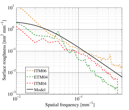
Figure 1: Power spectral densities of uncoated mirror surface roughness. The dashed lines are the measured spectra of three Advanced LIGO arm cavity mirrors. A model approximating these spectra (black trace, see (2)) was created to generate the random maps used in our work.

In this work we investigate the consequences of realistic mirror imperfections on the performance of the LG_3,3 mode. The parameters of the particular imperfections applied are therefore significant.

Fig. 1 illustrates measured surface roughness power spectral densities of selected Advanced LIGO mirror substrates, prior to the application of dielectric mirror coatings (the PSD plots end up to spatial wavelength of 2 mm). Based on the measured Initial LIGO optics and small optics of Advanced LIGO, we construct an analytical model (solid black line) which falls roughly in the middle of Advanced LIGO test mass PSDs,

$$S(f)\propto(1+(0.04f)^{2})^{-1}.$$ (2)

This one-dimensional function was used to generate random mirror maps which are statistically similar to those one might find in an advanced gravitational-wave interferometer. Such random mirror maps, used in all aspects of this investigation, were constructed by multiplying each point of the amplitude spectral density’s magnitude by a random complex number $a+ib$ before transforming back to coordinate space and appropriately scaling the result to yield the desired RMS. Scalars $a$ and $b$ are drawn independently from a normal distribution with zero mean and a standard deviation of one Bondu .

The entire surface is fit by Zernike polynomials and the terms corresponding to Piston, tilt and power (Zernike polynomials $Z_{0}^{0}$, $Z_{1}^{\pm 1}$ $Z_{2}^{0}$) were removed from our maps (the Piston term is irrelevant because the lock process adjusts the microscopic length; the tilt term is removed to represent the alignment control; the ROC of the generated surface is corrected by hand). The RMS values quoted are calculated after this subtraction.

Fig. 2 shows the surface figure of one map generated using our algorithm. This map is typical of a larger population and was selected as a reference to be used in all analytical calculations.

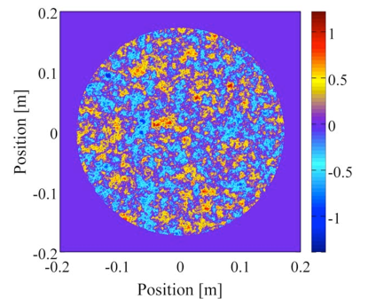
Figure 2: Surface figure (in nm) of a typical generated phase map with Piston, tilt, power and astigmatism terms subtracted.

III Degenerate Perturbation-Theory Analysis

III.1 Laugerre-Gauss modes

The Laguerre-Gauss modes (LG_p,l) are a set of circularly symmetric modes which can be written in cylindrical coordinates as Siegman

$$\begin{split}u_{p,l}(r,\phi,z)&=\sqrt{\frac{2\,p!}{\pi(|l|+p)!}}\frac{1}{\omega(z)}\left[\frac{\sqrt{2}r}{\omega(z)}\right]^{|l|}\\ &\times L_{p}^{|l|}\left[\frac{2r^{2}}{\omega^{2}(z)}\right]\exp[i(2p+|l|+1)\psi(z)]\\ &\times\exp\left[-ik\frac{r^{2}}{2R(z)}+il\phi\right]\exp\left[\frac{-r^{2}}{\omega^{2}(z)}\right],\end{split}$$ (3)

where $\omega(z)$ is the beam radius, $\psi(z)$ is the Gouy phase, and $R(z)$ is phase front curvature of the beam. $L_{p}^{|l|}(x)$ is the associated Laguerre polynomial where $p\geq 0$ and $l$ are the radial and azimuthal indices respectively.

The mode selectivity of the cavity is determined by the cavity finesse and the mode dependent phase shift $(2p+|l|+1)\psi(z)$. From this we see that the LG_p,l mode has $2p+|l|+1$ degenerate eigenmodes. For example, LG_3,3 belongs to a 10-fold degenerate space, which can be spanned by: LG_3,±3, LG_0,±9, LG_1,±7, LG_2,±5 and LG_4,±1.

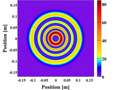
Figure 3: Normalized intensity distribution of the $\rm{LG}_{3,3}$ mode at the mirror position ($\omega_{0}=0.021$ m, $z=1997.25$ m).

Coating Brownian noise power is proportional to the integral of beam intensity, as the scaling law (Eq. (1)) indicates. In Table 2, we present theoretical thermal noise suppression factors for selected LG modes. To permit a fair comparison, the widths of all modes considered here and henceforth were chosen to be $0.018$ m, which yield a clipping loss Freise:LG , due to the finite size of the cavity mirrors, of around 1 ppm. We see that the LG_3,3, considered by many as the leading candidate for use in gravitational wave interferometers, offers a theoretical thermal noise reduction factor of $\sim$1.6 compared to a standard Gaussian beam (LG_0,0). The transverse intensity distribution of the LG_3,3 mode is presented in Fig. 3.

Table 2: Suppression factors of thermal noise (in power spectral density) for LG modes with a fixed clipping loss of 1 ppm.

		${\rm LG_{0,0}}$		${\rm LG_{0,9}}$		${\rm LG_{1,7}}$		${\rm LG_{2,5}}$		${\rm LG_{3,3}}$		${\rm LG_{4,1}}$
Beam radius
(mm)		$9.96$		16.5		17.3		17.9		18.2		18.4
Suppression
Factor		1		1.51		1.62		1.64		1.61		1.51

III.2 Application of Degenerate Perturbation Theory to the Perturbed Fabry-Perot Cavity

The combination of eigenmodes excited in a cavity depends on the composition of the incident field and on the properties of the cavity itself. In this section we discuss how first-order perturbation theory can be applied to this problem. We first explore how mirror figure error breaks the degeneracy of LG cavity modes before describing the phase shift each mode experiences in an optical cavity and finally constructing the total field (prompt plus leakage) reflected from a perturbed Fabry-Perot resonator.

III.2.1 Mode Splitting

Fig. 4 illustrates light propagation in a simple Fabry-Perot cavity, introducing the notation employed in our formalism.

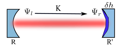
Figure 4: Fabry-Perot cavity with a perturbation $\delta h(x,y)$ on the end mirror.

We use the following standard method for propagating cavity fields,

$$\Psi_{r}(\vec{r})=\int K(\vec{r},\vec{r}\,^{\prime})\Psi_{l}(\vec{r}\,^{\prime})\,\mathrm{d}^{2}\vec{r}\,^{\prime},$$ (4)

or $|\Psi_{r}\rangle=\hat{K}|\Psi_{l}\rangle$, where $\Psi_{r}$ and $\Psi_{l}$ are the electric fields near the right and left mirror respectively and $K$ is the field propagator from the left mirror to the right

$$K(\vec{r},\vec{r}\,^{\prime})=\frac{ik}{2\pi L}e^{-\frac{ik}{2L}|\vec{r}-\vec{r}\,^{\prime}|^{2}}.$$ (5)

Therefore, if $|\psi\rangle$ is an eigenmode of the cavity,

$$|\psi\rangle=\hat{R}\hat{K}\hat{R}^{\prime}\hat{K}|\psi\rangle,$$ (6)

where $\hat{R}$ is the reflection operator of the left mirror and $\hat{R}^{\prime}$ is for the right. Hence, $|\psi\rangle$ is an eigenmode of the operator $(\hat{R}\hat{K}\hat{R}^{\prime}\hat{K})$.

We assume that the mirror on the left is ideal and study the consequences of applying a surface figure perturbation $\delta h$ to the right hand (end mirror) optic. The reflection operator $\hat{R}^{\prime}$ can then be written as

$$\hat{R^{\prime}}=\hat{R}e^{2ik\delta h}\approx\hat{R}(1+2ik\delta h).$$ (7)

To obtain the real cavity eigenmodes, we need to solve for the eigenfunctions of $(\hat{R}\hat{K}\hat{R}^{\prime}\hat{K})$. Note that the original LG₃₃ mode is an eigenfunction of an unperturbed cavity:

$$|33\rangle=(\hat{R}\hat{K}\hat{R}\hat{K})|33\rangle.$$ (8)

As introduced above, the LG₃₃ mode is degenerate with $9$ other modes, each having eigenfrequency $\omega_{0}$, thus $\hat{R}\hat{K}\hat{R}\hat{K}$ also has $10$ degenerate eigenmodes at $\omega_{0}$.

For reasonable parameters, modes outside of this degenerate sub-space are far enough from resonance that we may ignore them in this first-order analysis. Therefore, to good approximation, we can assume the new eigenmodes of the perturbed cavity are still members of the Hilbert space of the original $10$ LG modes, which we represent by $|i\rangle$, (i=1,2,…,10). These new eigenmodes, denoted $|i^{\prime}\rangle$, are the eigenvectors of the matrix with elements $\langle i|\hat{R}\hat{K}\delta h\hat{R}\hat{K}|j\rangle=\langle i|\delta h|j\rangle$, $(i,j=1,2,\ldots,10)$

$$\begin{pmatrix}\langle 1|\delta h|1\rangle&\ldots&\langle 1|\delta h|10\rangle\\ \vdots&\ddots&\vdots\\ \langle 10|\delta h|1\rangle&\ldots&\langle 10|\delta h|10\rangle\end{pmatrix}.$$ (9)

Denoting the electric field of $|i\rangle$ as $\phi_{i}$, we write

$$\langle i|\delta h|j\rangle=\int\int\phi^{*}_{i}(x,y)\delta h(x,y)\phi_{j}(x,y)\,\mathrm{d}x\,\mathrm{d}y.$$ (10)

The frequency shift of the degenerate modes introduced by the perturbation is then proportional to the eigenvalues of the matrix

$$\omega_{i}=\frac{kc}{L}\langle i^{\prime}|\delta h|i^{\prime}\rangle,$$ (11)

where $k=2\pi/\lambda$ is the optical wavenumber, $c$ is the speed of light and $L$ is the cavity length.

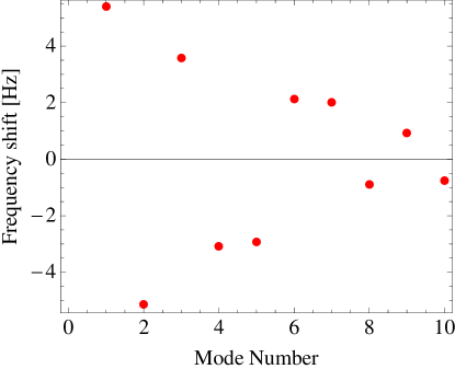
Figure 5: Frequency shift of LG modes introduced as a result of realistic mirror perturbations.

This quantity was evaluated using the reference map shown above (Fig. 2). The RMS roughness of the reference was scaled to be similar to those of measured Advanced LIGO mirror surfaces (0.3 nm RMS). Results are presented in Fig. 5. Here the frequency splits are given in Hertz ($\omega/2\pi$). The frequency shifts are one order of magnitude smaller than the advanced gravitational-wave interferometer’s cavity linewidth. Thus, multiple perturbed eigenmodes will be partially resonant, radically distorting the shape of the output field.

III.2.2 The Modal Input-Output Equation

Above we have shown that mirror figure errors will lift the modal degeneracy and split the degenerate LG_3,3 space into distinct states with unique eigenfrequencies. We now consider how each of these modes interacts with a cavity.

For any mode $|\rm in\rangle$ injected into an ideal cavity, there exists a frequency dependent phase shift between the input and total reflected or output fields. This can be written as Milburn

$$|{\rm out}\rangle=\frac{\gamma_{c}+i(\omega-\omega_{0})}{\gamma_{c}-i(\omega-\omega_{0})}|{\rm in}\rangle,$$ (12)

where $\omega$ is the frequency of the injected field, $\omega_{0}$ is the resonant frequency of the cavity closest to $\omega$ and $\gamma_{c}=c{\rm T_{\mathrm{input}}}/4L$ is the cavity pole frequency in Hertz. Here, ${\rm T_{\mathrm{input}}}$ denotes the power transmissivity of the cavity input mirror; the transmissivity of the end mirror is assumed to be zero.

Suppose that this ideal cavity hosts an $N$-fold degenerate space and that we inject an input mode $|\rm in\rangle$ which belongs to this space. If the $N$-fold degeneracy is broken by some mirror figure error, the new eigenmodes can be approximated by $|n\rangle$, $n=1,2,\ldots,N$, where each mode still belongs to the original sub-space, but has a new eigenfrequency $\omega_{n}$. As we shall see in Appendix A, this is justified as long as the cavity finesse is high enough and the eigenfrequencies of the non-degenerate modes are well-separated from this sub-space.

The output from the perturbed cavity can be obtained by projecting the input mode $|\rm{in}\rangle$ onto the new basis $|n\rangle$ and calculating the phase shifts using the following relation:

$$|{\rm out}\rangle=\sum_{n^{\prime}=1}^{N}\frac{\gamma_{c}+i(\omega-\omega_{n^{\prime}})}{\gamma_{c}-i(\omega-\omega_{n^{\prime}})}|n^{\prime}\rangle\langle n^{\prime}|{\rm in}\rangle.$$ (13)

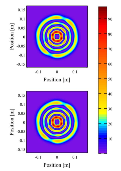
Figure 6: Intensity distributions of the total field reflected from an arm cavity whose end mirror was perturbed by the reference map. These distributions were calculated independently via two different techniques. Top – Analytic method described in Section III.2. Bottom – FFT-based numerical simulation (see Section IV.2).

This procedure was applied to the LG_3,3 degenerate space using the resonant frequencies of the previous section, $\omega_{n}$. With the reference phase map scaled to 0.3 nm RMS, the intensity profile of the resulting output mode is shown in Fig. 6.

IV Contrast Defect

In gravitational-wave interferometers, contrast defect is defined as the ratio of the minimum possible optical power at the anti-symmetric (dark) port to the power incident on the beamsplitter. This quantity can be expressed as

$$C=\frac{P_{\mathrm{AS}}}{P_{\mathrm{X}}+P_{\mathrm{Y}}},$$ (14)

where X and Y are labels for the two arm cavities, $P_{\Box}=\iint_{\mathbb{R}^{2}}(\Psi^{\mathrm{out}}_{\Box})^{*}\Psi^{\mathrm{out}}_{\Box}\,\mathrm{d}x\mathrm{d}y$ and $\Psi^{\mathrm{out}}_{\mathrm{AS}}=\Psi^{\mathrm{out}}_{\mathrm{X}}-\Psi^{\mathrm{out}}_{\mathrm{Y}}$ represents the field at the anti-symmetric port (AS) of the interferometer.

In principle, the dark port could be completely dark. However, the presence of intentional imbalances in the arms (finite beamsplitter size, Schnupp asymmetry, etc.) and unintentional imperfections (mirror shape, scatter loss, mirror motion, etc.) result in imperfect destructive interference between the fields which recombine at the beamsplitter. This imperfect interference leads to the leakage of some ‘junk’ light to the dark port where the gravitational-wave signal is also detected. Excess light at the dark port can lead to a degradation of sensitivity via several mechanisms and compromise the robust operation of interferometer longitudinal and alignment control systems Sigg:ReadoutControl ; Nic:Contrast . Contrast defect is thus a useful metric to employ when comparing interferometer configurations.

The above perturbation analysis shows that the fields resonating in the arm cavities of a real interferometer will no longer be pure LG_3,3 modes. Further, the relative amplitudes of the quasi-degenerate modes are strongly dependent on mirror properties, which will, in general, be different for each arm. Hence the perturbed arm cavity fields will interfere imperfectly at the beamsplitter. We therefore expect an LG_3,3 interferometer to exhibit a larger contrast defect than e.g. an LG_0,0 mode. We now test this hypothesis by analytical and numerical means.

IV.1 Analytic calculation

According to Appendix A, the contrast defect in an interferometer with one perfect arm cavity and one perturbed arm cavity, can be analytically written as

$$\epsilon=1-|\langle\rm{in}|\rm{out}\rangle|,$$ (15)

when the mirror perturbations are sufficiently small ($\epsilon\ll 1$).

Appendix A also shows that when a frequency shift is small compared with the line width of the cavity, i.e. $\omega-\omega_{n}\ll\gamma$, Eq. 15 can be approximated as

$$\epsilon=\left[\sum_{n^{\prime}}\langle 33|\delta h|n^{\prime}\rangle\langle n^{\prime}|\delta h|33\rangle-\langle 33|\delta h|33\rangle^{2}\right]\left(\frac{8\sqrt{2}\pi}{\lambda{\rm T}}\right)^{2},$$ (16)

where

$$\langle 33|\delta h|pl\rangle=\int\delta h(u_{33}^{*}u_{pl})\,\mathrm{d}x\,\mathrm{d}y.$$ (17)

Alternatively, this can be written as

$$\epsilon=\left[\frac{(8\sqrt{2}\pi)}{\lambda T}\right]^{2}\delta z^{2},$$ (18)

where

$$\delta z^{2}=\sum_{2p+|l|=10\atop(p,l)\neq(3,3)}|\langle 33|\delta h|pl\rangle|^{2}\,.$$ (19)

This suggests that in order to minimize contrast defect, one must strive to suppress the projection of $\delta h$ onto the 9 complex basis functions, given by $u_{33}^{*}u_{pl}$. Since these functions are complex and $\delta h$ is real, this actually corresponds to 18 basis functions.

Based on Eq. (13), the contrast defect has been evaluated analytically in the case that only the end mirror (ETM) of one cavity is perturbed with the reference phase map of Fig .2. The perturbation for different RMS values was obtained by rescaling the reference phase map. The results are shown in Fig. 7.

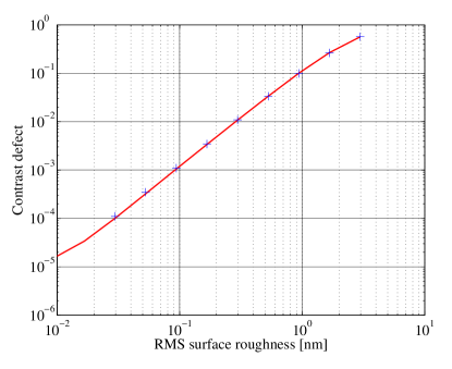
Figure 7: Contrast defect with the ETM of one cavity perturbed by rescaling the reference phase map: Solid red is from the analytical calculation, blue marker is from the FFT calculation.

One can show that, for small perturbations, perturbing two cavity mirrors using phase maps derived from the same power spectral density function, will, on average, result in twice the contrast defect when compared to perturbations of a single mirror. However, depending on the spatial correlations between the mirrors, the contrast defect can be as much as twice the average in some cases.

IV.2 Numerical calculation

To confirm the results obtained via perturbation theory and to extend our analysis to more complicated configurations, a parallel investigation was carried out using numerical methods. We utilized an FFT-based field propagation tool – the Stationary Interferometer Simulation (SIS) SIS .

SIS is predominantly used to inform the design of the Advanced LIGO interferometers and is under continuous development at Caltech’s LIGO Laboratory. SIS employs an iterative procedure to find the stationary fields for a given optical configuration and input beam. Mirror surface maps can be generated from user-defined power spectral density functions, allowing one to study the effects of various hypothetical mirror aberrations. Cavity systems are ‘locked’ using a Pound-Drever-Hall signal Drever to realize an operating condition similar to that which would be observed experimentally.

SIS was used to model Advanced LIGO Fabry-Perot arm cavities supporting LG_0,0, LG_3,3 and nearly-concentric mesa modes Bondarescu:Mesa ; Miller:Thesis . The parameters of the LG_3,3 and mesa cavities (see Table 3) were adjusted to yield systems with round-trip diffraction loss equivalent to that of the fiducial LG_0,0 resonator ($\lesssim 1$ ppm). In each case the input beam remained fixed as the beam which was ideally coupled to an unperturbed cavity. To suppress the aliasing effect, a larger FFT grid of 1024$\times$1024 points on a 0.7 m$\times$0.7 m square was used for all modes.

Table 3: Cavity parameters used in the numerical simulations. All three resonators had a length of 3994.5 m. The mesa radii of curvature refer to the fiducial sphere from which the mesa correction profile is subtracted (c.f. Bondarescu:Mesa ). Cavity g factor is not well defined for mesa modes.

	LG0,0	LG3,3	Mesa
Ritm	1934 m	2857 m	1997.25 m
Retm	2245 m	2857 m	1997.25 m
Cavity g factor	0.83	0.16	—

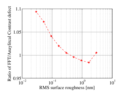
Figure 8: Ratio, numerical/analytical, of single-cavity contrast defects calculated with the end mirror perturbed by a 0.3 nm RMS figure error.

Initially SIS was used to simulate a configuration identical to that studied analytically. Under these conditions both sets of results are in good agreement (better than 10%) (see Figs. 6, 7 and 8). The flexibility of SIS was then used to consider more complex simulations where both cavity mirrors are perturbed and to emulate a Fabry-Perot Michelson interferometer. SIS was also employed to study high-RMS cases in which the analytic approximation breaks down.

For each simulation run, two random surfaces, with a specified RMS roughness and a spatial spectrum approximating that of the first Advanced LIGO mirrors (see Fig. 1), were generated and added to the profiles of the cavity mirrors. SIS then evaluated the field $\Psi^{\mathrm{out}}$ reflected from the cavity at its operating point, which is chosen from the cavity which is locked by using the Pound-Drever-Hall error signal.

Results from two discrete, single-cavity simulations, representing the $X$ and $Y$ arms of an interferometer, were then combined according to Eq. 14 to estimate interferometer contrast defect. Multiple trials were conducted at each value of RMS surface roughness with different random maps, allowing one to consider more than 100 unique arm cavity pairs. From these data, the mean and standard deviation of interferometer contrast defect were found as a function of mirror aberration RMS. Results for all three beams are shown in Fig. 9. The simulated contrast defect for Gaussian beam (TEM00) is consistent with the measured value of LIGO, which is around $10^{-4}$  LIGOcon and low enough for the effective detection.

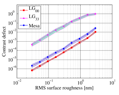
Figure 9: Interferometer contrast defect as a function of test mass surface roughness (all 4 mirrors are perturbed with random phase map at the same level of RMS). Solid markers report mean values of numerical results with the corresponding shaded regions illustrating one standard deviation (see IV.2), which is roughly four times higher than the trace in Fig. 7

Our numerical work confirms the result from perturbation theory; LG_3,3 interferometers are more sensitive to mirror surface roughness than those supporting a fundamental Gaussian mode. We further show that LG_3,3 beams are also outperformed in this respect by nearly-concentric mesa beams, indicating that this sensitivity arises due to the properties of the Laguerre-Gauss mode itself and is not an inevitable handicap for all beams capable of mitigating mirror thermal noise.

V Contrast Defect Improvement

Here we examine several methods of reducing the contrast defect.

V.1 Better polishing

The most direct approach is to reduce the mirror figure error. However, reaching appropriate levels of surface roughness is beyond the capabilities of current technology. We estimate that in order to achieve reasonable performance, LG_3,3 modes require mirrors with an RMS roughness roughly one order of magnitude smaller than is currently achievable (assuming the mirror coatings introduce no additional roughness, i.e. perfectly smooth, uniform coatings).

In the remainder of this section, we thus consider more unconventional means of reducing the contrast defect. Fig. 10 shows the results of each investigation.

Figure 10: Analytic calculation with different conditions for reducing the contrast defect: solid curve is the original contrast defect; dashed line has corrective rings added to the phase map; dotted curve is with detuned injecting laser frequency.

V.2 Arm cavity detuning

Equation (12) shows that the output field varies with the frequency of light injected into a cavity, or equivalently with cavity length. This motivated us to study the variation in contrast defect as a function of arm cavity detuning.

It was found that detuning was effective in modifying contrast defect. Unfortunately, the large detuning necessary to recover good contrast had the effect of simultaneously reducing the optical power circulating in the cavity.

With a detuning of 100 Hz (approximately two cavity linewidths), it was possible to recover acceptable contrast (dotted line, Fig. 10). However, the same detuning causes the circulating power to drop by $\sim$60%. We therefore do not consider this approach to be viable in gravitational-wave interferometers where the injected frequency is usually tuned to maximize the optical power circulating in the coupled-cavity system. This technique can, however, be considered for experiments where the thermal noise needs to be reduced, but the cavity’s stored power is not of concern.

V.3 Mirror Corrections

The increase in contrast defect observed when using LG_3,3 modes in the presence of realistic surface roughness results from the presence of multiple pseudo-degenerate higher order modes. Here we attempt to see if this effect can be mitigated by depositing corrective structures on the mirror’s surface.

By introducing material at the nodes of the desired LG_3,3 mode it was hoped that the unwanted modes from the same sub-space could be suppressed.

As a concrete example, two Gaussian rings were added to the random phase map at nodes 1 and 3 of the LG_3,3 mode. Each ring was of the form:

$$f(x,y)=\frac{\lambda}{20}e^{-\frac{(r-r_{p})^{2}}{2(R/100)^{2}}}.$$ (20)

where $r_{p}$ indicates the position of the different nodes. The frequency split is plotted in Fig. 11. Compared to Fig. 5, the frequency splits under this condition are much larger, therefore the other degenerate modes will be harder to excite.

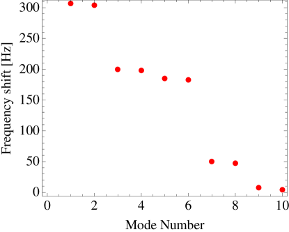
Figure 11: Frequency shift in LG modes introduced by adding rings to the reference phase map.

The analytically computed contrast defect for this case is plotted as the dashed line in Fig. 10. Although the defect is improved for values of surface roughness similar to that which is currently achievable, we find that, in order to significantly break the modal degeneracy, the height of the rings must be increased to such a degree that the induced scatter becomes unacceptably high ($\sim$ 500 ppm), reducing the stored power and thus the interferometer’s phase sensitivity. We hence conclude that this approach is not promising.

At Caltech, Yamamoto has studied a similar approach whereby the mirror reflectivity is set to zero at the nodes of the LG_3,3 mode HiroNote . This technique was found to be similarly unsuitable for application to gravitational wave interferometers.

V.4 Mode Healing

Previous work Brett:DR has shown that the presence of a signal recycling cavity can substantially reduce the contrast defect in the case where the resonant mode in the interferometer is TEM_0,0. The higher order transverse modes are not resonant in the signal recycling cavity and are therefore suppressed. In the LG_3,3 case, however, the signal cavity is resonant for the LG_3,3 mode as well as all of the modes which are in the degenerate sub-space. Therefore, our expectation is that there would not be a mode healing effect when using any higher order mode which can be split in this way. In the case where the signal recycling cavity is detuned to amplify the gravitational wave response at a particular frequency, the situation could be significantly more complicated due to the frequency splitting shown in Fig. 5. To quantitatively explore the effect of the compound cavity on degenerate modes, further analytic and numerical work is required.

VI Conclusions

In this paper, we use numerical analysis as well as perturbation theory to analyze the modes of a Fabry-Perot cavity resonating a LG_3,3 beam. We prove that with realistic mirror figure errors, the real output mode of the cavity will change significantly, resulting in an unacceptable increase of the contrast defect.

We also investigate unconventional corrective techniques to reduce the contrast defect. While they turn out to be unsuitable for quantum shot noise limited interferometers, they may have some utility for other classes of cavities. For LG_3,3 modes to function effectively, we estimate that surface figure errors must be reduced to the order of $10^{-2}$ nm RMS to achieve the required contrast defect of LIGO($\sim 10^{-4}$). Such precise polishing and coating uniformity will likely not be available for several years. Using high-order Laguerre-Gauss modes in standard spherical mirror cavities appears to be a poor choice in light of current technologies.

Numerical simulations using mesa and normal Gaussian beams show these beams are not so sensitive to figure errors. Future effort will be directed toward the construction of a new family of optical modes which can reduce the thermal noise impact while simultaneously being robust against mirror imperfections.

VII Acknowledgements

We thank Andreas Freise, Matteo Barsuglia, and Bill Kells for several illuminating discussions. Many thanks to Eric Gustafson and Huan Yang for a careful reading of this manuscript. TH and YC are supported by NSF Grant PHY-0601459, PHY-0653653, CAREER Grant PHY-0956189, and the David and Barbara Groce Startup Fund at the California Institute of Technology. RA and HY are supported by the National Science Foundation under grant PHY-0555406. JM is the recipient of an Australian Research Council Post Doctoral Fellowship (DP110103472).

Appendix A Contrast Defect

Here we show that the contrast defects defined in equations (15) and (14) are equivalent in the limit of small perturbations. We denote the input and output field for the two cavities (X and Y) as $|{\rm in}\rangle_{X},|{\rm out}\rangle_{X},|{\rm in}\rangle_{Y},|{\rm out}\rangle_{Y}$. In our analytical calculation, we assume the input and output fields of each cavity are normalized, because we ignore transmissivity of the ETM, and the diffraction loss, so that we have

$$\langle{\rm in}|{\rm in}\rangle_{X}=\langle{\rm in}|{\rm in}\rangle_{Y}=\langle{\rm out}|{\rm out}\rangle_{X}=\langle{\rm out}|{\rm out}\rangle_{Y}=1.$$ (21)

We can then write

$$P_{X}=\langle{\rm in}|{\rm in}\rangle_{X}=1,P_{Y}=\langle{\rm in}|{\rm in}\rangle_{Y}=1$$ (22)

and the power at the anti-symmetric port can be written as

$$P_{AS} = \||{\rm out}\rangle_{X}-|{\rm out}\rangle_{Y}\|^{2}$$ (23)

$$= 2-\langle{\rm out}|{\rm out}\rangle_{XY}-\langle{\rm out}|{\rm out}\rangle_{YX}.$$

With the definition of contrast defect in Eq. (15), we have

$$\epsilon_{X}=1-|\langle{\rm in}|{\rm out}\rangle_{X}|,\epsilon_{Y}=1-|\langle{\rm in}|{\rm out}\rangle_{Y}|$$ (24)

so that we can write the output field as

$$|{\rm out}\rangle_{X}=(1-\epsilon_{X})e^{i\phi_{X}}|\rm in\rangle_{X}+|\delta_{X}\rangle$$

$$|{\rm out}\rangle_{Y}=(1-\epsilon_{Y})e^{i\phi_{Y}}|\rm in\rangle_{Y}+|\delta_{Y}\rangle$$ (25)

where

$$\langle\delta_{X}|{\rm in}\rangle_{X}=0,\langle\delta_{X}|\delta_{X}\rangle=\epsilon_{X}$$

$$\langle\delta_{Y}|{\rm in}\rangle_{Y}=0,\langle\delta_{Y}|\delta_{Y}\rangle=\epsilon_{Y}$$

$$\langle\delta_{X}|{\rm in}\rangle_{Y}=\langle\delta_{Y}|{\rm in}\rangle_{X}=0$$ (26)

In both the analytical and numerical calculations, we assume one of the two interferometer cavities is perfect and the other is with mirror figure errors, so here we can write $\epsilon_{Y}=1,|\delta_{Y}\rangle=0$, therefore, to the first order approximation ($\epsilon_{X}\ll 1$), we get obtain

$$P_{AS}=2\epsilon_{X}$$ (27)

which shows that the contrast defect defined in Eq. (14) is the same as the analytical definition in Eq. (15).

When we consider two cavities both with imperfections, if they are statistically independent, we can write $\langle\delta_{X}|\delta_{Y}\rangle=0$, so that the average value of the contrast defect of the system is

$$P_{AS}=2(\epsilon_{X}+\epsilon_{Y}).$$ (28)

We now show that Eq. (15) can be approximately written as given in Eq. (16). From Eq. (13), we have

$$\langle{\rm in}|{\rm out}\rangle=\sum_{n^{\prime}}\frac{\gamma+i(\omega-{\omega_{n}^{\prime}})}{\gamma-i(\omega-\omega_{n^{\prime}})}\langle{\rm in}|n^{\prime}\rangle\langle n^{\prime}|{\rm in}\rangle$$ (29)

when $\omega-\omega_{n^{\prime}}\ll\gamma$, Eq. (29) can be expanded as

$$\sum_{n^{\prime}}\left[1+\frac{2i(\omega-\omega_{n^{\prime}})}{\gamma}-\frac{2(\omega-\omega_{n^{\prime}})^{2}}{\gamma^{2}}\right]\langle{\rm in}|n^{\prime}\rangle\langle n^{\prime}|{\rm in}\rangle$$ (30)

Note that when the mode frequency is shifted $\omega_{n^{\prime}}$, the optical power in the cavity is maximized, so that the linear term vanishes, therefore that the modulated frequency of the beam $\omega$ can be given by:

$$\omega=\frac{kc}{L}\langle 33|\delta h|33\rangle$$ (31)

The contrast defect defined in Eq. (15) is

$$\epsilon = \sum_{n^{\prime}}\frac{2(\omega-\omega_{n^{\prime}})^{2}}{\gamma^{2}}\langle{\rm in}|n^{\prime}\rangle\langle n^{\prime}|{\rm in}\rangle$$ (32)

$$= \frac{2}{\gamma^{2}}\left(\sum_{n^{\prime}}\langle{\rm in}|n^{\prime}\rangle\omega_{n^{\prime}}^{2}\langle n^{\prime}|{\rm in}\rangle-\omega^{2}\right)$$

After perturbation, the frequency split is the eigenvalue of the matrix given in Eq. (9) and the eigenvector of the matrix is the real eigenmode of the cavity, thus we can write

$$\sum_{n^{\prime}}\langle{\rm in}|n^{\prime}\rangle\omega_{n^{\prime}}^{2}\langle n^{\prime}|{\rm in}\rangle$$

$$=\left(\frac{2\pi c}{\lambda{\rm L}}\right)^{2}\sum_{n^{\prime}m^{\prime}l^{\prime}}\langle{\rm in}|n^{\prime}\rangle\langle n^{\prime}|\delta h|m^{\prime}\rangle\langle m^{\prime}|\delta h|l^{\prime}\rangle\langle l^{\prime}|{\rm in}\rangle$$

$$=\left(\frac{2\pi c}{\lambda{\rm L}}\right)^{2}\sum_{m^{\prime}}\langle{\rm in}|\delta h|m^{\prime}\rangle\langle m^{\prime}|\delta h|{\rm in}\rangle$$ (33)

where $\gamma=c{T}/4{\rm L}$. Then, in this limit, when the injected field is $|33\rangle$, the contrast defect can be written as in Eq. (16).

References

- (1) LIGO Scientific Collaboration, “LIGO: The Laser Interferometer Gravitational-wave Observatory”, Reports on Progress in Physics (2009).
- (2) http://www.virgo.infn.it/.
- (3) http://www.geo600.de/.
- (4) http://tamago.mtk.nao.ac.jp/.
- (5) G. Harry, H. Armandula, E. Black, D. Crooks, G. Cagnoli, J. Hough, P. Murray, S. Reid, S. Rowan, P. Sneddon, M. Fejer, R. Route, and S. Penn, Appl. Opt. 45, 1569-1574 (2006).
- (6) R. F. Greene and H. B. Callen, Phys. Rev. D, 88, 6 (1952).
- (7) Y. Levin, Phys. Rev. D, 57, 659(1998).
- (8) G. Lovelace, Class. Quant. Gravity 24, 4491 (2007).
- (9) E. D’Ambrosio, R. OÕShaugnessy, K. Thorne, S. Strigin, and S. Vyatchanin, Class. Quant. Gravity 21, S867 (2004).
- (10) B. Mours, E. Tournefier, and J.-Y. Vinet, Class. Quant. Gravity 23, 5777 (2006).
- (11) M. Bondarescu and K. S. Thorne, Phys. Rev. D, 74, 082003 (2006).
- (12) J. Miller, PhD. Thesis, U. of Glasgow (2010).
- (13) M. Bondarescu, O. Kogan, and Y. Chen, Phys. Rev. D 78, 082002 (2008).
- (14) M. Granata and C. Buy and R. Ward and M. Barsuglia, Phys. Rev. Lett. 105, 231102(2010).
- (15) P. Fulda, K. Kokeyama, S. Chelkowski, and A. Freise, Phys. Rev. D, 82, 012002 (2010).
- (16) This algorithm is based on techniques developed by F. Bondu (Observatoire de la Côte d’Azur/ Institut de Physique de Rennes).
- (17) A. E. Siegman, Lasers, University Science Books (1986).
- (18) S. Chelkowski, S. Hild and A. Freise, Phys. Rev. D 79, 122002 (2009)
- (19) G. J. Milburn, Quantum Optics, Springer-Verlag (1994)
- (20) P. Fritschel, R. Bork, G. González, N. Mavalvala, D. Ouimette, H. Rong, D. Sigg, and M. E. Zucker, Appl. Optics 40, 4988(2001).
- (21) N. Smith-Lefebvre, S. Ballmer, M. Evans, S. Waldman, K. Kawabe, V. Frolov, N. Mavalvala, LIGO Document, P1100025-v8 (2011)
- (22) Polish and Metrology from Tinsley Optics http://www.asphere.com, LIGO Technical Document G1100216 (2011)
- (23) H. Yamamoto, “SIS (Stationary Interferometer Simulation) manual”, LIGO Technical Document, T070039-v3 (2010).
- (24) R. W. P. Drever et al., App. Phys. B 31, 97-105 (1983).
- (25) S. W. Ballmer, Ph.D. thesis, MIT(2006).
- (26) H. Yamamoto, LIGO Technical note T1100220-v1 (2011).
- (27) B. Bochner, General Rel. and Grav. 35 (2003)