The Origins of AGN Obscuration: The ‘Torus’ as a Dynamical, Unstable Driver of Accretion

Abstract

Recent multi-scale simulations have made it possible to follow gas inflows responsible for high-Eddington ratio accretion onto massive black holes (BHs) from galactic scales to the BH accretion disk. When sufficient gas is driven towards a BH, gravitational instabilities generically form lopsided, eccentric disks that propagate inwards from larger radii. The lopsided stellar disk exerts a strong torque on the gas, driving inflows that fuel the growth of the BH. Here, we investigate the possibility that the same disk, in its gas-rich phase, is the putative “torus” invoked to explain obscured active galactic nuclei and the cosmic X-ray background. The disk is generically thick and has characteristic $\sim 1-10\,$pc sizes and masses resembling those required of the torus. Interestingly, the scale heights and obscured fractions of the predicted torii are substantial even in the absence of strong stellar feedback providing the vertical support. Rather, they can be maintained by strong bending modes and warps/twists excited by the inflow-generating instabilities. A number of other observed properties commonly attributed to “feedback” processes may in fact be explained entirely by dynamical, gravitational effects: the lack of alignment between torus and host galaxy, correlations between local SFR and turbulent gas velocities, and the dependence of obscured fractions on AGN luminosity or SFR. We compare the predicted torus properties with observations of gas surface density profiles, kinematics, scale heights, and SFR densities in AGN nuclei, and find that they are consistent in all cases. We argue that it is not possible to reproduce these observations and the observed column density distribution without a clumpy gas distribution, but allowing for simple clumping on small scales the predicted column density distribution is in good agreement with observations from $N_{\rm H}\sim 10^{20}-10^{27}\,{\rm cm^{-2}}$. We examine how the $N_{\rm H}$ distribution scales with galaxy and AGN properties. The dependence is generally simple, but AGN feedback may be necessary to explain certain trends in obscured fraction with luminosity and/or redshift. In our paradigm, the torus is not merely a bystander or passive fuel source for accretion, but is itself the mechanism driving accretion. Its generic properties are not coincidence, but requirements for efficient accretion.

1 Introduction

It has long been realized that bright, high-Eddington ratio accretion (i.e., a quasar) dominates the accumulation of mass in the supermassive BH population (Soltan, 1982; Salucci et al., 1999; Shankar et al., 2004; Hopkins et al., 2006d). The discovery, in the past decade, of tight correlations between black hole mass and host spheroid properties including mass (Kormendy & Richstone, 1995; Magorrian et al., 1998), velocity dispersion (Ferrarese & Merritt, 2000; Gebhardt et al., 2000), and binding energy or potential well depth (Hopkins et al., 2007b, a; Aller & Richstone, 2007; Feoli & Mancini, 2009) implies that black hole (BH) growth is tightly coupled to the process of galaxy and bulge formation. Increasingly, models invoke feedback processes from active galactic nuclei (AGN) to explain a host of phenomena, from the origin of the $M_{\rm BH}-\sigma$ relation, to rapid quenching of star formation in bulges, to the buildup of the color-magnitude relation and resolution of the cooling flow problem (see e.g. Silk & Rees, 1998; Di Matteo et al., 2005; Springel et al., 2005a; Hopkins et al., 2008a; Hopkins & Elvis, 2010; Croton et al., 2006; Cattaneo et al., 2009, and references therein).

Observations have demonstrated that most of the accretion luminosity in the Universe is obscured by large columns of gas and dust (e.g. Lawrence, 1991; Risaliti et al., 1999; Hill et al., 1996; Simpson et al., 1999; Willott et al., 2000; Simpson & Rawlings, 2000; Hao et al., 2005; Ueda et al., 2003, and references therein). This obscured AGN population dominates the population of X-ray sources (Miyaji et al., 2001; Ueda et al., 2003; Nandra et al., 2005; Hasinger et al., 2005; Steffen et al., 2003; Grimes et al., 2004; Hasinger, 2004; Sazonov & Revnivtsev, 2004; Barger & Cowie, 2005; Gilli et al., 2007; Hasinger, 2008), and accounts for most of the observed X-ray background luminosity (Setti & Woltjer, 1989; Madau et al., 1994; Comastri et al., 1995; Treister & Urry, 2006; Gilli et al., 2007). It may dominate the bright end of the infrared luminosity function as well (Sanders & Mirabel, 1996; Komossa et al., 2003; Ptak et al., 2003; Hickox et al., 2007; Daddi et al., 2007; Alexander et al., 2008; Hopkins & Hernquist, 2010). The abundance of obscured quasars remains a major uncertainty in reconciling synthesis models of AGN populations with the BH mass function today, and (by implication) understanding the radiative efficiencies of quasars (Salucci et al., 1999; Yu & Tremaine, 2002; Hopkins et al., 2007c; Shankar et al., 2009). Various specific galaxy populations (for example EXOs, XBONGs, ULIRGs, SMGs) commonly host obscured AGN (Yuan & Narayan, 2004; Georgantopoulos & Georgakakis, 2005; Max et al., 2005; Mainieri et al., 2005; Alexander et al., 2005; Daddi et al., 2007; Alexander et al., 2008; Riechers et al., 2008; Trump et al., 2009; Georgakakis et al., 2009; Nardini et al., 2009). And theoretical models have long predicted that in violent events such as galaxy mergers, there should be a transition from an early, “buried” accretion stage corresponding to e.g. “warm” ULIRGs and similar galaxies, to an at least partially un-obscured phase in which the AGN removes dust and gas and is visible as a bright quasar (Sanders et al., 1988a, b; King, 2003; Di Matteo et al., 2005; Hopkins et al., 2006a, c, b, 2008b, e, 2010; Hopkins & Hernquist, 2010; Younger et al., 2009).

Yet AGN obscuration remains poorly understood. The most popular models invoke a torus-shaped “donut” of obscuring material, on scales anywhere from $\sim 0.1-100\,$pc, to explain most of the heavily obscured AGN population (Antonucci, 1993; Lawrence, 1991). If one empirically assumes unification of obscured and unobscured AGN, then a number of the properties of the torus can be inferred: scale radii somewhere in the range above, and scale heights $h/R$ of order $\sim 1/3$ (Risaliti et al., 1999). The observed distributions of quasar and AGN column densities, and their detailed SED properties, place strong constraints on the densities, structure, and column densities within the obscuring material, with typical column densities as high as $\sim 10^{26}\,{\rm cm^{-2}}$ through the edge-on plane of the material. And direct observations are beginning to probe these scales, through combinations of diverse techniques such as adaptive optics and maser observations (Greenhill et al., 2003; Jaffe et al., 2004; Mason et al., 2006; Sánchez et al., 2006; Davies et al., 2006; Krips et al., 2007; Davies et al., 2007; Hicks et al., 2009; Ramos Almeida et al., 2009), giving constraints on the kinematics, gas and dynamical masses, and star formation rates at these scales. Indeed, this simple model of obscuration has proven successful at explaining a large number of AGN observables, and the torus forms the basis of most models uniting Type 1 and Type 2 AGN.

These successes should not mask the fact that the torus remains a phenomenological model. The simple “donut” picture is just a toy model – there are a large and growing number of un-ambiguous cases where it fails, whether in predicting detailed radiative transfer properties coming from the microphysical gas structure (Mason et al., 2006; Elitzur & Shlosman, 2006; Mor et al., 2009), or where the implied torus properties would involve bizarre radii and/or dust temperatures (Kuraszkiewicz et al., 2000; Tran, 2003; Page et al., 2004; Stevens et al., 2005; Ramos Almeida et al., 2009), or where it is simply clear that the dominant obscuration is isotropic, or time dependent, or comes from much larger scales (e.g. those associated with circumnuclear starbursts and/or the host galaxy; see Soifer et al., 1984; Scoville et al., 1986; Sanders et al., 1988a, b; Zakamska et al., 2006; Liu et al., 2009; Donley et al., 2005; Rigby et al., 2006; Schartmann et al., 2005; Hatziminaoglou et al., 2009; Rowan-Robinson et al., 2009; Martinez-Sansigre et al., 2009; Lagos et al., 2011).

Without a physical model for the origin and evolution of nuclear gas inflows, a large number of questions remain unanswered. Where do toroidal-like obscuring gas structures come from, in the first place? What determines their characteristic gas masses, radii, and structure? Why are such structures ubiquitous around AGN? Are they, in fact? It is also usually assumed that the torus is simply an obscuring “bystander” to the accretion event, or at most a passive fuel reservoir. But could the torus play some more critical role in the accretion process itself? A major long-standing puzzle is what drives and maintains the scale height of the torus – simple thermal pressure would be lost to cooling in a time much shorter than the local dynamical time. A large number of torus properties have been attributed to feedback from either young stars or the BH accretion itself – including the typical scale heights, clumping/phase structure, gaseous velocity dispersions, possible correlations between these quantities and star formation, and even the fueling rates onto the BH (e.g. Wada & Norman, 2002; Schartmann et al., 2009, and references therein). But it is important to recall that we do not yet understand the basic dynamics of gas and stars entirely in the absence of feedback!

There have been some attempts to address these from a physically motivated perspective, both in analytic and numerical work (Kawakatu & Wada, 2008; Cattaneo et al., 2005; Elvis, 2000; Hopkins & Elvis, 2010; Elitzur & Shlosman, 2006; Wada et al., 2009). However, analytic models are severely limited by the fact that the systems at these radii are highly non-linear, often chaotic, and not necessarily in steady state (with inflow, mass buildup, star formation, and feedback processes all competing). If one wishes to simultaneously follow the torus itself and the chaotic, non-symmetric gas inflows that form it in the first place, simulations are necessary. But simulations of galactic scales used to follow inflows and AGN obscuration have resolution of $\sim 100\,$pc, much larger than the relevant scales here (Cattaneo et al., 2005; Hopkins et al., 2005a, b).

Although progress has been made with zoom-in refinement techniques (see e.g. Escala, 2007; Levine et al., 2008; Mayer et al., 2007), the computational expense involved means that these simulations have, thus far, only barely probed that scales of interest and, in doing so, have made restrictive assumptions (typically explicitly turning off cooling and/or star formation on small scales); moreover they provide only a snapshot at one instant from the parent simulation – they cannot survey statistical properties of the nuclear region. Alternatively some simulations have simply adopted an assumed small-scale structure as an initial condition and studied the resulting gas dynamics at small radii (e.g. Schartmann et al., 2009; Wada & Norman, 2002; Wada et al., 2009). A number of important conclusions have been drawn from these studies; however, they not only bypass the question of the obscuring material origin, but also have thus far adopted idealized potentials, without live star formation and/or self-gravity of the gas. As such, the appearance and evolution of gravitational modes is suppressed. Cuadra et al. (2009) and Fukuda et al. (2000) show (albeit in similar idealized studies that neglected star formation and stellar feedback) that when included, gravitational torques from self-gravity are an order-of-magnitude stronger than hydrodynamic torques from pressure forces or viscosity; the same conclusions have been reached for intermediate ($\gtrsim 100\,$pc-scale) bars in a large number of hydrodynamic simulations (Noguchi, 1987, 1988; Hernquist, 1989; Barnes & Hernquist, 1991, 1996; Hopkins et al., 2009a), and follow from analytic arguments (see references above and Rice et al., 2005; Hopkins & Quataert, 2011a).

Recently, to understand the angular momentum transport required for massive BH growth, we have carried out a series of numerical simulations of inflow from galactic to BH scales (Hopkins & Quataert, 2010a). By re-simulating the central regions of galaxies, gas flows can be followed from galactic scales of $\sim 100\,$kpc to much smaller radii, with an ultimate spatial resolution $<0.1\,$pc. For sufficiently gas-rich disky systems, gas inflow continues all the way to $\lesssim 0.1$ pc. Near the radius of influence of the BH, the systems become unstable to the formation of lopsided, eccentric gas+stellar disks. This eccentric pattern is the dominant mechanism of angular momentum transport at $\lesssim 10$ pc, and can lead to accretion rates as high as $\sim 10\,M_{\sun}\,{\rm yr^{-1}}$, sufficient to fuel the most luminous quasars. In addition, through this process, some of the gas continuously turns into stars and builds up a nuclear stellar disk. Relics of these stellar disks may be evident around BHs in nearby galaxies (Hopkins & Quataert, 2010b), such as M31 and NGC4486b (Lauer et al., 1993; Tremaine, 1995; Bender et al., 2005; Lauer et al., 1996, 2005; Houghton et al., 2006; Thatte et al., 2000; Debattista et al., 2006). In this paper, we examine the possibility that the disk that drives accretion and accounts for these stellar relics, in its gas-rich phase, may in fact be the canonical torus-like obscuration region near AGN. If correct, this implies both an a priori understanding of torus formation and structure, and an entirely new paradigm in which to view the nature of AGN obscuration.

Specifically, we here perform a first comparison of these hydrodynamic simulations with the observed properties of AGN obscuration. We focus on dynamical properties and quantities such as the column density distribution that can be robustly predicted without reference to higher-order radiative transfer effects (which will be investigated in future work). In § 2, we summarize the properties of the numerical simulations, and in § 3 show how they naturally form torus-like obscuring structures. In § 4, we consider the scale heights and vertical structure of these torii, and examine how this can arise independent of stellar feedback from various gravitational processes. In § 5, we compare a number of observable dynamical properties of the predicted torii to nuclear-scale observations of AGN. We then in § 6 consider the full column density distribution, and in particular how it depends on sub-grid assumptions about the clumpiness of the ISM phase structure on un-resolved scales. We use this in § 7 to consider the predicted obscured fractions as a function of AGN and galaxy properties. Finally, we summarize our conclusions and discuss observational tests and future work in § 8.

2 The Simulations

The simulations described here are from a survey of multi-scale “zoom-in” runs which model gas inflows and star formation from large galactic scales to sub-pc scales, and have been discussed in a series of papers (Hopkins & Quataert, 2010a; Hopkins & Quataert, 2011a; Hopkins & Quataert, 2010b; Hopkins, 2010; Hopkins & Quataert, 2011b). A detailed description and list of simulations is presented in Hopkins & Quataert (2010a); we briefly summarize the salient properties here.

The simulations were performed with the TreeSPH code GADGET-3 (Springel, 2005); the detailed numerical methods are described there and in Springel & Hernquist (2002); Springel et al. (2005b). The simulations include collisionless stellar disks and bulges, dark matter halos, gas, and BHs. For this study, we are interested in isolating the physics of gas inflow. As a result, we do not include explicit models for BH accretion feedback – the BH’s only dynamical role is via its gravitational influence on scales $\lesssim 10\,$pc.

Because of the large dynamic range in both space and time needed for the self-consistent simulation of galactic inflows and nuclear disk formation, we use a “zoom-in” re-simulation approach. This begins with a large suite of simulations of galaxy-galaxy mergers, and isolated bar-(un)stable disks. These simulations have $0.5\times 10^{6}$ particles, corresponding to a spatial resolution of $50\,$pc. These simulations have been described in a series of previous papers (Di Matteo et al., 2005; Robertson et al., 2006c, b, a; Cox et al., 2006; Younger et al., 2008; Hopkins et al., 2009a). From this library of simulations, we select representative simulations of gas-rich major mergers of Milky-Way mass galaxies (baryonic mass $10^{11}\,M_{\sun}$), and their isolated but bar-unstable analogues, to provide the basis for our re-simulations. The dynamics on smaller scales does not depend critically on the details of the larger-scale dynamics. Rather, the small-scale dynamics depends primarily on global parameters of the system, such as the total gas mass channeled to the center relative to the pre-existing bulge mass.

Following gas down to the BH accretion disk requires much higher spatial resolution than is present in the galaxy-scale simulations. We begin by selecting snapshots from the galaxy-scale simulations at key epochs. In each, we isolate the central $0.1-1$ kpc region, which contains most of the gas that has been driven in from large scales. Typically this is about $10^{10}\,M_{\sun}$ of gas, concentrated in a roughly exponential profile with a scale length of $\sim 0.3-0.5\,$kpc. From this mass distribution, we then re-populate the gas in the central regions at much higher resolution, and simulate the dynamics for several local dynamical times. These simulations involve $10^{6}$ particles, with a resolution of a few pc and particle masses of $\approx 10^{4}\,M_{\sun}$. We have run $\sim 50$ such re-simulations, corresponding to variations in the global system properties, the model of star formation and feedback, and the exact time in the larger-scale dynamics at which the re-simulation occurs. Hopkins & Quataert (2010a) present a number of tests of this re-simulation approach and show that it is reasonably robust for this problem. This is largely because, for gas-rich disky systems, the central $\sim 300$ pc becomes strongly self-gravitating, generating instabilities that dominate the subsequent dynamics.

These initial re-simulations capture the dynamics down to $\sim 10$ pc, still insufficient to quantitatively describe accretion onto a central BH. We thus repeat our re-simulation process once more, using the central $\sim 10-30\,$pc of the first re-simulations to initialize a new set of even smaller-scale simulations. These typically have $\sim 10^{6}-10^{7}$ particles, a spatial resolution of $0.1\,$pc, and a particle mass $\approx 100\,M_{\sun}$. We carried out $\sim 50$ such simulations to test the robustness of our conclusions and survey the parameter space of galaxy properties. These final re-simulations are evolved for $\sim 10^{7}$ years – many dynamical times at $0.1$ pc, but short relative to the dynamical times of the larger-scale parent simulations. We also carried out a few extremely high-resolution intermediate-scale simulations, which include $\sim 5\times 10^{7}$ particles and resolve structure from $\sim$ kpc to $\sim 0.3\,$pc – these are slightly less high-resolution than the net effect of our two zoom-ins, but they obviate the need for a second zoom-in iteration and “bridge” the scales of the above simulation suites. The conclusions from these higher resolution simulations are identical.

Our simulations include gas cooling and star formation, with gas forming stars at a rate motivated by the observed Kennicutt (1998) relation. Specifically, we use a star formation rate per unit volume $\dot{\rho}_{\ast}\propto\rho^{3/2}$ with the normalization chosen so that a Milky-way like galaxy has a total star formation rate of about $1\,M_{\sun}\,{\rm yr^{-1}}$. Varying the exact slope or normalization of this relation has no qualitative effect on our conclusions. However, we caution that since we do not resolve the scales of individual bound star-forming cores in these simulations, the star formation is probably more uniform over the small radii than it would be in a more realistic ISM model. This is unlikely to be important for global properties here, but may have important consequences for e.g. detailed radiative transfer effects.

Because we cannot resolve the detailed processes of supernovae explosions, stellar winds, and radiative feedback, the effect of feedback from stars is crudely modeled with an effective equation of state (Springel & Hernquist, 2003). In this approach, feedback is assumed to generate a non-thermal (turbulent, in reality) sound speed that depends on the local star formation rate, and thus the gas density. Hopkins & Quataert (2010a) describe in detail the effects of different subgrid ISM sound speeds on angular momentum transport and inflow rates, and argue that observations favor effective turbulent speeds of $\sim 10-50\ {\rm km\,s^{-1}}$ for densities $\sim 1-10^{5}$ cm^-3, respectively. But because the real physics and their effects are uncertain, it is important to vary this prescription and determine which of our conclusions are sensitive to the assumed sub-grid properties.

Within the context of this model, we can interpolate between two extremes using a parameter $q_{\rm eos}$. At one end, the gas has an effective sound speed of $10\,{\rm km\,s^{-1}}$, motivated by, e.g., the observed turbulent velocity in atomic gas in nearby spirals or the sound speed of low density photo-ionized gas; this is the “no-feedback” case with $q_{\rm eos}=0$. This is broadly similar to what is assumed in Bournaud et al. (2007); Teyssier et al. (2010). The opposite extreme, $q_{\rm eos}=1$, represents the “maximal feedback” model of Springel et al. (2005b); in this case, $100\%$ of the energy from supernovae is assumed to stir up the ISM. This equation of state is substantially stiffer, with effective sound speeds as high as $\sim 200\,{\rm km\,s^{-1}}$. This is qualitatively similar to the near-adiabatic equations-of-state in the BH accretion studies of Mayer et al. (2007); Dotti et al. (2009). The sound speed at scales we consider cannot meaningfully be much larger than this, since it is similar to the circular/escape velocity. By varying $q_{\rm eos}$, we examine a spectrum of intermediate cases: for example, equations of state similar to the “starburst” model in Klessen et al. (2007) or the sub-GMC equation of state in Spaans & Silk (2005). Most of our suite of simulations focuses on a wide range of sub-grid sound speeds $\sim 20-100\,{\rm km\,s^{-1}}$, motivated by a variety of observations of dense, star forming regions both locally and at high redshift (Downes & Solomon, 1998; Bryant & Scoville, 1999; Förster Schreiber et al., 2006; Iono et al., 2007), and recent numerical simulations (Hopkins et al., 2011a).

Within this range, we found little difference in the physics of angular momentum transport or in the resulting accretion rates, gas masses, etc. on the scales we consider (Hopkins & Quataert, 2010a). More detailed comparison with the explicit stellar feedback models presented in Hopkins et al. (2011a, c, b) will be the subject of future work. Here, we will focus on the effects on the obscuring gas near the BH. Because we are not explicitly accounting for or resolving feedback processes, we do not expect these models to accurately reflect the detailed dynamics of gas in response to strong feedback. Rather, we wish to use our suite of simulations to identify behavior that is robust to the effective pressure or turbulent sound speed of the gas – i.e. to identify robust aspects of the system that are present even without feedback such as stellar winds.

3 Formation of The Torus

Hopkins & Quataert (2010a) show that when large-scale inflows are sufficient, the buildup of gas in the central regions of the galaxy triggers a cascade of secondary instabilities, that drive rapid inflows to still smaller radii and ultimately onto the BH. Around the BH radius of influence, these instabilities generically take the form of an $m=1$ mode – a thick, eccentric, slowly precessing gas+stellar disk, in which the eccentric stellar pattern torques strongly on the gas, inducing shocks and inflows. The disk can then propagate gas inflows and the $m=1$ pattern down to small radii $\lesssim 0.1\,$pc, where it transitions to a traditional alpha-disk. This should be generic to any quasi-Keplerian potential in a dissipative system with shocks (Hopkins & Quataert, 2011a; Hopkins, 2010).

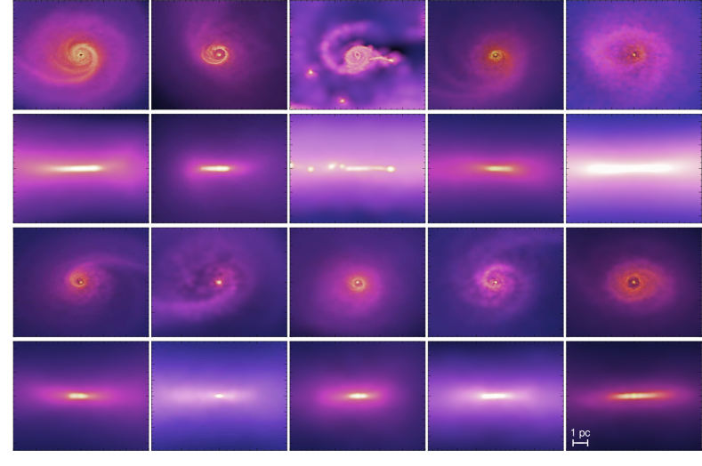
Figure 1: The face-on (x-y) and edge-on (x-z) disk structure of the nuclear disks in several representative simulations. Scale is the same in all panels (lower right). Each example is a simulation of the central $\sim 100\,$pc of galaxy nuclei with different initial large-scale galaxy properties (inflow-to-BH mass ratios, gas fractions, and treatments of stellar feedback; details in text). Intensity encodes gas surface density (increasing from $N_{H}\lesssim 10^{21}\,{\rm cm^{-2}}$ to $N_{H}\gtrsim 10^{25}\,{\rm cm^{-2}}$. Colors encode the absolute star formation rate of the gas (increasing from blue to red/yellow). The formation of a lopsided, gas-rich disk is ubiquitous. Regions where gas shocks (edges in this image) dissipate energy, leading to rapid gas inflow. Viewed edge-on, the disks are all thick, with columns $\gtrsim 10^{22}\,{\rm cm^{-2}}$ to $h/R\sim$unity.

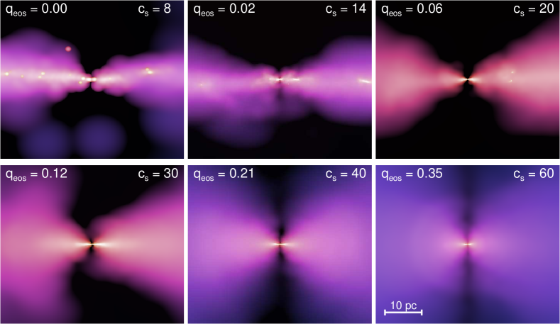
Figure 2: Edge-on gas mass distribution plotted in cylindrical coordinates $(R,\,z)$ to highlight the torus-like structure of the disk, with intensity and color as Figure 1. The simulations shown here are a survey of $q_{\rm eos}$, which determines the effective (sub-grid) pressure support of the ISM: the (mass-averaged) effective sub-grid sound speed $c_{\rm s}$ is labeled in each panel. Figure 1, for some of our survey of $q_{\rm eos}$. As expected, the systems become more puffed-up with increasing $q_{\rm eos}$ (sub-grid $c_{s}$), and for $q_{\rm eos}\gtrsim 0.4$ they are nearly spherical. But at small $q_{\rm eos}$, the scale heights do not decrease as rapidly as $\propto c_{s}$, but approach some asymptotic minimum.

Figure 1 shows some illustrative examples of the nuclear gas disks that form around the BH radius of influence in our simulations. We plot gas surface density maps, with color encoding the gas effective sound speed, from scales of $\gtrsim 10\,$kpc to $<1\,$pc. The initial large-scale simulation in this case is a fairly gas-rich major merger of two $\sim L_{\ast}$ galaxies (with initial bulges of mass $1/3$ the disk mass and BHs of mass $10^{7}\,M_{\sun}$). The zoom-in simulations were carried out just after the coalescence of the two nuclei, which is near the peak of star formation activity, but when the system is still quite gas rich.

We both show the global structure, and edge-on $(R,\,z)$ disk. The scales shown include the BH radius of influence, about $10\,$pc in these galaxies. In the face-on projection, the $m=1$ modes that form at these scales are clearly evident. They drive large torques on the gas, driving inflow into $\ll 0.1\,$pc at accretion rates as high as $10\,M_{\sun}\,{\rm yr^{-1}}$ in these simulations, sufficient to power the most luminous quasars (see Figures 5 & 13 in Hopkins & Quataert (2010a)).

Here, however, we note the broad resemblance of these nuclear disks to the canonical AGN “torus.” The disks are thick, with characteristic scale $\sim 0.1-10\,$pc, gas masses $\sim M_{\rm BH}$, and scale heights of order unity. Of course, unlike in toy models of the torus, the gas is part of a continuous distribution at all radii, and its structure is non-trivial.

4 Vertical Structure: Dependence on Stellar Feedback

4.1 Overview

The major input parameter of our models is the parameterization of the effects of stellar feedback on the ISM. This is accomplished, here, with the parameter $q_{\rm eos}$ described in § 2, that allows us to interpolate between a feedback-free ISM and one with large non-thermal internal gas velocities and pressures driven by stellar feedback.

The so-called torus is defined largely by its vertical structure, which determines the obscured fractions. To the extent that the amount of turbulent velocity and pressure support in the simulated gas is defined by a sub-resolution model, we must ask whether the vertical structure we see in our simulations is entirely a consequence of our model inputs, or whether there are robust statements and predictions we can make.

We therefore consider the vertical structure in detail, in a specific survey of $q_{\rm eos}$. This survey (Nf8h2b4q in Hopkins & Quataert 2010a) is a typical, canonical set of conditions ($3\times 10^{7}\,M_{\sun}$ BH, with disk-to-BH mass ratio of a few inside $\sim 100\,$pc initially, and initial gas fraction $\sim 50\%$, typical of the simulations in Figure 1). We re-simulate the identical cases, but with $q_{\rm eos}=0.0$, $0.018$, $0.06$, $0.10$, $0.12$, $0.15$, $0.21$, $0.25$, $0.35$, $0.60$, $1.0$. The spacing in $q_{\rm eos}$ is chosen such that the implied turbulent gas sound speeds are spaced over roughly equal logarithmic intervals from the minimum $q_{\rm eos}=0$ floor ($10\,{\rm km\,s^{-1}}$) to the maximum $q_{\rm eos}=1$ value (which is density dependent, but $\sim 100\,{\rm km\,s^{-1}}$ at range of interest).

Figure 2 shows the edge-on ($R,\,z$) gas structure, as a function of $q_{\rm eos}$. A few generic features stand out. The disks are generally thick. At the smallest radii ($\lesssim 0.1-1\,$pc), they eventually become thin, since the gravity from the BH becomes arbitrarily strong. This gives a torus-like morphology. Flares (discussed below) and lopsidedness (reflecting the lopsided disk mode on these scales) are not uncommon. As a function of $q_{\rm eos}$, we see unsurprisingly that the gas distribution becomes more smooth and vertically extended at higher $q_{\rm eos}$. For $q_{\rm eos}\gtrsim 0.4$, the system is no longer really a vertically supported disk, but spherical – however, as discussed in Hopkins & Quataert (2010a), this is likely an unrealistically large implicit feedback efficiency.

The most surprising thing about Figure 2 is how little change there is as a function of $q_{\rm eos}$. For $q_{\rm eos}\sim 0-0.35$, there is a factor of $\sim 5$ change in $c_{s}$, which leads to a naive expectation of a factor of $\sim 5-25$ change in $h/R$. We see much weaker variation. We now consider this quantitatively.

4.2 General Expectations

To inform our comparisons, consider a simple smooth, isothermal system, in which the self-gravity of the gas is negligible (i.e. the potential is dominated by the BH, stars, and/or dark matter). The equation of vertical hydrostatic equilibrium

$$\frac{\partial P}{\partial z}=c_{s}^{2}\,\frac{1}{\rho}\,\frac{\partial\rho}{\partial z}=-\frac{\partial\Phi}{\partial z}$$ (1)

then has the trivial solution

$$\rho(R,z)=\rho_{0}(R)\,\exp{\left\{c_{s}^{-2}\,[\Phi(R,0)-\Phi(R,z)]\right\}}\ .$$ (2)

For large $z/R$, this depends on the specific form of $\Phi$, and so on the details of the global mass distribution. However, if the disk is thin, i.e. most of the mass is at $z/R\ll 1$, then this has a particularly simple expression. For any background spherical mass distribution, we have $\partial\Phi/\partial z=(\partial\Phi/\partial r)\,(\partial r/\partial z)=(V_{c}^{2}/r)\,(z/r)$, where $r^{2}=R^{2}+z^{2}$ and $V_{c}^{2}=G\,M_{\rm enc}(<r)/r$. So for $z\ll R$, $\Phi(R,0)-\Phi(R,z)\approx G\,M_{\rm enc}(<R)\,R^{-2}\,z/2\approx V_{c}^{2}\,(z/R)^{2}/2$.

Together, this gives the especially simple solution for the density for a quasi-spherical potential:

$$\rho(R,z) \approx\rho_{0}(R)\,\exp{\left\{-\frac{1}{2}\,\left(\frac{z}{h_{s}}\right)^{2}\right\}}$$ (3)

$$\frac{h_{s}}{R} \equiv\frac{c_{s}}{V_{c}}=c_{s}\,\left(\frac{G\,M_{\rm enc}(<R)}{R}\right)^{-1/2}$$ (4)

Of course, the $c_{s}$ here does not need to be thermal. Non-thermal pressure sources such as turbulent motions will have the same effect. So for comparison with simulations we should take $c_{s}\rightarrow c_{z,\,\rm eff}$, where $c_{z,\,\rm eff}^{2}=c_{s}^{2}+\sigma_{z}^{2}$ includes both the thermal and/or sub-resolution effective sound speed ($c_{s}$) and resolved turbulent vertical motions ($\sigma_{z}$).

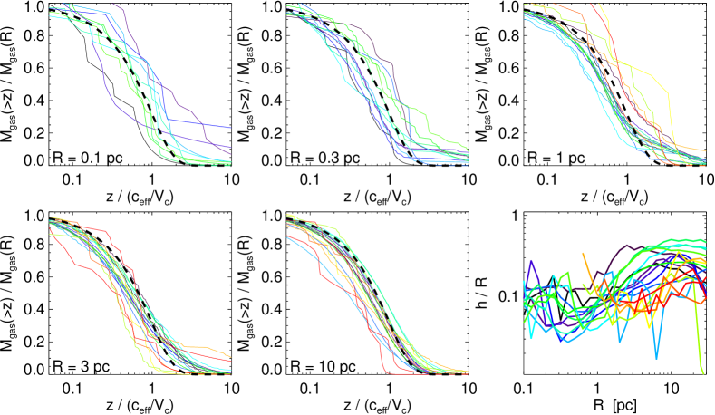
Figure 3: Vertical gas mass distribution at different radii. Panels show the integrated gas mass fraction ($M_{\rm gas}(>|z|)/M_{\rm gas}$) above a given height $|z|$, for gas in a narrow radial annulus about $R$ (each $R$ labeled). The heights are normalized to the expected scale height $z_{0}=c_{\rm eff}/V_{c}$, where $c_{\rm eff}=(c_{s}^{2}+\sigma_{z}^{2})^{1/2}$, where $c_{s}$ is the sub-grid velocity dispersion (plus thermal sound speed) and $\sigma_{z}$ is the resolved gas velocity dispersion. Each line is a different simulation (with varied initial gas fraction, disk and BH mass, sub-grid equation of state, and star formation laws); shown at a randomly-chosen time near the peak of the inflow onto the BH (but behavior is similar over the entire duration of the simulations). Thick dashed black line is the simple Gaussian expectation for an isothermal gas disk with weak self-gravity in vertical equilibrium (Equation 3). Bottom Right: The scale height $h$ (best-fit dispersion $z_{0}$, fitting the vertical gas distribution at each radius to a Gaussian), as a function of radius, for each simulation. The scale heights are significant, and the vertical behavior approximately follows the linear expectation at these radii, if the full vertical dispersions are included.

Figure 3 compares this expectation for $\rho(z)$ as a function of $c_{z,\,\rm eff}/V_{c}$ to the actual vertical mass distribution measured in narrow radial annuli from $\sim 1-10\,$pc. We use the full $c_{z,\,\rm eff}$ as defined above. The distributions are reasonably described by the above scalings, A gaussian core is typical, with a slightly broader (often more exponential) distribution at high-$z$. Remember that at sufficiently large $|z|$, the correct solution involves the full potential; if we account for this more accurately, we see similar agreement. The important point is that the gas does appear to be in vertical equilibrium.

4.3 Gravitational Support

Given the gas dispersion $c_{z,\,\rm eff}$ in the simulations, the vertical structure is what we would expect. But are these dispersions primarily sub-resolution (set by the model), thermal, or gravitational in origin?

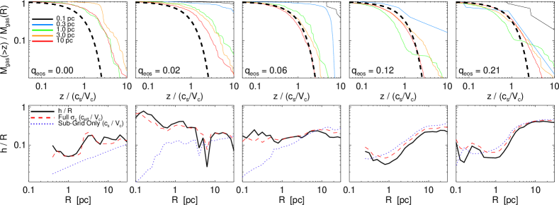
Figure 4: Top: Vertical gas distribution, in our survey of $q_{\rm eos}$. Each panel shows a different simulation in the $q_{\rm eos}$ survey. Each line shows the vertical gas distribution at a different radius (as labeled). Here, the x-axis is scaled only by $c_{s}/V_{c}$, the scale height expected if the sub-resolution (feedback-driven) velocity dispersions were dominant (as compared to $c_{\rm eff}$). Bottom: Gas scale height $h$ versus radius (solid black lines). Dotted blue lines show the expected height if just the subgrid velocities were present. Dashed red lines compare the expected height including the full resolved dispersion $c_{\rm eff}$. In large-$q_{\rm eos}$ systems, the implicit feedback dominates the vertical support. But the scale heights in low-$q_{\rm eos}$ systems are supported by large resolved turbulent vertical velocities, despite the lack of feedback. There is some non-feedback dispersion source in these systems.

Figure 4 again considers the vertical gas profile, but in our survey of different $q_{\rm eos}$. We know from Figure 3 that accounting for the full gas motion explains the observed scale heights. Therefore here we compare the expectation if the gas motions were purely thermal and/or sub-resolution – i.e. $c_{z\,\rm eff}=c_{s}$, where $c_{s}$ is the sound speed and is dominated by the sub-resolution turbulent effective $c_{s}$ (since the explicit cooling time of the gas is $\sim 10^{4}$ times shorter than its dynamical time).

In the higher-$q_{\rm eos}$ (higher effective $c_{s}$) simulations, this explains most of the pressure support, i.e. the resolved turbulent dispersion $\sigma_{z}\ll c_{s}(\rm sub-grid)$. But at low $q_{\rm eos}$, the scale heights and $c_{z,\,\rm eff}$ do not drop nearly as quickly as the sub-grid $c_{s}$ alone. There is some non-thermal, resolved gravitational process giving rise to minimum scale heights and vertical dispersions.

What, then, dominates the effective vertical “heating” in the torus region?

4.3.1 Clump-Clump Encounters

It has been proposed that two-body scattering between dense molecular clumps in the gas could maintain the observed scale heights (Krolik & Begelman, 1988; Nayakshin & King, 2007; Hobbs et al., 2010). However, we find these effects are negligible in our simulations.

Consider clumps within the plane of a disk. Scattering a clump to large $V_{z}\sim V_{c}$ requires both (a) an encounter between two clumps with relative velocity $\gtrsim V_{c}$, and (b) an encounter within an impact parameter $b$ such that $G\,M_{\rm cl}/b\,V_{c}\gtrsim V_{c}$. The mean time per clump between such encounters is just $\tau^{-1}\sim f(V_{c}/\sigma)\,n_{\rm cl}\,b^{2}\,V_{c}$, where $n_{\rm cl}$ is the volume density of clumps and $f(V_{c}/\sigma)$ is the fraction of the clumps moving on orbits with large non-circular motions ($|V-V_{c}|\gtrsim V_{c}$). If the system is sufficiently thin such that $b>h$, the disk thickness, then this becomes $\tau^{-1}\sim f(V_{c}/\sigma)\,dN_{\rm cl}/dA\,b\,h\,V_{c}$. Using $n_{\rm cl}=\bar{\rho}_{\rm gas}/M_{\rm cl}=\Sigma_{\rm gas}/h\,M_{\rm cl}$, the maximum $b$ above, and $V_{c}^{2}\sim G\,M_{\rm enc}/r$, this can be written

$$\Omega\,\tau\sim\frac{1}{f(V_{c}/\sigma)}\,\left(\frac{M_{\rm enc}}{M_{\rm gas}}\right)\,\left(1+Q\,N_{\rm cl}\right)$$ (5)

where $Q$ is the Toomre $Q\sim(h/R)\,(M_{\rm gas}/M_{\rm enc})^{-1}$ and $N_{\rm cl}$ the total number of clumps, and the expression shown interpolates between the extremely-thin and thick-disk cases. For a Maxwellian velocity distribution, $f(V_{c}/\sigma)\sim\exp{\{-(V_{c}/\sigma)^{2}/2\}}$. Since both $f(V_{c}/\sigma)$ and $M_{\rm gas}/M_{\rm enc}\sim M_{\rm gas}/M_{\rm BH}$ are small at this radius, collisions require many dynamical times. But any induced vertical heating will relax away in just a single or couple dynamical times, since the cooling time is much shorter than the dynamical time. So without continuous energy input to drive large dispersions – which is essentially the problem we wished to solve in the first place – this mechanism fails.

Moreover, if star formation occurs with some efficiency relative to the dynamical time ($\dot{\rho}_{\ast}\sim\epsilon\rho\,\sqrt{G\,\rho}$, with $\epsilon\sim 1-10\%$), then using the fact that any clump must have $\rho\gtrsim M_{\rm enc}/R^{3}$ to avoid tidal destruction, clump-clump gas heating must occur faster than the gas exhaustion timescale in a clump, requiring

$$\left(\frac{M_{\rm gas}}{M_{\rm enc}}\right)\gg\epsilon\,(1+Q\,N_{\rm cl})\,\exp{\left\{\frac{1}{2}\left(\frac{V_{c}}{\sigma}\right)^{2}\right\}}$$ (6)

Even for $\sigma\sim V_{c}$ (which begs the question) and an extremely thin disk $Q\,N_{\rm cl}\lesssim 1$, this requires $M_{\rm gas}/M_{\rm enc}\gg 0.1$, which is not satisfied at the inner radii $\lesssim 10\,$pc.

4.3.2 Twists and Misalignment

Figure 5: Contribution of disk mis-alignments and twists (as opposed to disk thickness) to obscuration. For each simulation in the sample shown in Figure 3, we calculate the (time-averaged) fraction of sightlines towards the BH which would be obscured ($N_{H}>10^{22}\,{\rm cm^{-2}}$) assuming the disk is razor-thin at every radial annulus $\Delta r$ (using the angular momentum vector of gas in $\Delta r$ to define the disk plane). If the disk plane (angular momentum direction) were constant with radius, this would be zero, but if the plane tilts as a function of radius, it can be non-zero (a $180^{\circ}$ flip at some radius, maintained for the duration of the simulation, would give an obscured fraction of unity). Although there are significant mis-alignments (see Hopkins et al., 2011d), and in a few systems they can account for obscured fractions $\gtrsim 50\%$, they would only give an integrated obscured fraction of $\sim 25\%$ if the disk were thin at all radii. And even simulated cases with no “twists” still have large obscured fractions and $h/R$ in Figure 3. The torus must actually be thick to match observations – so some process must explain large scale-heights in the gas.

Another possibility is that large covering factors are maintained by virtue of the fact that the nuclear disk is mis-aligned with the larger-scale inflow/bar/disk. This is particularly interesting because observations find relatively little correlation between the axes of AGN (traced by jets or the torus) and the inclination of the host galaxy (e.g. Keel 1980; Lawrence & Elvis 1982; Schmitt et al. 1997; Simcoe et al. 1997; Kinney et al. 2000; Gallimore et al. 2006; Zhang et al. 2009; but see also Maiolino & Rieke 1995; Shen et al. 2010 and references therein). In a companion paper, Hopkins et al. (2011d), we show that this lack of alignment is reproduced in our simulations owing to two processes. First, occasionally the central gas supply is strongly influenced by a single or couple large clumps that form at large radii, fragment and sink, realigning the central angular momentum vector (see e.g. Nayakshin & King, 2007). Examples of this have also been seen in cosmological zoom-in simulations (Levine et al., 2010). Second, even in smooth flows, the secondary and tertiary gravitational instabilities will tend to de-couple their angular momentum from the primary (external) bar/spiral structure, and semi-chaotically precess or tumble in three dimensions (see Heller et al., 2001; Shlosman & Heller, 2002; El-Zant & Shlosman, 2003; Maciejewski & Athanassoula, 2008; Englmaier & Shlosman, 2004).

In Figure 5 we show how this can contribute to obscuration. It is straightforward to measure the axis of angular momentum of the disk in a radial annulus, and define the corresponding inclination $\Theta(r)$ (relative to the initial, uniform angular momentum axis of the entire initial disk). We also know the mass $\Delta M_{\rm gas}(r)$ enclosed in each annulus; we can simply integrate along all sightlines towards the BH, assuming the mass is in an axisymmetric razor-thin disk with inclination $\Theta(r)$, to obtain the column density $\Sigma_{\rm gas}$ along each sightline. If a sightline is covered by the disk at some radius, it is “obscured.”

We consider these assumptions because they effectively define a minimum obscured fraction stemming purely from twists and misalignments. This fraction can be considerable, but there is a broad range in different simulations – many systems have only $<20\%$ covering fractions, but there is a long tail towards near full covering (anti-alignment of the central and outer disks). Integrated over all simulations and snapshots, the average covering fraction is $\approx 25\%$. A warped or twisted disk can therefore yield large covering angles towards the BH even when the disk itself is thin.

However, this is not the full story. First of all, the covering fractions of $\approx 25\%$ are still significantly lower than the total covering fraction of obscuration in the simulations, by a factor of at least $\sim 2$. Moreover the cases with weak twists ($\ll 20\%$ covering in Figure 5) still exhibit large obscured fractions and thick disks. The key point is that the vertical density distribution in Figures 3-4 shows that we must explain the actual thickness, not just the orientation of the disks. This is true for observations as well – empirical modeling of the hot dust continua indicates that the obscuring region must be geometrically thick, not just a misaligned larger-scale thin disk (e.g. Deo et al., 2009, and references therein). A time-dependent twist can, in principle, “pump up” vertical motions, but fast cooling times make it difficult to sustain a large scale height anywhere except close to the location of the twist (where the pumping occurs). Some mechanism that pumps vertical motion throughout the disk, on a timescale comparable to the local dynamical time, is required.

4.3.3 Bending Modes

Bending modes can provide an efficient channel for “heating” the torus. Their behavior is particularly interesting in response to “slow modes” in a quasi-Keplerian potential. Consider a general bending mode

$$h(R,\phi,t) =H(R)\,\exp{\left\{i\,\left(\omega_{b}\,t-m_{b}\,\phi\right)\right\}}$$ (7)

$$H(r) =h_{0}(R)\,\exp{\left\{i\,\int^{R}k_{b}(R^{\prime}){\rm d}R^{\prime}\right\}}$$ (8)

in a system that includes some quasi-spherical component (BH+bulge+halo) and a thin disk with surface density $\Sigma_{d}$, angular (vertical) frequency $\Omega$ ($\nu$), and velocity dispersions in the radial, azimuthal, and vertical directions $\sigma_{r}$, $\sigma_{\phi}$, $\sigma_{z}$. The value $k_{b}$ is the radial wavenumber of the bending mode, and $m_{b}$ is its azimuthal wavenumber. In the WKB regime, if $\sigma_{r}^{2}\gtrsim\sigma_{\phi}^{2}$, the dispersion relation can be written

$$(\omega_{b}-m_{b}\,\Omega)^{2}=\nu^{2}+2\pi\,G\,\Sigma_{d}\,|k_{b}|+(\sigma_{z}^{2}-\sigma_{r}^{2})\,k_{b}^{2}$$ (9)

(Kulsrud & Mark, 1970; Kulsrud et al., 1971; Mark, 1971; Poliachenko, 1977).

If $\sigma_{r}$ is sufficiently large, the system is vulnerable to the so-called “firehose” instability and bending modes will be self-excited. However, it is unusual to see such large $\sigma_{r}$ (and $\sigma_{r}^{2}>\sigma_{\phi}^{2}$) in disks. Even with large $\sigma_{r}$, the fact that $\sigma_{r}<V_{c}(r)$ for any meaningful “disk” means that usually, when the self-gravity of the disk is small compared to the background potential, the system is stable. And in even in self-gravitating disks with large $\sigma_{r}$, it typically takes only a small $v_{z}$ to stabilize them, so the induced $h/R$ is not large.

However, consider the special case of interest here, where the disk is quasi-Keplerian and has a large lopsided mode driving accretion. The system is (initially) a thin disk in the quasi-Keplerian potential of a BH – i.e. to lowest order, the parameters are those of a pure Keplerian potential, with some correction terms that scale with $M_{d}/M_{\rm BH}$ of $\mathcal{O}(\epsilon)\ll 1$. As discussed above, and in previous works, the disk develops a gravitational instability in the disk plane (the standard density waves of spiral/bar/etc. modes), which we can describe by e.g. the perturbed density field $\Sigma_{1}(R,t)=|a|\,\Sigma_{0}(R)\,\exp{\{i\,(\int^{R}k_{p}(R^{\prime}){\rm d}R^{\prime}+\omega_{p}\,t-m_{p}\,\phi)\}}$. Here $|a|$ is the effective mode amplitude in the density field at $R$, and the properties $\omega_{p}$, $m_{p}$, and $k_{p}$ refer to the frequencies and wavenumbers of this, in-plane mode (independent from the $\omega_{b}$, $m_{b}$, and $k_{b}$ of the bending mode). The fact that the potential is quasi-Keplerian, i.e. has $\Omega\approx\kappa$, favors (and supports for long periods of time) global, “slow” $m=1$ modes – modes with $m_{p}=1$, $\omega_{p}\sim\epsilon\,\Omega\ll\Omega$, and $|k_{p}\,R|\sim 1$. These are the lopsided/eccentric modes that we see above. The potential of the BH+disk system is

$$\Phi(r)=-\frac{G\,M_{\rm BH}}{r}+\Phi_{d}(r)$$ (10)

and it is useful to define the parameter

$$\varomega \equiv\frac{\Omega^{2}-\kappa^{2}}{2\,\Omega}=-\frac{1}{2\,\Omega}\,\left(\frac{2}{r}\,\frac{d}{dr}+\frac{d^{2}}{dr^{2}}\right)\Phi_{d}\ .$$ (11)

To first order in $\epsilon$, then, the WKB dispersion relation of such modes in a cold ($c_{s}\ll V_{c}$) disk is

$$\omega_{p}=\varomega+\pi\,G\,\Sigma_{d}\,|k_{p}|\,\Omega^{-1}$$ (12)

(Tremaine, 2001). The equations of motion for the perturbed velocity ${\bf v}=R\,\Omega\,\hat{\phi}+v_{r}\,\hat{R}+v_{\phi}\,\hat{\phi}$ become, at this order,

$$v_{r} =-\frac{i}{2\,(\omega_{p}-\varomega)}\,\left(\frac{{d}\Phi_{1}}{{d}r}+\frac{2\,\Phi_{1}}{r}\right)=-\frac{\Sigma_{1}}{\Sigma_{d}}\,\Omega\,|k_{p}|^{-1}$$ (13)

$$v_{\phi} =\frac{i}{2}\,v_{r}$$ (14)

where we have used the WKB relation $\Phi_{1}\approx-2\pi\,G\,|k_{p}|^{-1}\,\Sigma_{1}$. Since $\sigma_{r}^{2}=\langle|v_{r}|^{2}\rangle$ and $V_{c}=\Omega\,R$, this becomes just

$$\sigma_{r}=|a|\,|k_{p}\,R|^{-1}\,V_{c}$$ (15)

with $\sigma_{r}^{2}=4\,\sigma_{\phi}^{2}$. And recall for our simulations, the magnitude $|a|$ in the disk is order unity during the active phases of BH growth (Hopkins & Quataert, 2010a).

This is the important point – because of cancellations that occur (essentially the entire system is near-resonance), the radial induced velocities from the $m=1$ mode are quite large, $\sim V_{c}$, independent of how small the ratio $M_{d}/M_{\rm BH}$ may be.

Now return to the dispersion relation for bending modes. For the non-disk (Keplerian) part of the potential, $\nu^{2}=\Omega^{2}$. To leading (zeroth) order in $\epsilon\sim M_{d}/M_{\rm BH}$, then, the dispersion relation becomes

$$\left(\frac{\omega_{b}}{\Omega}-m_{b}\right)^{2}=1+\left[\left(\frac{h}{R}\right)^{2}-|a|^{2}\,|k_{p}\,R|^{-2}\right]\,|k_{b}\,R|^{2}$$ (16)

where we have defined $h/R=\sigma_{z}/V_{c}$.

Recall, $|a|\,|k_{p}\,R|^{-1}\sim 1$ for the lopsided disk mode, and $|k_{b}\,R|\gg 1$ in the WKB limit – thus, whenever the disk is thin, the radial motions induced by the $m_{p}=1$ eccentric disk excite bending modes. These bending modes will grow on the local dynamical timescale, since $\omega_{b}\sim\Omega$. Compare the slow modes in the plane, which have $\omega_{p}\sim\epsilon\,\Omega$ and can be long-lived.

The bending mode, of course, creates some non-trivial vertical motion. The growth of the mode will saturate when it drives a $\sigma_{z}$ sufficiently large so as to reach the marginal stability condition of Equation 16 (Im$(\omega_{b})=0$), which we can write as

$$\left(\frac{h}{R}\right) \rightarrow|k_{b}\,R|^{-1}\,\left(|a|^{2}\,|k_{p}\,R|^{-2}\,|k_{b}\,R|^{2}-1\right)^{1/2}$$ (17)

$$\approx\frac{|a|}{|k_{p}\,R|}\sim|a|$$ (18)

where the second equality uses $|k_{b}\,R|\gtrsim 1$. In short, tightly-wound bending modes arise, and saturate $v_{z}$ at a large fraction of $V_{c}$, such that $h/R$ is driven to order unity wherever the eccentric mode persists, independent of the degree of self-gravity of the disk!

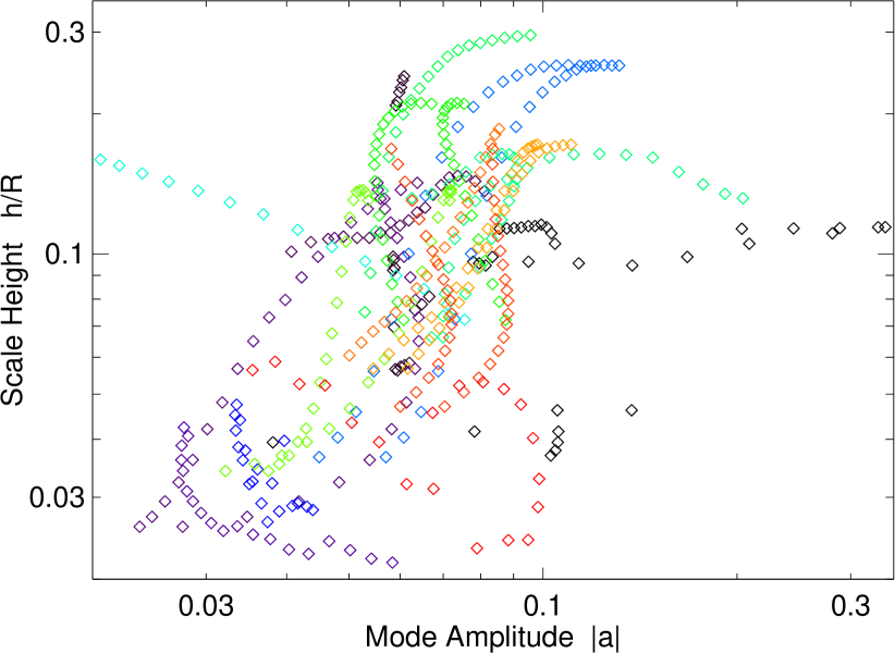
Figure 6: Comparison of the scale-height $h$ (as in Figure 3) to the $m=1$ eccentric disk mode amplitude $|a|\equiv|\Sigma_{1}/\Sigma$, at different radii (each point samples radii evenly in $\log{R}$ from $R=1-10\,$pc), for different simulations (each color denotes a different simulation, near its peak activity). All simulations shown are “cold” (i.e. have weak stellar feedback assumed in their sub-resolution prescription, specifically $q_{\rm eos}<0.1$), so that the scale height is dominated by resolved turbulent vertical motions, not the feedback model input. In these cases, there is a correlation of the form $h/R\sim|a|$, corresponding to the prediction from an $h/R$ pumped-up by bending modes, themselves excited by radial motions from the in-plane eccentric mode. The torus height can be continuously sustained by exchange of energy from the eccentric/lopsided disk mode that powers the accretion onto the BH.

In Figure 6, we check whether this prediction at all describes our simulations. We compare the scale height $h/R$ to the measured mode amplitude $|a|$ of the in-plane $m=1$ mode, at a random time during the active phase, for each of a subset of our simulations. We chose only the simulations for which $q_{\rm eos}\leq 0.1$, where we can confirm that the sub-grid assumed $c_{s}$ does not dominate $c_{\rm eff}$ or the vertical scale height on the scales we measure (see Figure 4). We sample both quantities at even intervals in $\log{R}$ from $R=0.3-10\,$pc. There is, unsurprisingly, large scatter, but a correlation is significant at $>3\,\sigma$ and consistent with $h/R\sim|a|$ over most of the simulated range. That the relation is not exactly linear at the high-$h/R$ end and shows considerable scatter is expected, both because of contributions from $k_{b}$ and $k_{\rho}$ in the derivations above, non-linear effects (especially at $h/R$ and/or $|a|$ $\gtrsim 0.1$), and some non-zero support from $c_{s}$. But it is quite unlikely that this relation would arise accidentally – after all, for otherwise equal properties, a lower-$h/R$ disk is actually more gravitationally unstable, so if anything we would naively expect the inverse of the observed correlation.

5 Basic Dynamical Properties of the “Torus”

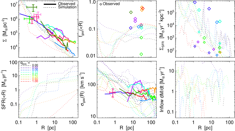
Figure 7: Azimuthally-averaged nuclear disk properties versus radius. Each dotted line is a simulation with different galaxy and inflow properties, but one where some nuclear inflow is excited. We chose a random time near the peak of activity for each simulation to show here, but the results are similar over the entire active phase of each. Here for a set of simulations with identical initial conditions but varied $q_{\rm eos}$, the parameter describing our effective equation of state and stellar feedback model. Lines range from black ($q_{\rm eos}=0$; effective $c_{s}=10\,{\rm km\,s^{-1}}$) to red ($q_{\rm eos}=1$; effective $c_{s}=100\,{\rm km\,s^{-1}}$), evenly spaced in $\log{c_{s}}$. Top Left: Surface mass density profiles. Points with error bars show constraints from AGN maser disks (NGC 3079; Kondratko et al., 2005, magenta), (NGC 3393; Kondratko et al., 2008, dark green), (NGC 1068; Lodato & Bertin, 2003, pink), (Circinus; Greenhill et al., 2003, light green). Solid lines show constraints from adaptive-optics (AO) measurements of AGN (NGC 1068, 1097, 3227, 3783, 4051, 4151, 6814, 7469, Circinus; in violet, green, cyan, blue, dark green, magenta, red, orange, dark blue, respectively) (Davies et al., 2007) and Hicks et al. (2009). Top Center: Gas fraction ($M_{\rm gas}(<R)/(M_{\ast}(<R)+M_{\rm gas}(<R))$). Diamonds are the AO systems (same color styles), at the resolution limits for complementary constraints used to derive $f_{\rm gas}$. Top Right: SFR surface density. For each AO system where a measurement is available, two points are shown. The first is the current SFR (small points), second is the peak SFR (larger points), both estimated from the fits to the SFR history inside the minimum and maximum observed radii in Davies et al. (2007). Bottom Left: Integrated SFR$(<R)$. Bottom Center: Vertical velocity dispersion of the gas. Dotted lines show both the resolved and sub-grid assumed dispersions (added in quadrature). Bottom Right: Instantaneous inflow rate through $R$, generated by gravitational torques from the eccentric disk structure.

Thus far, we’ve focused on the origin of torus structural properties in simulations. We now examine these properties in more detail and compare to observations. Figure 7 shows a number of (azimuthally averaged) properties of the nuclear gas, as a function of radius. We plot the gas surface mass density, gas fraction, SFR, vertical gas velocity dispersion, and gas inflow rate $\dot{M}$ (here defined so positive is inflow). The velocity dispersion includes both resolved and sub-resolution components, i.e. $c_{\rm eff}^{2}\equiv c_{s}^{2}+\sigma_{z}^{2}$, where $c_{s}$ is the sub-grid implied sound speed (plus any thermal components) and $\sigma_{z}$ is resolved vertical dispersion.

We show this for our suite of simulations from Figure 4 in which we systematically vary the sub-grid equation of state (via the parameter $q_{\rm eos}$). For each, we select a random snapshot near the peak of inflow activity. Because the global properties – gas density profiles, inflow rates, circular velocities, etc – are primarily set by global gravitational torques (see Hopkins & Quataert, 2011a), the parameter $q_{\rm eos}$ does not appear have a dramatic qualitative effect on these properties. The primary effect is to determine the efficiency of fragmentation, which in turn changes the variability and global efficiency of star formation and gas exhaustion. If we consider the wider range of simulations shown in Figure 3, which vary the initial gas fractions, bulge-to-disk, and BH-to-disk mass ratios, we find a similar range in the predicted properties.

In more detail, Hopkins & Quataert (2011b) show that the surface density profiles that arise are a natural consequence of the dynamics of tidal torques from the $m=1$ lopsided disk instabilities. Specifically, the perturbation dynamics set a robust range of “quasi-equilibrium” profiles in which the gas mass density remains quasi-steady state over the active phase so long as there is sufficient initial inflow to trigger the process. If the profile is a power law $\Sigma\propto R^{-\eta}$, then this range is $1/2\lesssim\eta\lesssim 1$, similar to that seen in “cuspy” ellipticals.

The SFR surface density follows simply from the assumed local relation between star formation efficiency and dynamical time: in the simulations, $\dot{\rho}_{\ast}\propto\rho^{3/2}$. Competition between gas inflows and SF sets the gas fractions, although these evolve significantly via depletion.

There are some observations to which we can compare. Water masers have been observed and used to map the inner disk structure around AGN in a few nearby galaxies (Greenhill et al., 1997, 2003; Braatz et al., 2004; Henkel et al., 2005; Kondratko et al., 2006b, a, 2008). These are sensitive to densities $\sim 10^{8}-10^{9.5}\,{\rm cm^{-3}}$ (typically $\sim 0.1-1\,$pc). At larger radii, interferometry has also been used to image the molecular and HI gas in the nuclei of some nearby systems (Lonsdale et al., 2003; Schinnerer et al., 2000; Combes et al., 2004; García-Burillo et al., 2005; Schinnerer et al., 2008). Complemented with adaptive-optics imaging of nearby nuclei, this gives constraints on the gas+stellar dynamics, and information on the star formation history (Kuntschner et al., 2001; Davies et al., 2006; Sánchez et al., 2006; Davies et al., 2007; Hicks et al., 2009).

We compile these observations and compare to our simulations in Figure 7. Most of the observed systems have BHs with broadly similar masses to our $\sim 3\times 10^{7}\,M_{\sun}$. We plot the observations at all radii available. The maser observations are shown as points with error bars for resolved properties of disks outside the minimum radius enclosing the BH. The larger-scale surface densities mapped from the gas velocity fields with VLBI are shown as solid lines. For constraints involving stars (gas fractions, SFR), the VLBI+AO constraints are shown as diamonds, at the minimum resolved radii of the AO observations. The nuclear SF history is modeled for several cases in Davies et al. (2007); we show their estimated current SFR both at the innermost radii where stellar light is measured and at the outer radii where the integrated light is used to determine the SFH. We also show their estimated maximum SFR of each observed burst from the fitted SFH within the observed radius. In all cases the observations broadly bracket the simulations, albeit with larger uncertainties in $f_{\rm gas}$ and the SFH.

Of course, since these properties all scale with the dynamical properties of the system, they are all mutually correlated. A Kennicutt-Schmidt type law similar to that observed ($\Sigma_{\rm SF}\propto\Sigma_{\rm gas}^{\eta}$; for the nuclear-scale observations see Hicks et al., 2009) is effectively built into our simulations by sub-grid assumption. We have discussed extensively the gravitational origin of the dispersion ($\sigma$). But both $\sigma$ and $\Sigma$ are related to $V_{c}$, for obvious dynamical reasons, and increase at smaller radii and/or in more massive/dense systems. And $\Sigma$ is tied to $\Sigma_{\rm SF}$ via the Kennicutt relation. We therefore predict a relation between $\Sigma_{\rm SF}$ and $\sigma$ for purely gravitational dynamic reasons. In the past, such a correlation has been interpreted as evidence of stellar feedback driving the observed dispersions – we find this may not be necessary.

6 The Column Density Distribution: To Clump or Not to Clump?

Thus far, all of our analysis has concerned global properties of the simulated torii, which we have reason to believe should be robust to the exact micro-structure of gas on unresolved scales. However, sub-resolution structure can be important in calculating the column densities observed towards the BH. We therefore consider this now with two simple sub-resolution models.

6.1 The No-Substructure Case: Smooth Torii

One extreme is trivial: we simply take the gas distribution exactly as-is from the simulations, without any assumed sub-grid substructure. The column density along a given line-of-sight at each time can then be simply determined (following Hopkins et al., 2005c). We generate $\sim 1000$ radial lines-of-sight (rays) uniformly spaced in solid angle and with its origin at the BH, and integrate the line-of-sight density until outside the galaxy.

This assumption maximizes obscuration, since locking mass up in sub-resolution clumps would confine mass to smaller covering fractions (see the discussion from simulations in Hopkins et al., 2005a).

6.2 The Clumpy Torus

In fact, we know that there must be sub-structure in the gas, because cooling and star formation occur. Most of the mass in the ISM is probably locked into dense cold clumps. Unfortunately our simulation, limited by the physics included, does not predict the clump properties but only indirectly assumes an effective ISM state. However, with some simple assumptions, we can construct a sub-resolution estimate of all the relevant clump properties, without the introduction of any tunable parameters.

Assume temporarily that most of the mass in the ISM is locked into $N_{\rm cl}$ dense clumps, with median mass $M_{\rm cl}$, size $R_{\rm cl}$, and mean density $\rho_{\rm cl}=M_{\rm cl}/(4\pi/3)\,R_{\rm cl}^{3}$. Define the density contrast $\rho_{\rm cl}=x\,\bar{\rho}$, with respect to the volume-average background density $\bar{\rho}$. We make two assumptions, both just at the order-of-magnitude level: that the clumps are quasi-virial, and that they are in pressure equilibrium with the external medium. The first implies that whatever supports the clump generates an effective pressure $P_{\rm cl}\sim\rho_{\rm cl}V_{\rm cl}^{2}$ where $V_{\rm cl}^{2}\sim G\,M_{\rm cl}/R_{\rm cl}$. But this is just $P_{\rm cl}=G\,\Sigma_{\rm cl}^{2}$, where $\Sigma_{\rm cl}$ is the column density through the clump $\sim\rho_{\rm cl}\,R_{\rm cl}$. To within a factor of two or so, this is even true for clumps in free-fall collapse, so is likely to be robust. We know the external effective (volume-average) pressure of the medium, $P_{\rm eff}$ – this is just the volume-average pressure used for all SPH calculations. It is straightforward to then set $P_{\rm cl}\sim P_{\rm eff}$, and obtain

$$\Sigma_{\rm cl}=\sqrt{P_{\rm eff}/G}\ .$$ (19)

Pressure equilibrium is a less certain assumption, but if we were to force a mass-radius or linewidth-radius relation similar to the observed Larson’s laws in GMCs ($\sigma\propto R^{1/2}$), we would obtain the same dimensional scalings. Assuming that clumps follow the Jeans mass and radius in a self-regulating $Q=1$ disk actually also results in the same dimensional scalings, so it may be robust in a variety of regimes.

The probability of a path length $\Delta r$ intersecting a cloud is given by $p=(N_{\rm cl}/V_{\rm tot})\,\sigma_{\rm cl}\,\Delta r$, where $V_{\rm tot}$ is the total volume, and $\sigma_{\rm cl}\sim\pi\,R_{\rm cl}^{2}$ the clump cross section. But since $N_{\rm cl}\sim M_{\rm tot}/M_{\rm cl}$, this simply reduces to

$$p_{\rm cl}\sim\bar{\rho}\,\Sigma_{\rm cl}^{-1}\,\Delta r=\bar{\rho}\,(P_{\rm eff}/G)^{-1/2}\,\Delta r\ .$$ (20)

The only two quantities we ultimately care about, the probability of intersecting a clump, and the clump column, have the useful feature that the clump density contrast and number of clumps completely cancel out. Thus, for any system where the mass is concentrated in quasi-virial, pressure-equilibrium clumps, we can determine the column density distribution and probability of sightlines seeing clumps based only on reference to well-determined volume-average gas properties in the simulations ($\bar{\rho}$ and $P_{\rm eff}$). Of course, the external pressure is set in part by our adjustable $q_{\rm eos}$, so it is important to examine the consequences of that choice. Higher-order detailed radiative transfer effects will depend on the specific clump sizes and other internal properties, but these are not our focus here. Because of the cancellation of the exact size and density contrast (and correspondingly clump mass), the above relations hold for an arbitrary spectrum of clump masses, sizes, and/or densities.

The column density along a given line-of-sight can then be integrated outward from the BH. For each integration step $\Delta r$ along the ray (taken to be increments of $\epsilon\,h_{\rm sml}$, where $\epsilon\sim 0.01\ll 1$ and $h_{\rm sml}$ is the local smoothing length at each point), we determine the probability $p_{\rm cl}$ of intersecting a clump, and probabilistically assign the ray a collision or not. If there is a collision, the integrated column is increased by $\Sigma_{\rm cl}$. If not, the column is integrated through the “diffuse” (non-clump) phase of the ISM. The mass fraction in this phase (i.e. mass fraction not in star-forming clumps) is determined implicitly in the GADGET code (see Springel & Hernquist, 2003), but is always small and should have near-unity volume filling factor.

Whether or not these assumptions are justified in detail, this provides a useful toy model, and we show that it can account for a number of observations. Moreover, on galactic scales, the assumptions above have been borne out by a large number of independent observations (Larson, 1981; Ward-Thompson et al., 1994; Scoville et al., 1987; Solomon et al., 1987; Rosolowsky, 2007; Fuller & Myers, 1992; Andre et al., 1996; Blitz & Rosolowsky, 2006). Of course, such clumps as observed locally could not survive the tidal forces near a supermassive BH. But even on nuclear starburst scales, it appears that the star formation efficiency per clump dynamical time is low, implying they must be quasi-virial and not wildly out of pressure equilibrium (Tan et al., 2006; Krumholz & Tan, 2007). Similar constraints come from clump structure in the narrow-line region (e.g. Crenshaw et al., 2000; Rice et al., 2006). And the fact that similar dimensional scalings arise from Jeans considerations implies they are likely to be generic to within factors of a few. Finally, we note that the dynamic range in column density is so large that violations of the above assumptions would have to be more than order-of-magnitude in order to qualitatively affect our conclusions.

6.3 Column Densities: Model and Observations

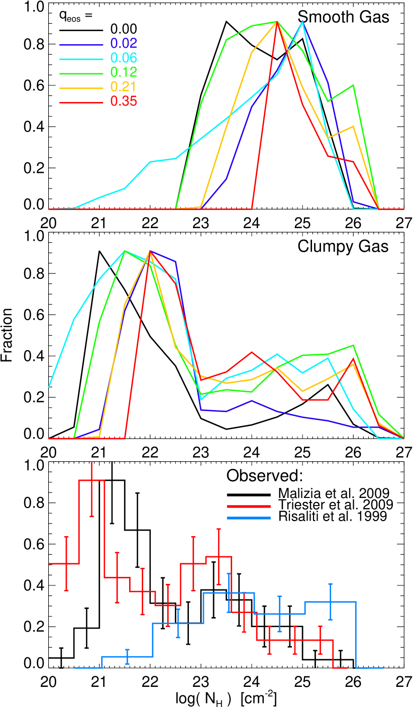
Figure 8: Top: Column density distribution predicted by our simulations. Each line is a simulation with different sub-grid equation of state (i.e. feedback/pressure support in the gas), as in Figure 7. Here, we assume there is no sub-structure in the gas (i.e. gas is perfectly smooth below our resolution limits). The obscuration is clearly over-predicted. Middle: The same, but assuming the gas is clumpy. The clumps are assumed to be quasi-virial and in pressure equilibrium with the outside medium – this completely determines the predicted $N_{\rm H}$ distribution with no free parameters. Bottom: Observational estimates of the column density distribution, from Malizia et al. (2009, black), Treister et al. (2009, red), and Risaliti et al. (1999, blue). The cutoff in these samples at $N_{\rm H}\gtrsim 10^{26}\,{\rm cm^{-2}}$ is a selection effect. Allowing for a simple clumpy gas model, without any tunable parameters, provides a good match to observed $N_{\rm H}$ distributions. Because of the effects of gravitational maintenance of $h/R$, and the global similarity of mass distributions shown in Figure 7, there is relatively little dependence of the column density distribution of $q_{\rm eos}$.

Figure 8 compares the resulting column density distribution, for simulations with varied $q_{\rm eos}$ (each sampled at a random time near their peak of accretion). We compare the distribution from the “smooth” and “clumpy” torus models above, and that observed. Because of the dynamic range in $N_{\rm H}$ predicted, we are specifically interested in comparison with samples sensitive to Compton-thick populations. We compile the (estimated intrinsic) distribution of column densities determined from the INTEGRAL/IBIS AGN sample of Malizia et al. (2009, $20-40$ keV), the predominantly SWIFT/BAT sample of Treister et al. (2009, $\sim 100\,$keV), and the nearby OIII sample in Risaliti et al. (1999) (this is a Type 2-only sample, so we normalize to their estimated total fraction of Type 2 AGN). The latter sample is most complete at the highest columns $>10^{25}\,{\rm cm^{-2}}$; none are sensitive to AGN with $N_{\rm H}>10^{26}\,{\rm cm^{-2}}$. At lower column densities, these are consistent with a wide variety of hard X-ray observations from e.g. Chandra and XMM (Ueda et al., 2003; La Franca et al., 2005; Silverman et al., 2005; Hasinger, 2008). And more recent, independent analysis of larger SWIFT/BAT samples also agrees well (Burlon et al., 2011).

Unsurprisingly, the predicted columns in the smooth torus model are uniformly large, in conflict with the observations. This is not a problem of there being “too much” gas – recall that the actual total gas masses and gas densities predicted at these scales agreed well with those in observed AGN (Figure 7). What this shows is that it is not possible to reconcile the observed central masses, gas densities, and/or SFRs of AGN with their obscured fractions, without invoking some small-scale gas clumping. The problem cannot simply be that systems are observed at different states either – as pointed out in Hicks et al. (2009), several observed optically un-obscured AGN have instantaneous near line-of-sight volume-averaged gas densities in $<1-10\,$pc that should naively imply columns of $N_{\rm H}\sim 10^{25-26}\,{\rm cm^{-2}}$, similar to our predictions here without sub-resolution clumping. And indeed direct observations on this scale have argued for such clumping (Risaliti et al., 2002; Mason et al., 2006; Sánchez et al., 2006; Nenkova et al., 2008b; Ramos Almeida et al., 2009; Hoenig & Kishimoto, 2009; Deo et al., 2011).

The column density distribution predicted by the clumpy torus model, on the other hand, agrees well with that observed. The basic features are easily understood: the small mass fraction in the diffuse ISM phase shifts the main peak in the $N_{H}$ distribution to lower values. The tail towards larger $N_{H}$ is caused by obscuration by clumps. The relative “flatness” of the tail is broadly expected for vertical profiles similar to those in Figure 3.

Although the systems plotted differ in some subtle details, there is little dependence on the parameterization of stellar feedback (our $q_{\rm eos}$ parameter). Why should the column density distribution be so insensitive to stellar feedback? Most important are the factors discussed in § 4.3, i.e. the contribution of gravitational heating which keeps the disks somewhat puffed up, and means that the gaseous scale height does not scale as strongly with $q_{\rm eos}$ as might otherwise be expected.

There are also two handy ‘conspiracies,’ in the clumpy torus scenario, which make the predicted column density distribution primarily a function of global, rather than local parameters. In the (near-polar) regime where $p_{\rm cl}\ll 1$, it is quite difficult in any model to obtain a column density radically different from those shown. This is because, even if all the mass is locked in cold clumps, a column of at least $\sim 10^{21-22}\,{\rm cm^{-2}}$ will arise just from diffuse, non star-forming galactic gas on much larger scales (see Hopkins et al., 2005b, 2006a). We do see some systematic difference in the lowest columns seen, because the exact mass in the “diffuse phase” depends on the sub-grid model – but for almost any reasonable model this mass is small, so these differences are all in the un-obscured range (and therefore dominated by or comparable to galaxy-scale effects). In the opposite (near-disk plane) regime, where $p_{\rm cl}>1$, the total column encountered is $\sim\Sigma_{\rm cl}\,p_{\rm cl}\sim\bar{\rho}\,\Delta{r}$ – i.e. in the optically thick regime the column density is simply the same as that of the “average medium,” independent of the gas properties or phase structure so long as the global dynamical properties predicted are similar (physically, this simply represents where clouds will begin to overlap, thus making a more uniform molecular medium). This is true even if we discard our assumptions of virial and/or pressure equilibrium. It is only in the intermediate column regime (which interpolates broadly between the two, so we do not expect any features or particular sensitivity to appear) where the detailed assumed model of clump properties makes some difference.

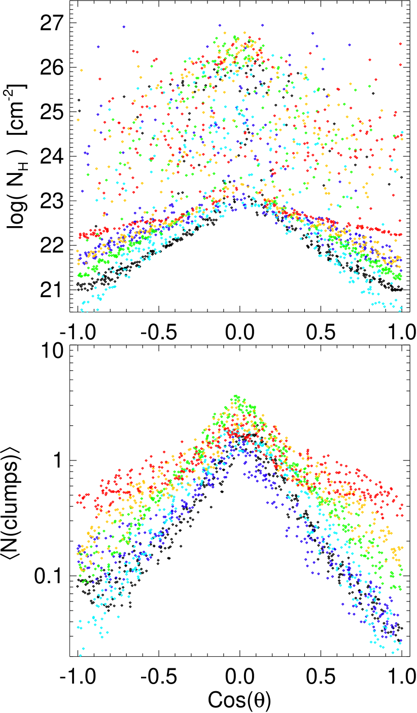
Figure 9: Obscuration properties from the clumpy-torus model in Figure 8, versus viewing angle ($\cos{\theta}=0$ is edge-on; $\cos{\theta}=\pm 1$ is polar). For $q_{\rm eos}$ survey. Top: Integrated column. Dense clusters of points at lower $N_{\rm H}$ pass through the diffuse ISM only, points scattered to higher $N_{\rm H}$ encounter clumps along the line-of-sight. The appearance of bimodality is somewhat artificial (see Figure 8; for most simulations, there are not actually two peaks). Each point is a sightline to the BH in a given simulation. Bottom: Expectation value for the number of clumps encountered along a given sightline. The clump number density is always Poisson, with $\sim$a few clumps along the typical edge-on line of sight, and rapidly declines above a scale-height of $h/R\sim 1/2$.

Figure 9 illustrates how the column density varies with inclination angle, $\theta$ (for the “clumpy” scenario). Qualitatively, the behavior is expected: columns increase towards the disk plane. There is, however, significant scatter in the column density at a given $\theta$, even within a given simulation at a given time. Strikingly similar results are seen in simulations by Wada et al. (2009), despite including a very different model for stellar feedback, and ignoring the role of self-gravity. We also show the expectation value of the number of clumps encountered along each sightline. As expected, this increases along the disk plane. Pole-on, it is $\sim 0.1\ll 1$ in almost all cases. Edge-on, it typically reaches $\sim$ a few.

These values are consistent with various indirect constraints from attempts to model AGN SEDs (Mason et al., 2006; Shi et al., 2006; Thompson et al., 2009; Ramos Almeida et al., 2009; Mor et al., 2009; Hoenig & Kishimoto, 2009; Nenkova et al., 2008a, b). Almost universally, these studies have found that a similar clumpy torus is required, with a number of clumps of order several along the edge-on lines of sight, characteristic locations/outer radii of most of the clumps from $\sim 1-100$ pc from the BH, and (where constrained) radial clump distributions with roughly power-law scaling $dp/dr\sim r^{-1}$. We find, for our typical gas surface density profiles $\Sigma_{\rm gas}\propto r^{-(0.5-1)}$, a $dp/dr\sim r^{-(0.7-1.2)}$ over the dynamic range of interest here.

The number of clumps can be crudely estimated from Eqn. 20. It is straightforward to show that this equation reduces to $\langle N_{\rm clumps}\rangle=\int p_{\rm cl}\,dr\sim(R/h)\,Q^{-1/2}$ where $h\approx c_{s}/\Omega$ is the scale height of the torus and $Q$ is the usual Toomre $Q$. For a self-regulating disk, therefore, with $Q\sim 1$, we naturally expect $\langle N_{\rm clumps}\rangle\sim(h/R)^{-1}\sim$ a few. The same scaling pertains if we discard pressure equilibrium and instead assume clumps are characteristically Jeans-scale in a $Q\sim 1$ disk (since then the scale of clumps within $R$ is $\sim h$).

The characteristic value of a few clumps is also interesting because it implies that one is almost always in the Poisson regime. This has several implications. First, there should be a large scatter between the column observed and actual viewing angle, consistent with a wide variety of observations (see references above). Second, clumping has a number of important radiative transfer effects, which will be discussed in subsequent work. Third, this allows for highly variable obscuration. A clump moving through the line of sight can lead to variation in the column density by several orders of magnitude. The detailed variability will depend on the clump size spectrum and other properties, but the maximal variability timescale should scale as $\sim R_{\rm cl}/R\,\Omega(R)$; since most of these clumps are at $\sim 0.1-1\,$pc, the constraint that clumps not be tidally shredded ($\rho_{\rm cl}\gtrsim M_{\rm BH}/R^{3}$, and $N_{\rm cl}>1$) sets an upper limit to the variability timescale of $\sim 5-100\,$yr (for $0.1-1\,$pc), for a $10^{8}\,M_{\sun}$ BH. For partial obscuration, a more realistic clump density contrast and/or larger clump number, the obscuration could vary on a timescale $0.01-0.1$ times this (i.e. months-year). Such rapid, extreme variability in X-ray obscuration has been seen in several AGN (Risaliti et al., 2002, 2005; Matt et al., 2003; Lamer et al., 2003; Guainazzi et al., 2005; Fruscione et al., 2005; Immler et al., 2003).

7 The Obscured Fraction and Torus Properties

We now examine how the column density distribution depends on global properties. For the sake of comparison with observations, we parameterize the distribution by means of the “obscured fraction”: specifically, the fraction above a given column density $N_{\rm H}>10^{22}\,{\rm cm^{-2}}$ (a value typically adopted in observational studies). Henceforth, we ignore the “smooth torus” model – it does not agree with observations and gives uninteresting (always near-unity) obscured fractions.

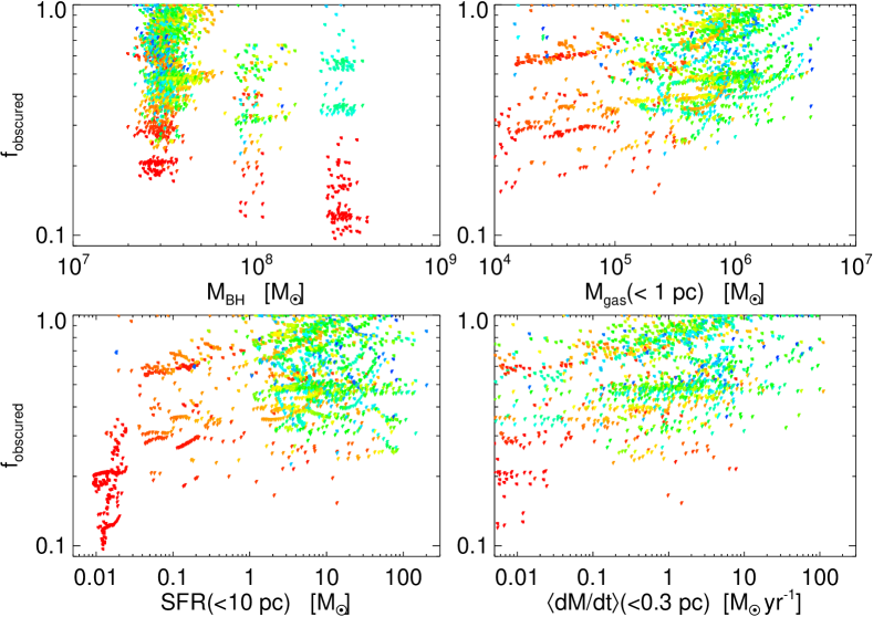
Figure 10: Obscured fraction (fraction of sightlines that encounter a column density $N_{\rm H}>10^{22}\,{\rm cm^{-2}}$) for our simulations as a function of various properties. Each simulation is sampled at several random times both before, during, and after its period of peak activity, and we show results from all simulations with different initial conditions and $q_{\rm eos}$ values. Points are colored by the instantaneous gas fraction inside of $10\,$pc (from red at $f_{\rm gas}<0.05$ to dark blue at $f_{\rm gas}>0.8$). Top Left: Versus $M_{\rm BH}$ (we add $\sim 0.1\,$dex scatter in $M_{\rm BH}$ so the points can be distinguished). For otherwise the same conditions (e.g. $M_{\rm gas}$), $f_{\rm obscured}$ declines with $M_{\rm BH}$ as approximately $\propto M_{\rm BH}^{-1/2}$. Top Right: Versus $M_{\rm gas}$ inside $1\,$pc, at fixed $M_{\rm BH}$. Obscured fractions increase weakly ($\propto M_{\rm gas}^{1/4}$) with gas mass. Bottom Left: Versus the star formation rate inside $10\,$pc. There is a weak increase in $f_{\rm obscured}$ with the circum-nuclear star formation rate, driven by the dependence on $M_{\rm gas}$ (slightly weaker $\propto\dot{M}_{\ast}^{0.15-0.2}$, because $\dot{M}_{\ast}^{0.15-0.2}$ is super-linear in $M_{\rm gas}$). Bottom Right: Versus inflow rate into small radii, at fixed $M_{\rm BH}=3\times 10^{7}\,M_{\sun}$ (if this continued to arbitrarily small radii, this would be proportional to the Eddington ratio $\dot{M}_{\rm BH}/\dot{M}_{\rm Edd}=L/L_{\rm Edd}$). The dependence here is significant, but very weak ($\propto\dot{M}^{0.1}$).

Figure 10 compares the obscured fraction in the “clumpy” model with a number of nuclear properties. For each simulation, we measure the relevant properties at randomly sampled times and viewing angles. We show the obscuration versus total mass inside some small radius (essentially, the BH mass), versus gas mass, versus the nuclear SFR, and versus the BH Eddington ratio.

Unsurprisingly, $f_{\rm obsc}$ increases with the gas mass inside a small radius $<1\,$pc. Note, however, that the correlation is weak: $f_{\rm obsc}\propto M_{\rm gas}^{1/4}$. The midplane columns should increase more rapidly with $M_{\rm gas}$, but these are already optically thick – the obscured fraction grows slowly with the fraction of sightlines above the disk that (at higher column) become optically thick. More interesting is the correlation this implies – $f_{\rm obsc}$ also increases with the nuclear SFR. Behavior along these lines has been observed at a wide variety of scales – Type 2 AGN are more likely to be found in more rapidly star-forming hosts, and/or hosts with younger stellar populations (Brotherton et al., 1999; Canalizo & Stockton, 2001; Yip et al., 2004; Jahnke et al., 2004; Zakamska et al., 2006; Nandra et al., 2007; Silverman et al., 2008). The observational correlation appears to be particularly strong when the nuclear stellar populations are isolated (Shi et al., 2007; Wang et al., 2007; Imanishi, 2002; Imanishi & Wada, 2004; Davies et al., 2007). Note that the SFRs inside of $\sim 10\,$pc can reach large $\sim 10\,M_{\sun}\,{\rm yr}$ values; however, as shown in Hopkins & Quataert (2010a) (Fig. 14), this is correlated with the BH inflow rates on these scales as $\dot{M}_{\ast}\sim\dot{M}_{\rm BH}$ (again, both tracing the gas mass supply) – for a less extreme quasar the “zero point” expected inside $\sim 10\,$pc would be more like $\sim 0.1-1\,M_{\sun}\,{\rm yr^{-1}}$. Conversely, ULIRGs and mergers with more pronounced star formation in their nuclei are more likely to host obscured Seyferts or quasars, whereas those with slightly older populations are more likely to exhibit Type 1 signatures (Farrah et al., 2003, 2005; Sanders, 1999; Guyon et al., 2006; Dasyra et al., 2006; Yuan et al., 2010).

Most likely, at least some of this trend owes to the role of AGN feedback in clearing away some of the gas and dust (see e.g. Sanders et al., 1988a; Hopkins et al., 2005c, b; Hopkins, 2011; Granato et al., 2004; Narayanan et al., 2006), but it can simply arise as we see here from the larger gas and dust supply “burying” the AGN until star formation exhausts much of that material. We stress that this is a true nuclear-scale ($<10\,$pc) correlation here, and the nuclear SF contributes negligibly ($\lesssim 0.3\,\%$) to the total SFR; there is not necessarily any predicted correlation between the AGN obscuration and the total/large-scale galaxy SFR.

Given similar gas properties, the obscured fraction decreases with BH mass. This is expected because the BH gravity provides a stabilizing force that tries to “flatten” the torus (for fixed gas properties, the disk $h/R\propto M_{\rm BH}^{-1/2}$). If more luminous AGN are, on average, more massive BHs, then this suggests an inverse correlation between QSO luminosity and obscured fractions. Indeed, the existence of such an apparent correlation is well-established (Hill et al., 1996; Simpson et al., 1999; Willott et al., 2000; Simpson & Rawlings, 2000; Steffen et al., 2003; Ueda et al., 2003; Grimes et al., 2004; Hasinger, 2004; Sazonov & Revnivtsev, 2004; Barger & Cowie, 2005; Simpson, 2005; Hao et al., 2005; Gilli et al., 2007; Hickox et al., 2007; Hasinger, 2008). However, it is still unclear precisely how much of this correlation owes to alternative possibilities such as simple dilution by the host galaxy and/or differences in the Eddington ratio distribution and accretion state (for a detailed discussion, see Hopkins et al., 2009b, and references therein). Moreover, without a full cosmological model to predict e.g. the distribution of active BH masses and Eddington ratios, we cannot forward model the BH luminosity distribution to construct a direct comparison with observations. But the predicted scaling here is not especially strong; it may well be that additional physics is needed to recover the full observed correlation – most commonly, AGN feedback is invoked to “blow away” some of the torus in the most luminous systems (see references above).

8 Discussion

We have studied AGN obscuration in a series of multi-scale hydrodynamic simulations that can self-consistently follow gas from $>10\,$kpc galactic scales to $<0.1\,$pc. These simulations include the full self-gravity of stars and gas (along with BHs and dark matter), gas cooling, and star formation, along with varied prescriptions for feedback from young stars; these are all critical to the behavior we see, and have not before been simultaneously modeled on nuclear scales. In these simulations, inflows from large scales, when sufficiently large, lead to a cascade of instabilities on small scales, ultimately yielding large nuclear gas masses and accretion rates onto the AGN. The scenario is qualitatively similar to the “bars within bars” model, but there is a high degree of variability and morphological diversity at each stage (with spirals, bars, clumps, flocculent structures, all present and alternatively powering inflows and outflows) – a more apt description would be “stuff within stuff” (Hopkins & Quataert, 2010a). Once gas nears the radius of influence of the BH, it generically forms an unstable $m=1$ mode (a lopsided or eccentric disk) that slowly precesses about the BH (Hopkins & Quataert, 2010b). The stellar and gas disk precess differently, leading to strong gravitational torques that can drive accretion rates of up to $\sim 10\,M_{\sun}\,{\rm yr^{-1}}$ onto the BH.

In this paper, we show that these nuclear, lopsided disks in fact naturally account for the long-invoked “toroidal obscuring region” used to explain the obscuration of Type 2 AGN. Up to now, these models have been essentially phenomenological – we show for the first time the formation of sub-pc scale obscuring structures from galaxy-scale inflows, and in a suite of $\sim 100$ simulations show that they are quite generic and arise ubiquitously with this inflow scenario. We show that the global dynamical properties – gas and stellar densities, density profiles, kinematics, gas fractions, and star formation rates, agree well with observations of AGN obscuring regions from scales as small as $0.1\,$pc to $\gtrsim 100\,$pc.

This implies a fundamentally new paradigm in which to view the obscuring region or “torus.” Far from being a passive bystander or simple fuel reservoir for the accretion process, it is itself the driver of that accretion. The torus is the gravitational structure on scales within the BH radius of influence that torques the gas and forces continuous gas inflow onto the BH. The same lopsided modes that drive accretion can also provide the scale height, column density distribution, and characteristic gas properties of the structure.

As such, the predicted torii have non-trivial substructure: both small-scale clumping in the gas (discussed below), global $m=1$ patterns, and warps/twists arising from bending modes at a range of radii. On large scales, the $m=1$ modes tend to manifest as lopsided/eccentric disks, or one-armed spirals; on small scales, they become more tightly wound spirals. Their typical amplitude in surface density is expected to be at the $\sim 10$’s of percent level (see Hopkins & Quataert, 2010a); the amplitude of induced non-circular velocities and corresponding magnitude of “offsets” of the BH from the spatial center of the galaxy nuclei (in units of the BH radius of influence) are about the same. Maser observations may show indications of asymmetry in the structure around nuclei (Schinnerer et al., 2000; Greenhill et al., 2003; Kondratko et al., 2005; Fruscione et al., 2005; Kondratko et al., 2006a); it is also possible that measurements of the velocity structure of e.g. molecular emission lines from the torus region may be able to measure such asymmetries in the near future.

We have argued that a large number of obscuration properties traditionally associated with “feedback” processes from AGN and star formation may, in fact, be explained by purely gravitational physics. Even in the absence of feedback, properly including the full self-gravity of gas and stars leads to disks with large $h/R$, sufficient to account for the observed column density distribution. This arises because of a combination of large-scale warps and twists (for example, where the lopsided disk mode meets an outer bar) and bending modes within the disk itself. The latter will, even in the absence of any large-scale twists or warps, tend to pump up $h/R$ wherever the eccentric disk mode is excited until an order unity $h/R\sim|a|$ is reached. Since bending modes are fast modes (pattern speed $\sim\Omega$), this can continuously transfer energy from the orbital motion to vertical motions on a single dynamical time, maintaining vertical scale heights even when the cooling time is arbitrarily short.

These warps and twists also naturally lead to the observed lack of correlation between nuclear-scale disk inclination angles and those of their parent/host galaxies. This will be even more prominent in systems which are driven on large scales by mergers, but can occur even in entirely secularly fueled AGN. They also account for observed gas velocity dispersions in AGN nuclei, and the correlations between those dispersions and quantities such as the local gas mass, star formation rate, and mass in young stars (all via their inherent dynamical correlations, not via any feedback channel). The efficiency of gravitational torques and induced inflow also naturally leads to convergence in nuclear gas masses and density profiles, leaving relic “cusps” similar to those observed (Hopkins & Quataert, 2011b).

These mechanisms can naturally explain observed global quantities such as the gas scale heights, masses, and density profiles. However, modeling the actual obscured fraction of AGN requires a more explicit model for the actual sub-structure on Jeans mass scales and well below, in the ISM surrounding black holes. We show in fact that any model which matches the observed dynamical properties (particularly global gas masses), but assumes “smooth” gas (uniformly distributed, say, out to some scale height corresponding to the average obscured fraction), will simultaneously fail to explain the observed column density distributions. A natural explanation for this discrepancy is that the gas is clumpy on multiple scales, broadening the column density distribution along all sightlines. There must, in fact, be structure on the relevant scales, since we know there is star formation at these radii (so some gas must reside in dense, tidally bound star-forming clumps). Unfortunately, our present models do not explicitly resolve the necessary physics of star formation and GMC formation/destruction via stellar feedback needed in order to explicitly simulate the sub-structure of the gas down to these scales.

However, we find that we can obtain predicted column density distributions in good agreement with those observed if we assume that whatever sub-grid clumps exist obey a couple of basic assumptions: namely that they are (at least at the order-of-magnitude level) near both virial and pressure equilibrium (or, instead of pressure equilibrium, that they are Jeans-scale in a $Q\sim 1$ self-regulating disk). These assumptions are sufficient to (statistically) predict the column density distribution that would be observed, regardless of the actual clump mass spectrum and physical origin (and without any adjustable parameter introduced). The predictions agree quite well with the column density distribution of both un-obscured, obscured, and Compton-thick AGN. This suggests that these basic properties should still hold for substructure in these regions, and that – if so – the uncertain quantities in our simulations (such as the feedback prescription and star formation recipe), make no dramatic difference in the column density distribution, since its key properties are set by the basic dynamics above. Essentially, if these assumptions hold, the distribution of observed column densities towards AGN is itself a natural consequence of gravitational clumping at the Jeans length/mass in a self-gravitating, globally $Q\sim 1$ disk – no exotic wind physics (driven by either stars or AGN) need to necessarily be invoked.

Higher-order probes of the structure in this region, for example studying the clump properties (their sizes and masses), constraining the ratio of stellar feedback to dynamical support in driving scale heights, and making predictions for line structure and other effects that might be used to probe the sub-structure and lopsided precession that power accretion, will require detailed treatment of the radiative transfer from the accretion disk through the circumnuclear region. This will be the subject of a future paper, and should enable a host of new predictions for comparison with future observations.

Another important next step will be the inclusion of realistic, physically motivated feedback models. Coupling our simulations with radiative transfer will be a major advance. Although this approach will not be strictly self-consistent, we will, for the first time, be able to examine how radiation pressure impacts inflowing and star-forming gas using a realistic description of multi-scale AGN gas distributions from $\sim 0.1-1000\,$pc scales. In particular, to study where the photon momentum is absorbed (compare Murray et al., 2005; Ciotti et al., 2010; Hopkins et al., 2011a), how radiation pressure profiles vary throughout the gas, how photon diffusion may affect the role of feedback (Thompson et al., 2005), and whether a realistic clumpy gas medium suppresses or enhances the efficiency of feedback-induced “shutdown” in star formation (Hall et al., 2007; Hopkins & Elvis, 2010; Tortora et al., 2009). In bright quasars and/or nuclear starbursts, the gas structure may well be modified not just locally (in terms of its clumpiness or sub-grid pressure support), but globally by strong outflows driven, for example, by radiation pressure (see Debuhr et al., 2011, and references therein). Even in the regime where some material is being expelled at the escape velocity, it is difficult to alter many of the basic dynamical properties of the gas (total mass enclosed and its relation to inflow rates, obscured fractions, etc) at the order-of-magnitude level (see e.g. Marconi et al., 2008), but may well make a large contribution to the observed scale height of obscuring material and can be critical to understanding how AGN self-regulate, why torii exhibit complex sub-structure, and perhaps scalings of obscured fraction with luminosity and/or redshift.

We have focused here on small-scale obscuration, at radii traditionally associated with the AGN “torus.” We stress, however, that this does not mean that there is a single object that accounts for the obscuration of all systems. As is evident in all of our comparisons, the gas distribution is truly continuous. Of course, there will be gas on small scales near the BH whenever it is active, which can occult and obscure different emission regions. This may take the form of an AGN wind, especially in high Eddington ratio systems (see e.g. Elvis, 2000; Elitzur & Shlosman, 2006).

There is also well-resolved gas from the host galaxies in these systems. The latter, on say $>100\,$pc scales, is not likely to be Compton-thick, simply because the characteristic Jeans scales, etc. are too large. However, this can easily dominate the production of more moderate column densities $N_{\rm H}\sim 10^{22}\,{\rm cm^{-2}}$. This “host galaxy obscuration” is especially important in the early phases of inflow forming a kpc-scale starburst, as the central kpc may be isotropically enshrouded in dust for a time $\sim 10^{8}\,$yr. Such obscuration as it arises in simulations of galaxy mergers has been discussed at length in e.g. Hopkins et al. (2005b, 2006a); Hopkins & Hernquist (2006); Hayward et al. (2011), and we refer to those papers for more details. Observations have also made it clear that a significant fraction of obscuration must come from host galaxies (especially in starbursts and edge-on disks; see e.g. Zakamska et al., 2006; Rigby et al., 2006; Martinez-Sansigre et al., 2009; Lagos et al., 2011) Since our current simulations are the first to simultaneously resolve both the nuclear scales where very large columns arise, and the galaxy scales where more moderate but potentially more isotropic (or at least differently-oriented) columns can arise, it will be interesting to investigate the relative contributions to obscuration from different scales, as a function of evolutionary stage and galaxy/BH properties. Because the AGN spectrum changes as it moves through the inner obscuring regions, this will require a full treatment of radiative transfer, as described above.

References

- Alexander et al. (2005) Alexander, D. M., Bauer, F. E., Chapman, S. C., Smail, I., Blain, A. W., Brandt, W. N., & Ivison, R. J. 2005, ApJ, 632, 736
- Alexander et al. (2008) Alexander, D. M., et al. 2008, ApJ, 687, 835
- Aller & Richstone (2007) Aller, M. C., & Richstone, D. O. 2007, ApJ, 665, 120
- Andre et al. (1996) Andre, P., Ward-Thompson, D., & Motte, F. 1996, A&A, 314, 625
- Antonucci (1993) Antonucci, R. 1993, ARA&A, 31, 473
- Barger & Cowie (2005) Barger, A. J., & Cowie, L. L. 2005, ApJ, 635, 115
- Barnes & Hernquist (1996) Barnes, J. E., & Hernquist, L. 1996, ApJ, 471, 115
- Barnes & Hernquist (1991) Barnes, J. E., & Hernquist, L. E. 1991, ApJL, 370, L65
- Bender et al. (2005) Bender, R., et al. 2005, ApJ, 631, 280
- Blitz & Rosolowsky (2006) Blitz, L., & Rosolowsky, E. 2006, ApJ, 650, 933
- Bournaud et al. (2007) Bournaud, F., Elmegreen, B. G., & Elmegreen, D. M. 2007, The Astrophysical Journal, 670, 237
- Braatz et al. (2004) Braatz, J. A., Henkel, C., Greenhill, L. J., Moran, J. M., & Wilson, A. S. 2004, ApJL, 617, L29
- Brotherton et al. (1999) Brotherton, M. S., et al. 1999, ApJL, 520, L87
- Bryant & Scoville (1999) Bryant, P. M., & Scoville, N. Z. 1999, AJ, 117, 2632
- Burlon et al. (2011) Burlon, D., Ajello, M., Greiner, J., Comastri, A., Merloni, A., & Gehrels, N. 2011, ApJ, 728, 58
- Canalizo & Stockton (2001) Canalizo, G., & Stockton, A. 2001, ApJ, 555, 719
- Cattaneo et al. (2005) Cattaneo, A., Combes, F., Colombi, S., Bertin, E., & Melchior, A. 2005, MNRAS, 359, 1237
- Cattaneo et al. (2009) Cattaneo, A., et al. 2009, Nature, 460, 213
- Ciotti et al. (2010) Ciotti, L., Ostriker, J. P., & Proga, D. 2010, ApJ, 717, 708
- Comastri et al. (1995) Comastri, A., Setti, G., Zamorani, G., & Hasinger, G. 1995, A&A, 296, 1
- Combes et al. (2004) Combes, F., et al. 2004, A&A, 414, 857
- Cox et al. (2006) Cox, T. J., Dutta, S. N., Di Matteo, T., Hernquist, L., Hopkins, P. F., Robertson, B., & Springel, V. 2006, ApJ, 650, 791
- Crenshaw et al. (2000) Crenshaw, D. M., et al. 2000, AJ, 120, 1731
- Croton et al. (2006) Croton, D. J., et al. 2006, MNRAS, 365, 11
- Cuadra et al. (2009) Cuadra, J., Armitage, P. J., Alexander, R. D., & Begelman, M. C. 2009, MNRAS, 393, 1423
- Daddi et al. (2007) Daddi, E., et al. 2007, ApJ, 670, 173
- Dasyra et al. (2006) Dasyra, K. M., et al. 2006, New Astronomy Review, 50, 720
- Davies et al. (2007) Davies, R. I., Sánchez, F. M., Genzel, R., Tacconi, L. J., Hicks, E. K. S., Friedrich, S., & Sternberg, A. 2007, ApJ, 671, 1388
- Davies et al. (2006) Davies, R. I., et al. 2006, ApJ, 646, 754
- Debattista et al. (2006) Debattista, V. P., Ferreras, I., Pasquali, A., Seth, A., De Rijcke, S., & Morelli, L. 2006, ApJL, 651, L97
- Debuhr et al. (2011) Debuhr, J., Quataert, E., & Ma, C. 2011, MNRAS, 412, 1341
- Deo et al. (2009) Deo, R. P., Richards, G. T., Crenshaw, D. M., & Kraemer, S. B. 2009, ApJ, 705, 14
- Deo et al. (2011) Deo, R. P., Richards, G. T., Nikutta, R., Elitzur, M., Gallagher, S. C., Ivezic, Z., & Hines, D. 2011, ApJ, in press, arXiv:1101.2855
- Di Matteo et al. (2005) Di Matteo, T., Springel, V., & Hernquist, L. 2005, Nature, 433, 604
- Donley et al. (2005) Donley, J. L., Rieke, G. H., Rigby, J. R., & Pérez-González, P. G. 2005, ApJ, 634, 169
- Dotti et al. (2009) Dotti, M., Ruszkowski, M., Paredi, L., Colpi, M., Volonteri, M., & Haardt, F. 2009, MNRAS, 396, 1640
- Downes & Solomon (1998) Downes, D., & Solomon, P. M. 1998, ApJ, 507, 615
- El-Zant & Shlosman (2003) El-Zant, A. A., & Shlosman, I. 2003, ApJL, 595, L41
- Elitzur & Shlosman (2006) Elitzur, M., & Shlosman, I. 2006, ApJL, 648, L101
- Elvis (2000) Elvis, M. 2000, ApJ, 545, 63
- Englmaier & Shlosman (2004) Englmaier, P., & Shlosman, I. 2004, ApJL, 617, L115
- Escala (2007) Escala, A. 2007, ApJ, 671, 1264
- Farrah et al. (2003) Farrah, D., Afonso, J., Efstathiou, A., Rowan-Robinson, M., Fox, M., & Clements, D. 2003, MNRAS, 343, 585
- Farrah et al. (2005) Farrah, D., Surace, J. A., Veilleux, S., Sanders, D. B., & Vacca, W. D. 2005, ApJ, 626, 70
- Feoli & Mancini (2009) Feoli, A., & Mancini, L. 2009, ApJ, 703, 1502
- Ferrarese & Merritt (2000) Ferrarese, L., & Merritt, D. 2000, ApJL, 539, L9
- Förster Schreiber et al. (2006) Förster Schreiber, N. M., et al. 2006, ApJ, 645, 1062
- Fruscione et al. (2005) Fruscione, A., Greenhill, L. J., Filippenko, A. V., Moran, J. M., Herrnstein, J. R., & Galle, E. 2005, ApJ, 624, 103
- Fukuda et al. (2000) Fukuda, H., Habe, A., & Wada, K. 2000, ApJ, 529, 109
- Fuller & Myers (1992) Fuller, G. A., & Myers, P. C. 1992, ApJ, 384, 523
- Gallimore et al. (2006) Gallimore, J. F., Axon, D. J., O’Dea, C. P., Baum, S. A., & Pedlar, A. 2006, AJ, 132, 546
- García-Burillo et al. (2005) García-Burillo, S., Combes, F., Schinnerer, E., Boone, F., & Hunt, L. K. 2005, Astronomy and Astrophysics, 441, 1011
- Gebhardt et al. (2000) Gebhardt, K., et al. 2000, ApJL, 539, L13
- Georgakakis et al. (2009) Georgakakis, A., et al. 2009, eprint arXiv, 0904, 3747, accepted for publication in MNRAS
- Georgantopoulos & Georgakakis (2005) Georgantopoulos, I., & Georgakakis, A. 2005, MNRAS, 358, 131
- Gilli et al. (2007) Gilli, R., Comastri, A., & Hasinger, G. 2007, A&A, 463, 79
- Granato et al. (2004) Granato, G. L., De Zotti, G., Silva, L., Bressan, A., & Danese, L. 2004, ApJ, 600, 580
- Greenhill et al. (1997) Greenhill, L. J., Moran, J. M., & Herrnstein, J. R. 1997, ApJL, 481, L23+
- Greenhill et al. (2003) Greenhill, L. J., et al. 2003, ApJ, 590, 162
- Grimes et al. (2004) Grimes, J. A., Rawlings, S., & Willott, C. J. 2004, MNRAS, 349, 503
- Guainazzi et al. (2005) Guainazzi, M., Fabian, A. C., Iwasawa, K., Matt, G., & Fiore, F. 2005, MNRAS, 356, 295
- Guyon et al. (2006) Guyon, O., Sanders, D. B., & Stockton, A. 2006, ApJS, 166, 89
- Hall et al. (2007) Hall, P. B., Sadavoy, S. I., Hutsemekers, D., Everett, J. E., & Rafiee, A. 2007, ApJ, 665, 174
- Hao et al. (2005) Hao, L., et al. 2005, AJ, 129, 1795
- Hasinger (2004) Hasinger, G. 2004, Nuclear Physics B Proceedings Supplements, 132, 86
- Hasinger (2008) —. 2008, A&A, 490, 905
- Hasinger et al. (2005) Hasinger, G., Miyaji, T., & Schmidt, M. 2005, A&A, 441, 417
- Hatziminaoglou et al. (2009) Hatziminaoglou, E., Fritz, J., & Jarrett, T. 2009, MNRAS, accepted, arXiv:0907.2389 [astro-ph]
- Hayward et al. (2011) Hayward, C. C., Kereš, D., Jonsson, P., Narayanan, D., Cox, T. J., & Hernquist, L. 2011, ApJ, in press [arXiv:1101.0002]
- Heller et al. (2001) Heller, C., Shlosman, I., & Englmaier, P. 2001, The Astrophysical Journal, 553, 661
- Henkel et al. (2005) Henkel, C., Peck, A. B., Tarchi, A., Nagar, N. M., Braatz, J. A., Castangia, P., & Moscadelli, L. 2005, A&A, 436, 75
- Hernquist (1989) Hernquist, L. 1989, Nature, 340, 687
- Hickox et al. (2007) Hickox, R. C., et al. 2007, ApJ, 671, 1365
- Hicks et al. (2009) Hicks, E. K. S., Davies, R. I., Malkan, M. A., Genzel, R., Tacconi, L. J., Sánchez, F. M., & Sternberg, A. 2009, ApJ, 696, 448
- Hill et al. (1996) Hill, G. J., Goodrich, R. W., & Depoy, D. L. 1996, ApJ, 462, 163
- Hobbs et al. (2010) Hobbs, A., Nayakshin, S., Power, C., & King, A. 2010, MNRAS, in press, arXiv:1001.3883
- Hoenig & Kishimoto (2009) Hoenig, S. F., & Kishimoto, M. 2009, A&A, in press, arXiv:0909.4539
- Hopkins (2010) Hopkins, P. F. 2010, MNRAS, in press, arXiv:1009.4702 [astro-ph]
- Hopkins (2011) —. 2011, MNRAS, in press, arXiv:1101.4230
- Hopkins et al. (2008a) Hopkins, P. F., Cox, T. J., Kereš, D., & Hernquist, L. 2008a, ApJS, 175, 390
- Hopkins et al. (2009a) Hopkins, P. F., Cox, T. J., Younger, J. D., & Hernquist, L. 2009a, ApJ, 691, 1168
- Hopkins & Elvis (2010) Hopkins, P. F., & Elvis, M. 2010, MNRAS, 401, 7
- Hopkins & Hernquist (2006) Hopkins, P. F., & Hernquist, L. 2006, ApJS, 166, 1
- Hopkins & Hernquist (2010) —. 2010, MNRAS, 402, 985
- Hopkins et al. (2005a) Hopkins, P. F., Hernquist, L., Cox, T. J., Di Matteo, T., Martini, P., Robertson, B., & Springel, V. 2005a, ApJ, 630, 705
- Hopkins et al. (2005b) Hopkins, P. F., Hernquist, L., Cox, T. J., Di Matteo, T., Robertson, B., & Springel, V. 2005b, ApJ, 632, 81
- Hopkins et al. (2006a) —. 2006a, ApJS, 163, 1
- Hopkins et al. (2008b) Hopkins, P. F., Hernquist, L., Cox, T. J., & Kereš, D. 2008b, ApJS, 175, 356
- Hopkins et al. (2006b) Hopkins, P. F., Hernquist, L., Cox, T. J., Robertson, B., Di Matteo, T., & Springel, V. 2006b, ApJ, 639, 700
- Hopkins et al. (2007a) Hopkins, P. F., Hernquist, L., Cox, T. J., Robertson, B., & Krause, E. 2007a, ApJ, 669, 45
- Hopkins et al. (2007b) —. 2007b, ApJ, 669, 67
- Hopkins et al. (2006c) Hopkins, P. F., Hernquist, L., Cox, T. J., Robertson, B., & Springel, V. 2006c, ApJS, 163, 50
- Hopkins et al. (2005c) Hopkins, P. F., Hernquist, L., Martini, P., Cox, T. J., Robertson, B., Di Matteo, T., & Springel, V. 2005c, ApJL, 625, L71
- Hopkins et al. (2009b) Hopkins, P. F., Hickox, R., Quataert, E., & Hernquist, L. 2009b, MNRAS, 398, 333
- Hopkins et al. (2006d) Hopkins, P. F., Narayan, R., & Hernquist, L. 2006d, ApJ, 643, 641