New code for equilibriums and quasiequilibrium initial data of compact objects

Abstract

We present a new code, named COCAL - Compact Object CALculator, for the computation of equilibriums and quasiequilibrium initial data sets of single or binary compact objects of all kinds. In the cocal code, those solutions are calculated on one or multiple spherical coordinate patches covering the initial hypersurface up to the asymptotic region. The numerical method used to solve field equations written in elliptic form is an adaptation of self-consistent field iterations in which Green’s integral formula is computed using multipole expansions and standard finite difference schemes. We extended the method so that it can be used on a computational domain with excised regions for a black hole and a binary companion. Green’s functions are constructed for various types of boundary conditions imposed at the surface of the excised regions for black holes. The numerical methods used in cocal are chosen to make the code simpler than any other recent initial data codes, accepting the second order accuracy for the finite difference schemes. We perform convergence tests for time symmetric single black hole data on a single coordinate patch, and binary black hole data on multiple patches. Then, we apply the code to obtain spatially conformally flat binary black hole initial data using boundary conditions including the one based on the existence of equilibrium apparent horizons.

I Introduction

In the last decades, simulation codes for compact objects have been successfully developed in the field of numerical relativity, and various dynamical simulations have been performed including binary neutron stars and black holes inspirals to merger NRreview , a massive core-collapse to a proto neutron star or a black hole (BH) formation SN , and black hole dynamics HigherDimBH . Recent efforts on these subjects are, for example, to study more realistic situations by including microphysics of the neutron stars (NS) RecentNS , wider range of parameter space such as mass ratio and spins of binary black hole (BBH) mergersRecentBH or BBH mergers in an ambient disk RecentBBH . Accordingly, more realistic and accurate construction of initial data for such compact objects is required.

Several researchers have developed methods for computing various types of initial data sets for those simulations Cook:2000vr ; BBH_QE ; BNSCF ; BHNS_QE ; UryuCF ; UryuWL ; TU2007 ; Huang:2008vp , and equilibriums of rotating compact objects (see e.g. RNSreview ). Many of such initial data codes are specialized to a certain problem such as a single stationary and axisymmetric neutron star or BBH data on a conformally flat initial hypersurface. An exception is lorene lorene , which is one of most used code for computing initial data for the merger simulations of binary neutron stars and black holes. The lorene code was originally developed for computing rapidly rotating neutron stars, but has been extended to be capable of computing various kinds of equilibriums and quasiequilibrium initial data sets.

In this paper, we introduce our project for developing new codes for computing initial data of astrophysical compact objects, a single as well as binary compact objects of all kinds, and present several tests for the new codes. Our aim is to develop a set of codes for computing, on an initial hypersurface, a single neutron star (or a compact star such as a quark star), binary neutron stars and black holes, a central neutron star or black hole surrounded by a toroidal disk, and all these systems with magnetic fields. We call our new codes “cocal” as the abbreviation for Compact Object CALculator . A noteworthy idea of the “cocal” project is to develop a code using less technical numerical methods than the recent initial data solvers with spectral methods BBH_QE ; BNSCF ; BHNS_QE ; lorene . Also the modules and subroutines of the fortran90 code are structured simply so that the code may be accessible by those who mastered introductory courses for programing. Such feature will help future developments to incorporate more complex physics in the code such as radiation, neutrino radiation transfers, or realistic equations of state for the high density nuclear matter.

The numerical method used in cocal is based on Komatsu-Eriguchi-Hachisu (KEH) method for computing equilibrium of a rotating neutron star KEH89 . In our previous works UryuCF ; UryuWL , we have extended KEH method for computing initial data for binary compact objects in quasiequilibriums. Among all, in the paper TU2007 , we have introduced multiple spherical coordinate patches for computing binary compact objects. We improve the idea of the multiple patches in all aspects in the new cocal code. In the paper Huang:2008vp , we have presented convergence tests and solution sequences for rotating neutron star initial data, which was calculated by the first version of cocal. In this paper for introducing the cocal code, we focus on the basic setup of the multiple spherical coordinate patches and the coordinate grids, the method of elliptic equation solver on the multiple patches, and convergence tests for binary black hole initial data. The paper is organized as follows: in Sec.II, we introduce an overview of the cocal project, then coordinate setups, elliptic solver and other materials on numerical computing. In Sec.III the results of convergence tests are presented. In Sec.IV solutions of BBH data on a conformally flat initial hypersurface are presented. We use geometric units with $G=c=1$ throughout the paper.

II COCAL code

II.1 Overview

In the cocal project, we aim to develop numerical codes for computing a single compact object as well as binary compact objects in (quasi)equilibrium using common numerical method as much as possible. A plan for such codes also depends on how to formulate the problem to solve such compact objects. Usually, a system of equations to describe equilibrium systems of compact objects involves a set of elliptic equations for the gravitational fields, and relativistic hydrodynamical equations including Euler equation and the rest mass conservation equation, to which a stationary condition, either a time or a helical symmetry Friedman:2001pf , is imposed. When the magnetic field is present, elliptic equations for the electromagnetic fields are added, and the equations for the fluid is replaced by magnetohydrodynamical (MHD) Euler equation. Because the stationary Euler, or MHD-Euler, equations are difficult to integrate numerically, a set of the first integrals in the form of algebraic equations, a sufficient condition for the stationary (MHD) Euler equations, is derived and solved simultaneously with the field equations (see e.g. Uryu:2010su ; Gourgoulhon:2011gz ).

A choice of a numerical method is therefore made according to what kind of solver is used for solving the system of elliptic equations. The numerical method used in cocal is based on KEH method for computing equilibriums of rotating neutron stars KEH89 . In this method, the elliptic equations are solved on spherical coordinates using the Green’s formula iteratively. This is done by separating the flat Laplacian or Helmholtz operator on the variable to be solved for, then moving remaining (possibly non-linear) terms to the source, and rewriting it in the integral form using Green’s formula. Expanding the Green’s function using spherical harmonics, the formula is integrated on the spherical coordinate grids numerically (see, e.g. UryuCF ; UryuWL ; YBRUF06 ). The method is extended for computations of binary compact objects as discussed in this section.

We choose simple finite difference formulas which are mostly second order accurate, and in some cases choose third or fourth order formulas only if they are necessary (see Sec. III.2.1). No symmetry, such as an equatorial plane symmetry, is assumed a priori on the 3D spherical computational domain. The cocal code is written in Fortran 90 language, and runs with a few GB of memory for a model with a moderate resolution.

We have developed basic subroutines for the cocal code, including the coordinate grid setups for a single and multiple spherical coordinates, as well as the elliptic solvers for a single or binary compact objects, which we discuss in detail below. Mainly, two types of initial value formulation for Einstein’s equation have been coded so far; one is assuming spatial conformal flatness (Isenberg-Wilson-Mathews formulation ISEN78 ; WM89 ), and the other non-conformal flatness (waveless formulation SUF04 ; UryuWL ).

Also, the quadrupole formula to compute the gravitational wave amplitude and luminosity, and a Helmholtz solver have been developed. We are in the phase to test all basic subroutines by computing simple test problems as well as known problems such as BBH initial data, or rotating neutron star solutions. In the next step, we will combine these developments and start computing new equilibriums and initial data sets such as helically symmetric binary compact objects, or magnetized compact objects.

II.2 Coordinate patches for binary systems

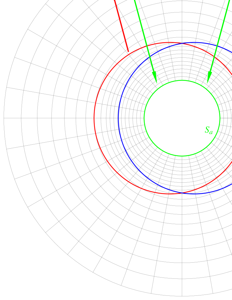
Figure 1: A typical setup for multiple coordinate grid patches in the cocal code for a BH-NS system. Left and right top patches are those for compact object coordinate patches (COCP) centered at each compact object (BH for the left, and NS for the right). The smallest circle with thick curve in COCP-BH is the sphere $S_{a}$ where the interior region is excised and certain BH boundary conditions are imposed. The ovals drawn in COCP-NS denote NS. Bottom patch is that for asymptotic region coordinate patch (ARCP), centered at the mass center of the system, and extends to asymptotics. The arrows represent maps of potentials between the multiple patches. Alternatively, the radius of COCP may be extended to asymptotics, instead of using ARCP. Note that the spheres $S_{a}$, $S_{b}$, and $S_{e}$ of these coordinate patches are distinct ones on a spacelike hypersurface $\Sigma_{t}$. The radius of each coordinate patch doesn’t reflect the size used in actual computations.

We assume that the spacetime is $\cal M$ is foliated by a family of spacelike hypersurface $(\Sigma_{t})_{t\in{\mathbb{R}}}$, ${\cal M}={\mathbb{R}}\times\Sigma$ parametrized by $t\in{\mathbb{R}}$. In the cocal code, we solve fields on a initial hypersurface $\Sigma_{t}$ which may be stationary (in equilibrium), or quasi-stationary (in quasi-equilibrium). The initial hypersurface $\Sigma_{t}$ is covered by overlapping multiple spherical coordinate patches whose coordinates are denoted by $(r,\theta,\phi)$. Angular coordinates cover all directions $(\theta,\phi)\in[0,\pi]\times[0,2\pi]$ without any symmetry imposed. We also introduce Cartesian coordinates as a convenient reference frame in a standard manner, that is, to have the positive side of x-axis coincide with a $(\theta,\phi)=(\pi/2,0)$ line, that of y-axis with a $(\theta,\phi)=(\pi/2,\pi/2)$ line, and that of z-axis with a $\theta=0$ line.

In Fig. 1, a schematic figure of three spherical coordinate patches whose coordinates are discretized in grid points is shown for the case of computing BH-NS binary systems by cocal. Shown is the 2D section of the 3D hypersurface, that may agree with the equatorial or meridional plane of the compact objects. Even though this may be the most complex setup for coordinate grids in cocal, it is not technical at all compared to those of existing codes in which adaptive coordinates are used.

For the computation of binary systems, two compact objects are placed at the centers of the two patches. We call these two patches the compact object coordinate patch (COCP), and the third patch the asymptotic region coordinate patch (ARCP). A domain of COCP is defined between two concentric spheres $S_{a}$ and $S_{b}$ from which an interior of an another sphere $S_{e}$ is excised. Writing radii of $S_{a}$, $S_{b}$, and $S_{e}$ as $r_{a}$, $r_{b}$, and $r_{e}$ respectively, we define spherical coordinates of COCP as $(r,\theta,\phi)\in[r_{a},r_{b}]\times[0,\pi]\times[0,2\pi]$, and locate the center of the excised sphere at $(r,\theta,\phi)=(d_{s},\pi/2,0)$, that is on the positive side of the x-axis . We introduce the excision of a domain interior of the sphere $S_{e}$ for computing binary systems, and elucidate its role in the following section. When a single and/or axisymmetric object is computed, the excision inside $S_{e}$ is not used. When BH is computed on COCP-BH with certain BH boundary conditions on $S_{a}$ $(r_{a}>0)$, the region inside of $S_{a}$ is excised. When a NS or a puncture BH is calculated, the sphere $S_{a}$ of COCP is removed by setting $r_{a}=0$, so the radial coordinate covers up to $r=0$. A domain of ARCP is defined between two concentric spheres $S_{a}$ and $S_{b}$, and its spherical coordinates are defined as $(r,\theta,\phi)\in[r_{a},r_{b}]\times[0,\pi]\times[0,2\pi]$. When values of field potentials or other variables are communicated from one patch to the other, those values on a certain sphere are mapped to a corresponding boundary sphere as indicated by arrows in Fig. 1.

Values of radii $r_{a}$, $r_{b}$, and $r_{e}$ for each of the coordinate patches used in actual computations will be summarized in Sec. III. Typically, they are set as follows. For the case of using three patches as in Fig. 1, the radius $r_{a}$ of the inner boundary $S_{a}$ of ARCP is taken large enough to be placed outside of the excised spheres $S_{e}$ for compact objects on COCP, but small compare to the size of the domain $r_{b}$ of the COCP. The outer boundary of ARCP, the radius $r_{b}$ of the sphere $S_{b}$, is extended to the asymptotic region when a field to be calculated behaves as a Coulomb type fall off, while it is truncated at the near zone when a radiation field is calculated. The center of ARCP is located at the center of mass of binary compact objects. Therefore typically, for compact objects with a mass $M$, $r_{a}={O}(M)$ (0 for NS), $r_{b}={O}(100M)$, and $r_{e}={O}(M)-{O}(10M)$ for COCP, and $r_{a}={O}(10M)$, and $r_{b}={O}(10^{6}M)$ or larger for ARCP.

As an another option for the choice of coordinate patch, the outer radius of each COCP $r_{b}$ may be extended to asymptotics, say $r_{b}={O}(10^{6}M)$, and ARCP is removed. This option simplifies the code, but it can not be used when a radiation field is computed by solving Helmholtz equation. We present tests for the Helmholtz solver in a separate paper.

II.3 Elliptic equation solver

As mentioned earlier, the formulation for computing (quasi-)equilibrium configurations of compact objects results in a coupled system of elliptic equations, either Poisson or Helmholtz equations with non-linear source terms, coupled with algebraic equations. The numerical method used in cocal to solve such a system of equations is an extension of KEH method which is an application of self-consistent field method for computing equilibriums of self-gravitating fluids to general relativistic stars KEH89 . A distinctive feature of these methods is the use of Green’s formula for an elliptic equation solver. We have introduced in previous papers our implementation of KEH method to compute binary neutron stars and black holes TU2007 ; Huang:2008vp ; UryuCF ; UryuWL .

In the cocal code, we have made a major change in the choice of coordinate patch, and accordingly in the elliptic equation solver. Our new implementation is better in all aspects for computing binary compact objects than our previous ones. We come back to discuss this point after we introduce the elliptic equation solver in cocal.

In solving each field equation, we separate out a flat Laplacian or Helmholtz operator $\cal L$, and write it with a non-linear source S,

$${\cal L}\Phi=S,$$ (1)

on an initial slice $\Sigma_{t}$, where $\Phi$ represents metric potentials. For the case of Laplacian ${\cal L}=\Delta$, using the Green’s function without boundary $G(x,x^{\prime})=1/|x-x^{\prime}|$ that satisfies

$$\Delta G(x,x^{\prime})=-4\pi\delta(x-x^{\prime}),$$ (2)

Green’s identity is obtained by

$$\Phi(x)=-\frac{1}{4\pi}\int_{V}G(x,x^{\prime})S(x^{\prime})d^{3}x^{\prime}\qquad\qquad\qquad$$

$$+\frac{1}{4\pi}\int_{\partial V}\left[G(x,x^{\prime})\nabla^{\prime a}\Phi(x^{\prime})-\Phi(x^{\prime})\nabla^{\prime a}G(x,x^{\prime})\right]dS^{\prime}_{a}.\ \ \$$ (3)

where $V$ is the domain of integration, $x,x^{\prime}\in V\subseteq\Sigma_{0}$, and $\partial V$ is its boundary. For the case of BH-NS system shown in Fig. 1, the boundary of COCP-BH becomes $\partial V=S_{a}\cup S_{b}\cup S_{e}$, that of COCP-NS $\partial V=S_{b}\cup S_{e}$, and that of ARCP $\partial V=S_{a}\cup S_{b}$. For the evaluation of the integrals in Eq.(3), a multipole expansion of $G(x,x^{\prime})$ in associated Legendre functions on the spherical coordinate is used;

$$G(x,x^{\prime}) = \frac{1}{\left|{x}-{x^{\prime}}\right|}\,=\,\sum_{\ell=0}^{\infty}g_{\ell}(r,r^{\prime})\sum_{m=0}^{\ell}\epsilon_{m}\,\frac{(\ell-m)!}{(\ell+m)!}$$ (4)

$$\!\!\!\!\!\!\!\times P_{\ell}^{~{}m}(\cos\theta)\,P_{\ell}^{~{}m}(\cos\theta^{\prime})\cos m(\varphi-\varphi^{\prime}),$$

where the radial Green’s function $g_{\ell}(r,r^{\prime})$ is defined by

$$g_{\ell}(r,r^{\prime})=\frac{r_{<}^{\ell}}{r_{>}^{\ell+1}},$$ (5)

with $r_{>}:=\sup\{r,r^{\prime}\},\ r_{<}:=\inf\{r,r^{\prime}\},$ and the coefficients $\epsilon_{m}$ are equal to $\epsilon_{0}=1$, and $\epsilon_{m}=2$ for $m\geq 1$.

Eq.(3) is an integral identity but is not a solution of Eq.(1) in a sense that both of $\Phi$ and its derivative $n^{a}\nabla_{a}\Phi$ can not be specified freely. Eq. (3) can be used to compute a potential over $V$, only if correct values of $\Phi$ and $n^{a}\nabla_{a}\Phi$ are known at the boundary $\partial V$. Here, $n^{a}$ is an outward normal to $\partial V$. Therefore, as it is commonly found in standard text books for electromagnetism Jackson , a homogeneous function $F(x,x^{\prime})$ for the Laplacian is added to evaluate the Green’s function that satisfies the boundary condition at $\partial V$. For example, a Green’s function $G(x,x^{\prime})+F(x,x^{\prime})=0$ at $\partial V$ is used to impose Dirichlet boundary condition. In our previous paper TU2007 , we have developed an elliptic equation solver on multiple coordinate patches that uses such Green’s functions and solve Eq.(3) by iteration.

A construction of such a Green’s function that satisfies a boundary condition is, however, possible only when a certain specific geometry of the domain of computation is adapted to the coordinate systems. In the present case for COCP of the cocal code in Fig. 1, a Green’s function that satisfy boundary conditions at $S_{a}$ and $S_{b}$ may not be derived in a practical form of equation, because we excised the region inside of the sphere $S_{e}$. To impose boundary conditions at $S_{a}$ and $S_{b}$, we introduce a homogeneous solution $\chi(x)$, and write a formal solution as

$$\Phi(x)\,=\,\chi(x)\,+\,{\Phi_{\rm INT}}(x),$$ (6)

where ${\Phi_{\rm INT}}$ is equal to the right hand side of Eq.(3);

$${\Phi_{\rm INT}}(x)=-\frac{1}{4\pi}\int_{V}G(x,x^{\prime})S(x^{\prime})d^{3}x^{\prime}\qquad\qquad\qquad$$

$$+\frac{1}{4\pi}\int_{\partial V}\left[G(x,x^{\prime})\nabla^{\prime a}\Phi(x^{\prime})-\Phi(x^{\prime})\nabla^{\prime a}G(x,x^{\prime})\right]dS^{\prime}_{a}.\ \ \$$ (7)

The homogeneous solution is computed so that the potential $\Phi$ satisfies the boundary conditions, which are either one of Dirichlet, Neumann, or Robin boundary conditions at the boundary spheres $S_{a}$ or $S_{b}$;

$${\rm Dirichlet:}\quad \Phi_{\rm BC}\,=\,f_{\rm D}$$ (8)

$${\rm Neumann:}\quad n^{a}\nabla_{a}\Phi_{\rm BC}\,=\,f_{\rm N}$$ (9)

$${\rm Robin:}\quad n^{a}\nabla_{a}\Phi_{\rm BC}+\frac{1}{4}\nabla_{a}n^{a}\Phi_{\rm BC}\,=\,f_{\rm R}$$ (10)

where $f_{\rm D}$, $f_{\rm N}$, and $f_{\rm R}$ are given functions on the spheres $S_{a}$ or $S_{b}$. Formulas for $\chi(x)$ are derived by using a Legendre expansion in an usual manner as shown in Appendix. Noticing $\chi(x)=\Phi(x)\,-\,{\Phi_{\rm INT}}(x)$ the formulas for $\chi(x)$ can be written analogously to the surface integral terms of Green’s formula, but with a different kernel function $G^{\rm BC}$

$$\chi(x) = \frac{1}{4\pi}\int_{S_{a}\cup S_{b}}\left[G^{\rm BC}(x,x^{\prime})\nabla^{\prime a}(\Phi_{\rm BC}-{\Phi_{\rm INT}})(x^{\prime})\right.$$ (11)

$$\left.-(\Phi_{\rm BC}-{\Phi_{\rm INT}})(x^{\prime})\nabla^{\prime a}G^{\rm BC}(x,x^{\prime})\right]dS^{\prime}_{a}.$$

The function $G^{\rm BC}(x,x^{\prime})$ is expanded in terms of the associated Legendre functions

$$G^{\rm BC}(x,x^{\prime}) = \sum_{\ell=0}^{\infty}g^{\rm BC}_{\ell}(r,r^{\prime})\sum_{m=0}^{\ell}\epsilon_{m}\,\frac{(\ell-m)!}{(\ell+m)!}$$ (12)

$$\!\!\!\!\!\!\!\!\!\!\!\!\!\!\!\!\!\times P_{\ell}^{~{}m}(\cos\theta)\,P_{\ell}^{~{}m}(\cos\theta^{\prime})\cos m(\varphi-\varphi^{\prime}),$$

where the radial function $g^{\rm BC}_{\ell}(r,r^{\prime})$ is chosen according to the type of boundary conditions used. We derive such radial functions used in the corresponding surface integrals for various cases of boundary conditions as listed in Table 1. Concrete forms of these functions are presented in Appendix B.

$G^{\rm BC}(x,x^{\prime})$	Boundary $S_{a}$	Boundary $S_{b}$
$G^{\rm NB}(x,x^{\prime})$	None	None
$G^{\rm DD}(x,x^{\prime})$	Dirichlet	Dirichlet
$G^{\rm ND}(x,x^{\prime})$	Neumann	Dirichlet
$G^{\rm DN}(x,x^{\prime})$	Dirichlet	Neumann
$G^{\rm NN}(x,x^{\prime})$	Neumann	Neumann
$G^{\rm RD}(x,x^{\prime})$	Robin	Dirichlet
$G^{\rm DR}(x,x^{\prime})$	Dirichlet	Robin

Table 1: List of Green’s function available in the cocal code. The second and third columns correspond to the types of boundary conditions imposed on the boundary spheres $S_{a}$ and $S_{b}$, respectively. The case with no boundary condition is denoted by None.

II.4 Iteration procedure

The final solution will be obtained from the iteration of Eq. (6), with Eqs. (7) and (11), where explicit form of Eq. (11) for $\chi(x)$ depends on the boundary condition, for example, Eq. (47) or (50).

We summarize the $n^{\rm th}$ step of the Poisson solver in the cocal code as follows:

• Compute the volume source term $S(\Phi^{(n-1)})$ as well as the surface source terms on all possible surfaces $S_{a}$, $S_{b}$, $S_{e}$.

• Compute the volume integral and the surface integral at $S_{e}$ for obtaining $\widehat{\Phi}_{\rm INT}(x)$ from Eq. (7).

• Compute the effective source for the integral on $S_{a}$ and $S_{b}$. For Dirichlet boundary condition it will be $\Phi_{\rm BC}-\widehat{\Phi}_{\rm INT}$, while for Neumann $\frac{\partial\Phi_{\rm BC}}{\partial r}-\frac{\partial\widehat{\Phi}_{\rm INT}}{\partial r}$.

• Compute the surface integrals at $S_{a}$ and $S_{b}$ for obtaining $\widehat{\chi}(x)$ according to Eq. (11) using the appropriate function $G^{\rm BC}$ for the boundary conditions of the problem.

• Add the results from steps 2) and 4) to obtain $\widehat{\Phi}(x)$ from Eq. (6).

• Update $\Phi^{(n)}$ according to

  $$\Phi^{(n)}(x)\,:=\,c\widehat{\Phi}(x)+(1-c)\Phi^{(n-1)}(x)$$

  where $0.1\leq c\leq 0.4$.

• Check if

  $$2\frac{|\Phi^{(n)}-\Phi^{(n-1)}|}{|\Phi^{(n)}|+|\Phi^{(n-1)}|}<\epsilon_{c}$$

  for all points of the grids, where $\epsilon_{c}=10^{-6}-10^{-8}$ is taken in typical computations, and $\epsilon_{c}=10^{-7}$ in this paper. If yes exit. If no go back to step 1).

Here, intermediate variables during an iteration step are denoted with a hat as $\widehat{\Phi}_{\rm INT}$, $\widehat{\chi}$, and $\widehat{\Phi}$. The above iteration procedure is applied to each coordinate patch one after other. In step 1), the sources of the surface terms are computed either from boundary conditions to be imposed on the surface, or from data of corresponding surface on the other patch (see, Fig. 1 how the potentials are transferred from a boundary surface to the other). Several different iteration schemes are possible for solving a set of elliptic equations for more than one variable. As long as we experimented, a convergence of the iteration does not depend on the order of computing those variables at each iteration step.

We will see this elliptic equation solver produce accurate solutions for test problems of binary black hole data. Two comments on the elliptic equation solver are made here. Although, ${\Phi_{\rm INT}}$ in Eq. (7) involves surface integrals on all $S_{a}$, $S_{b}$, and $S_{e}$, those on $S_{a}$ and $S_{b}$ are not included in ${\Phi_{\rm INT}}$ in an actual computation. Those computations are redundant because the homogeneous solution $\chi(x)$ is determined again from the surface integrals on $S_{a}$ and $S_{b}$ as in Eq. (11). So far, we do not plan to develop elliptic solvers for vector (tensor) fields in which Green’s functions are expanded in vector (tensor) spherical harmonics. Instead, we write the Cartesian components of vector or tensor equations, and solve each components as scalar equations on spherical grids for simplicity. We will see an example in Sec. IV (see also, UryuWL ).

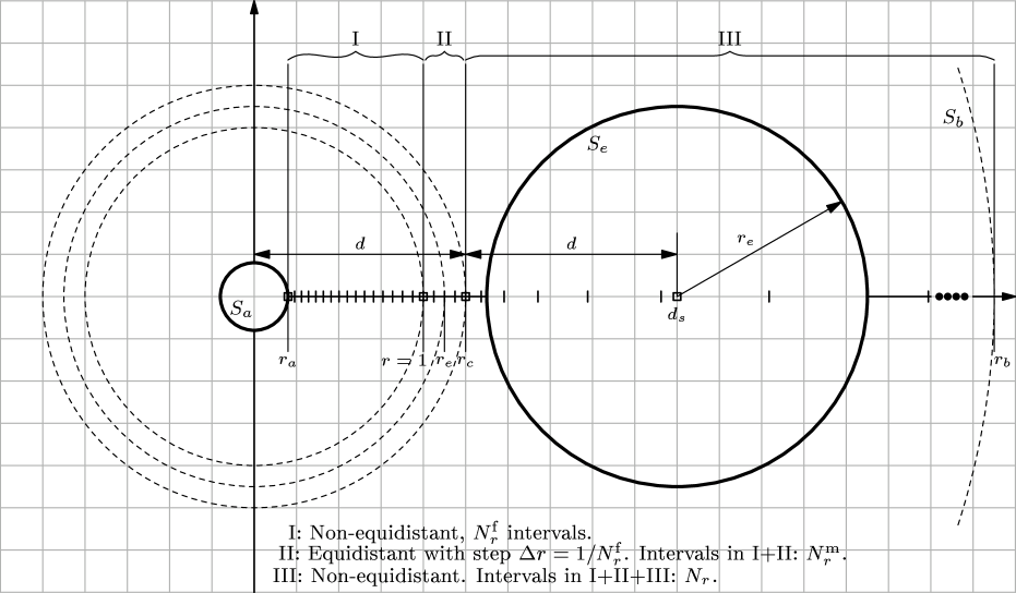
Figure 2: Radial coordinate grids for COCP for the case of regions for BH and binary companion being excised. The radial coordinate grids corresponds to those of lowest resolutions A1, B1, D1 and F1 in Tables 3 and 4.

II.5 Grid spacing

We apply finite difference scheme to solve the system of equations for compact objects on the spherical domain introduced in Sec II.2 (see, Fig. 1). Spherical coordinates $(r,\theta,\phi)$ for COCP and ARCP are bounded by two concentric spheres $S_{a}$ and $S_{b}$ of radius $r_{a}$ and $r_{b}$, respectively, with the possible excision of a sphere $S_{e}$ of radius $r_{e}$ inside COCP. The origin of the radial coordinate $r$ is placed at the common center of $S_{a}$ and $S_{b}$, where the compact object is placed for the case of COCP. Excised sphere for a binary companion $S_{e}$ is always positioned at a positive value on the x-axis at a distance $d_{s}$ from the origin. Clearly $r_{a}<d_{s}-r_{e}$. For neutron star calculations the sphere $S_{a}$ is absent and the coordinate system extends from $r=0$ to $r_{b}$.

In the cocal code, the spacing of all coordinate grid points $(r_{i},\theta_{j},\phi_{k})$ with $i=0,\cdots,N_{r}$, $j=0,\cdots,N_{\theta}$, and $k=0,\cdots,N_{\phi}$, are freely specifiable. However, in ($\theta,\phi$) directions, uniform grids are recommended to resolve the trigonometric and associated Legendre functions used in the elliptic equation solver, as well as a structure of compact objects evenly. That is, we set the grid interval in these directions as

$$\Delta\theta_{j} = \theta_{j}-\theta_{j-1}\,=\,\Delta\theta\,=\,\frac{\pi}{N_{\theta}},$$ (13)

$$\Delta\phi_{k} = \phi_{k}-\phi_{k-1}\,=\,\Delta\phi\,=\,\frac{2\pi}{N_{\phi}}.$$ (14)

The grid spacing in the radial direction $r$ is usually constructed on one hand to resolve the vicinity of the compact object with finer grid spacings, and on the other hand to extend to asypmtotics using increasingly sparse spacings. The setup for radial grids of COCP in the present computation is illustrated in Fig. 2. The grid is composed from three regions I, II, and III. For the case with $r_{a}<1$, the region I is set by $r\in[r_{a},1]$ the region II by $r\in[1,r_{c}]$, and region III $r\in[r_{c},r_{b}]$. We introduce grid numbers ${N_{r}^{\rm f}},\ {N_{r}^{\rm m}}$ which correspond to the numbers of intervals in regions I and I+II, respectively. We introduce a standard grid spacing $\Delta r$ as $\Delta r=1/{N_{r}^{\rm f}}$. For the case with $r_{a}<1$, the grid intervals, $\Delta r_{i}:=r_{i}-r_{i-1}$, are defined by

$$\Delta r_{i+1} = h\Delta r_{i},\ \ \mbox{for}\ \ i=1,\cdots,{N_{r}^{\rm f}}-1$$ (15)

$$\Delta r_{i\phantom{+1}} = \phantom{h}\Delta r,\ \ \ \mbox{for}\ \ i={N_{r}^{\rm f}},\cdots,{N_{r}^{\rm m}}$$ (16)

$$\Delta r_{i+1} = k\Delta r_{i},\ \ \mbox{for}\ \ i={N_{r}^{\rm m}},\cdots,N_{r}-1\ \$$ (17)

which correspond to regions I, II, and III in Fig. 2, respectively, where ratios $h(\leq 1)$ and $k(>1)$ are respectively determined from relations

$$1-r_{a} = \Delta r\frac{1-h^{N_{r}^{\rm f}}}{1-h},$$ (18)

$$r_{b}-r_{c} = \Delta r\frac{k(k^{N_{r}-{N_{r}^{\rm m}}}-1)}{k-1}.$$ (19)

For the case with $r_{a}>1$, which is mostly for ARCP, the grid intervals, $\Delta r_{i}$, are defined by

$$\Delta r_{i} = \phantom{h}\Delta r\ \ \ \mbox{for}\ \ i=1,\cdots,{N_{r}^{\rm m}},$$ (20)

$$\Delta r_{i+1} = k\Delta r_{i}\ \ \mbox{for}\ \ i={N_{r}^{\rm m}},\cdots,N_{r}-1,\ \$$ (21)

where the ratio $k$ is determined from Eq. (19). Parameters for the grid setup are listed in Table 2.

$r_{a}$	:	Radial coordinate where the radial grids start.
$r_{b}$	:	Radial coordinate where the radial grids end.
$r_{c}$	:	Radial coordinate between $r_{a}$ and $r_{b}$ where
		the radial grid spacing changes from
		equidistant to non-equidistant.
$r_{e}$	:	Radius of the excised sphere.
$N_{r}$	:	Number of intervals $\Delta r_{i}$ in $r\in[r_{a},r_{b}]$.
${N_{r}^{\rm f}}$	:	Number of intervals $\Delta r_{i}$ in $r\in[r_{a},1]$ for $r_{a}<1$.
		or $r\in[r_{a},r_{a}+1]$ for $r_{a}\geq 1$.
${N_{r}^{\rm m}}$	:	Number of intervals $\Delta r_{i}$ in $r\in[r_{a},r_{c}]$.
$N_{\theta}$	:	Number of intervals $\Delta\theta_{j}$ in $\theta\in[0,\pi]$.
$N_{\phi}$	:	Number of intervals $\Delta\phi_{k}$ in $\phi\in[0,2\pi]$.
$d$	:	Coordinate distance between the center of $S_{a}$ ($r=0$)
		and the center of mass.
$d_{s}$	:	Coordinate distance between the center of $S_{a}$ ($r=0$)
		and the center of $S_{e}$.
$L$	:	Order of included multipoles.

Table 2: Summary of grid parameters. The radius $r_{e}$ is defined only for COCP.

II.6 Finite differences and multipole expansion

Approximations made in our numerical method are a truncation of the series of Legendre expansion at a finite order of multipole, and an evaluation of a solution on discretized grids – the finite differencing. The accuracy of the code is, therefore, determined from finite difference formulas to be used, the number of grid points and their spacings, and the number of multipoles being included.

In the cocal code, we use second order mid-point rule for numerical integrations and differentiations, along with second order linear interpolation rule. In the elliptic equation solver (6), the source terms are evaluated at the mid-points

$$(r_{i-\frac{1}{2}},\theta_{j-\frac{1}{2}},\phi_{k-\frac{1}{2}})=\left(\frac{r_{i}+r_{i-1}}{2},\frac{\theta_{j}+\theta_{j-1}}{2},\frac{\phi_{k}+\phi_{k-1}}{2}\right),$$

and integrated with the weights $\Delta r_{i}\Delta\theta_{j}\Delta\phi_{k}$ (other than a Jacobian). The mid-point rule has a few advantages. The second order accuracy of the mid-point rule for a quadrature formula is maintained even with a discontinuity of the derivative of Green’s function for a volume integral at $r=r^{\prime}$. It may be possible to derive a higher order quadrature formula for numerically integrating such functions, but for instance, a Simpson rule doesn’t guarantee fourth order accuracy at grid points $r_{i}$ with $i$ being odd integers. Also, an excision of a region inside of a sphere $S_{e}$ for a binary companion on COCP complicates a derivation of a higher order quadrature formula which maintain the degree of precision near the sphere. Because of the simplicity of the mid-point rule, it is not difficult to modify the weights for an integration to maintain the accuracy. Another advantage of the mid-point rule is to avoid the coordinate singularities of the spherical coordinates.

In some cases, we also use third or higher order finite difference formula for the numerical differentiations. Especially, it is found that it is necessary to use the third order finite difference formula for the radial derivatives to maintain second order convergence of the field near the BH (see, Sec.III.2.1). Interpolations of scalar functions from the grid points to the mid-points are done using a second order linear interpolation formula. We often need to interpolate a function from one coordinate patch to the other, such as to compute source term at $S_{e}$ of COCP. In such case, the functions are interpolated using fourth order Lagrange formula. For example when the surface integral at the excised sphere is computed we need the potential and its derivative at point $x^{\prime}$ on $S_{e}$ as seen from the center of $S_{e}$. Theses values are taken by interpolating the nearby 64 points of the other coordinate system. Some examples of finite difference formulas frequently used in the cocal code is summarized in Appendix C.

As discussed in TU2007 , the excised region is introduced to improve the resolution in angular directions, and accordingly to reduce the number of multipoles to resolve a companion object. Without the excised region, the size of the companion object itself has to be resolved by angular grids, while in our setup, it is enough to resolve the size of the excised region, which is usually taken as large as the half of separation $\sim d_{s}/2$. Then an angle to be resolved can be always about $\sim 2\arcsin 1/2=\pi/3$. Note that although it is, in principle, possible to excise $S_{e}$ with a different radius from each COCP, and it is allowed in cocal, it is more practical to have the same size of excised region for the same reason above. To summarize, the angular resolution of a COCP is determined from the degree of accuracy to resolve the deformation of the compact objects centered at the patch, and to resolve the size of excised sphere, $\sim\pi/3$. The angular resolution of ARCP depends just on how many multipoles one wish to keep in the near zone to asymptotics. For both COCP and ARCP, the number of Legendre expansions are in the range $\ell\sim 10-16$ for computing binary systems.

Legendre $P_{\ell}^{~{}m}$ may have $\ell$ zero crossings in $\theta\in[0,\pi)$, and $\sin m\phi$ or $\cos m\phi$ have $2m$ zeros in $\phi\in[0,2\pi)$. The number of grid points along the angular coordinates has to be enough to resolve these multipoles with maximum $\ell$ or $m$, say 4 times more than the number of zeros.

Type	$r_{a}$	$r_{b}$	$r_{c}$	${N_{r}^{\rm f}}$	${N_{r}^{\rm m}}$	$N_{r}$	$N_{\theta}$	$N_{\phi}$	$L$
A1	0.2	$10^{4}$	1.25	16	20	48	48	96	12
A2	0.2	$10^{4}$	1.25	32	40	96	48	96	12
A3	0.2	$10^{4}$	1.25	64	80	192	48	96	12
A4	0.2	$10^{4}$	1.25	128	160	384	48	96	12
B1	0.2	$10^{4}$	1.25	16	20	48	24	96	12
B2	0.2	$10^{4}$	1.25	16	20	48	48	96	12
B3	0.2	$10^{4}$	1.25	16	20	48	96	96	12
B4	0.2	$10^{4}$	1.25	16	20	48	192	96	12
D1	0.2	$10^{4}$	1.25	16	20	48	24	24	12
D2	0.2	$10^{4}$	1.25	32	40	96	48	48	12
D3	0.2	$10^{4}$	1.25	64	80	192	96	96	12
D4	0.2	$10^{4}$	1.25	128	160	384	192	192	12

Table 3: Grid parameters used in convergence tests for a single BH and equal mass BBH data solved on a single coordinate patch, COCP.

III Code tests

III.1 A toy problem for black holes

Convergence tests for a time symmetric BH and BBH data are performed to check the numerical method of cocal presented in Sec.II. We assume the spacetime $\cal M$ is foliated by a family of spacelike hypersurfaces $(\Sigma_{t})_{t\in{\mathbb{R}}}$, ${\cal M}={\mathbb{R}}\times\Sigma$ parametrized by $t\in{\mathbb{R}}$. To obtain simple black hole solutions on $\Sigma_{t}$, we assume time symmetric initial data, the extrinsic curvature $K_{ab}$ on $\Sigma_{t}$ vanishes, or in other words, assume the line element at the neighborhood of $\Sigma_{t}$

$$ds^{2}=-\alpha^{2}dt^{2}+\psi^{4}f_{ij}dx^{i}dx^{j}\>,$$ (22)

where $f_{ij}$ is the flat spatial metric. Decomposing Einstein’s equation $G_{\alpha\beta}=0$ with respect to the foliation using hypersurface normal $n^{\alpha}$ to $\Sigma_{t}$, and the projection tensor $\gamma^{ab}=g^{\alpha\beta}+n^{\alpha}n^{\beta}$ to it, we write the Hamiltonian constraint $G_{\alpha\beta}n^{\alpha}n^{\beta}=0$, and a combination of the spatial trace of Einstein’s equation and the constraint $G_{\alpha\beta}(\gamma^{\alpha\beta}+\frac{1}{2}n^{\alpha}n^{\beta})=0$, as

$$\nabla^{2}\psi=0\>\>\>\>\>\>\textrm{and}\>\>\>\>\>\>\nabla^{2}(\alpha\psi)=0\>.$$ (23)

These equations have solutions, which correspond to the Schwarzschild metric in isotropic coordinates for a single BH. For a two BH case, a BBH solution is given by Brill-Lindquist BL63

$$\psi\,=\,1+\frac{M_{1}}{2r_{1}}+\frac{M_{2}}{2r_{2}}\>\>\>\>\textrm{and}\>\>\>\>\alpha\psi\,=\,1-\frac{M_{1}}{2r_{1}}-\frac{M_{2}}{2r_{2}},$$ (24)

where subscripts 1 and 2 corresponds to those of the first and second BH; $r_{1}$ and $r_{2}$ are distances from the first and second BH, respectively, and $M_{1}$ and $M_{2}$ are mass parameters. The coordinates $r_{1}$ and $r_{2}$ are written in terms of each other, for example in the first coordinate system of COCP, the radial coordinate are

$$r_{1}\,=\,r\>\>\>\>\textrm{and}\>\>\>\>r_{2}\,=\,\sqrt{r^{2}+d_{s}^{2}-2rd_{s}\,\sin\theta\cos\phi},$$

where $\theta,\phi$ the angular spherical coordinates of the first coordinate system, and $1\leftrightarrow 2$ for the second COCP. On the third coordinate system of ARCP,

$$r_{1} = \sqrt{r^{2}+d_{1}^{2}-2rd_{1}\,\sin\theta\cos\phi},$$

$$r_{2} = \sqrt{r^{2}+d_{2}^{2}-2rd_{2}\,\sin\theta\cos\phi},$$

where $d_{1}$ and $d_{2}$ are the distance between the center of ARCP and one of two COCP, and hence $d_{s}=d_{1}+d_{2}$.

Instead of solving two Laplace equations Eq. (23), we write a equation for $\alpha$ with a source on the whole domain of $\Sigma_{t}$

$$\nabla^{2}\psi=0\>\>\>\>\>\>\textrm{and}\>\>\>\>\>\>\nabla^{2}\alpha=-\frac{2}{\psi}f^{ij}\partial_{i}\psi\partial_{j}\alpha.$$ (25)

In an actual computation, the BH centered at the COCP is excised at the radii $r_{a}$ of $S_{a}$, and the binary companion is excised at the radii $r_{e}$ of $S_{e}$ which is centered at $x=d_{s}$. Boundary conditions for these elliptic equations at $S_{a}$ are taken from analytic solutions (24) when Dirichlet boundary conditions are imposed. Neumann boundary conditions can be imposed with the use of

$$\frac{\partial\psi}{\partial r_{1}}=-\frac{M_{1}}{2r^{2}_{1}}-\frac{M_{2}}{2r^{2}_{2}}\frac{\partial r_{2}}{\partial r_{1}}\qquad\qquad\qquad\mbox{at}\ \ r_{1}=r_{a},\ \$$ (26)

$$\frac{\partial\alpha}{\partial r_{1}}=\frac{1}{\psi}\left(\frac{M_{1}}{2r^{2}_{1}}+\frac{M_{2}}{2r^{2}_{2}}\frac{\partial r_{2}}{\partial r_{1}}-\alpha\frac{\partial\psi}{\partial r_{1}}\right)\ \ \mbox{at}\ \ r_{1}=r_{a}.\ \$$ (27)

For the outer boundary conditions, we choose Dirichlet boundary conditions whose data is taken from the analytic solution Eq. (24) in all tests in this section. When the third parch, ARCP, is not used, Dirichlet data is imposed on $S_{b}$ $(r=r_{b})$ of COCP, while ARCP is used as in Fig. 1, Dirichlet data is imposed only at $S_{b}$ of ARCP.

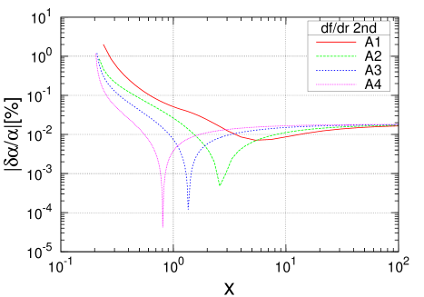
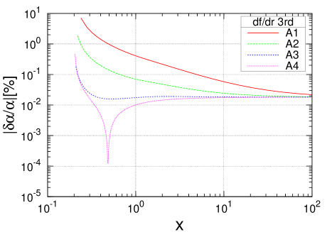
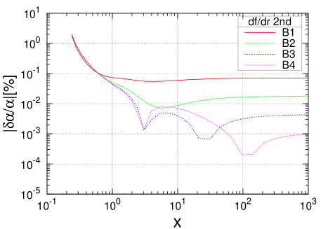
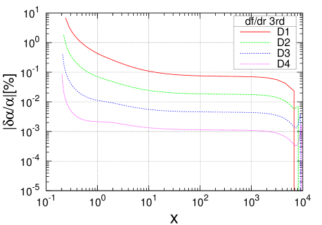
Figure 3: Plots of fractional errors in the lapse $\delta\alpha/\alpha$ along the positive $x$-axis. Plots show the errors with changing the number of radial grid points $r_{i}$ as A1-A4 (top left panel), zenith grid points $\theta_{i}$ as B1-B4 (top right panel), radial grid points $r_{i}$ as A1-A4 (bottom left panel), and all grid points $(r_{i},\theta_{j},\phi_{k})$ as D1-D4 (bottom right panel). In each panel, solid (red), long dashed (green), dashed (blue), and dotted (magenta) lines are in order from lower to higher resolutions. In the top panels, second order finite difference formula is used for calculating radial derivatives, while the third order formula is used in the bottom panels.

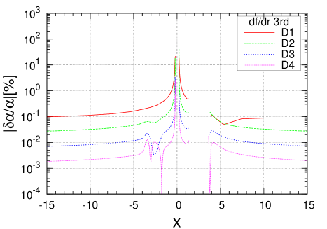
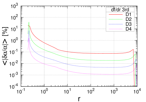
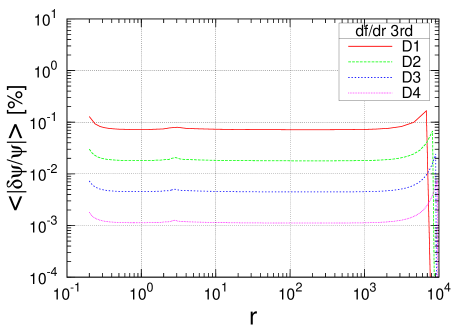
Figure 4: Same as Fig. 3 but for the equal mass BBH data calculated on a single patch Fig. 5. Top panel: Plots for the fractional errors in the lapse $\delta\alpha/\alpha$ for the equal mass BBH data along the positive $x$-axis. Middle panel: averaged fractional errors in the lapse $\left<\left|\delta\alpha/\alpha\right|\right>$. Bottom panel: averaged fractional errors in the conformal factor $\left<\left|\delta\psi/\psi\right|\right>$. Plots show the errors with changing the number of all grid points as D1-D4 in Table 3.

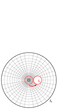
Figure 5: A setup for a single coordinate grid patches for a calculation of equal mass BBH. The radius of coordinate patch doesn’t reflect the actual size.

III.2 Convergence tests

Convergence tests are performed to examine that the code produces solutions with an expected order of finite difference errors, and to find experimentally an (almost) optimally balanced set of resolutions for each coordinate grid $(r_{i},\theta_{j},\phi_{k})$ which is not over resolved in one coordinate direction so as not to waste the computational resources. We find, from convergence tests for a single BH solution, it is necessary to use third order finite difference formula for a radial derivative in the volume source terms in Eq. (7). We also find an optimally balanced resolutions between $r_{i}$ and $\theta_{j}$ grids. From convergence tests for BBH data, we find appropriate resolution for $\phi_{i}$ direction, and number of multipoles. Results for the convergence tests are discussed in this section.

III.2.1 Single BH

For the first test, we compute a single BH solution with mass parameter $M_{1}=2r_{a}=0.4$ (and $M_{2}=0$). Eqs.(25) are solved on a single patch with a single excision region interior of $S_{a}$ for the BH. In Fig. 3, a fractional error of the lapse $\alpha$

$$\left|\frac{\delta\alpha}{\alpha}\right|:=\left|\frac{\alpha-\alpha_{\rm exact}}{\alpha_{\rm exact}}\right|$$ (28)

is plotted along the x-axis for different resolutions in the radial coordinate grids $r_{i}$ (top and bottom left panels), in the zenith angle grids $\theta_{j}$ (top right panel), and in all grids (bottom right panel). These resolutions are tabulated in Table 3, and are indicated by A1-A4, B1-B4, and D1-D4, respectively. In the set A1-A4, the radial resolution $\Delta r$ is doubled, in B1-B4, the zenith angle resolution $\Delta\theta$ is doubled, and in D1-D4, the resolutions in all directions are doubled at each level. Another difference in these results is the order of the finite difference formula used to compute a radial derivative in the volume source term in Eq. (7), where the second order (mid-point) formula is used in the top left and right panels, and third order (Lagrange) formula is used in the bottom left and right panels. It is noticed from the top left panel in Fig.3 that the error does not decrease as ${O}(\Delta r^{2})$ when the number of radial grid points is increased as the parameter sets A1-A4 in Table 3 even for such a spherically symmetric solution.

It appears that there are two reasons for that. In the top right panel, a convergence test is performed changing the number of grid points in zenith angle $\theta_{j}$ as the parameter sets B1-B4. It shows an improvement of the accuracy in ${O}(\Delta\theta^{2})$ in the larger radius $r\gtrsim 100$, that is the error in this region is dominated by the finite differencing in $\theta$ direction. However, the accuracy near the BH is not improved in both tests. In the bottom left panel of Fig. 3, the same convergence test as the top left panel is performed, but the finite difference formula for the radial derivatives is replaced by that of third order Lagrange formula ${O}(\Delta r^{3})$. It shows that it is necessary to set the order of finite difference formula for the radial derivative as ${O}(\Delta r^{3})$ to see ${O}(\Delta r^{2})$ accuracy near the BH. This ${O}(\Delta r^{2})$ error must be due to the mid-point rule used in the numerical integration. While, the error in the larger radius does not decrease in the outer region with the radius $r\gtrsim 100$. Finally, as shown in the bottom right panel of Fig.3 the error decreases in the second order for the set D1-D4, in which the third order finite difference formula is used for the radial derivatives. Convergence test are done also for increasing grid points in $\phi$ directions $\phi_{k}$ and also for changing the number of Legendre expansion as $L=4-10$, but they didn’t change the results for such spherically symmetric BH test.

III.2.2 Equal mass BBH computed with a single patch

In Fig.4, results of convergence tests for equal mass BBH data are plotted. In this test, we used only a single patch shown in Fig.5, where the potential at the radius $r=r_{e}$ rotated by $\pi$ in $\phi$ coordinate is mapped to the excision sphere $S_{e}$ on the same patch to compute the equal mass data when the elliptic equations are solved. This amounts to impose the $\pi$-rotation symmetry about the center of mass which is located at $(r,\theta,\phi)=(d_{s}/2,\pi/2,0)$. In this test, the number of grid points is chosen as D1-D4 in Table 3, separation between the coordinate centers of two BH (a distance between the centers of $S_{a}$ to $S_{e}$) is set as $d_{s}=2.5$, the excision radius of the BH $r_{a}=0.2$, the excision radius of the binary companion $r_{e}=1.125$, and the mass parameters $M_{1}=M_{2}=2r_{a}$. Hereafter, the third order finite difference formula is always used for computing the radial derivatives as discussed in Sec. III.2.1.

In the top panel of Fig. 4, fractional errors of the lapse $|\delta\alpha/\alpha|$ defined in Eq. (28) are plotted along the x-axis near the BH. Because of the excision of the interior of the sphere $S_{e}$ and of the use of Legendre expansion in the elliptic solver, a certain modulation is seen in the errors. Therefore, hereafter we show fractional errors averaged over the number of $(\theta_{j},\phi_{k})$ grids points at a radius $r=r_{i}$ defined by

$$\left<\left|\frac{\delta\alpha}{\alpha}\right|\right>:=\frac{1}{\#({\cal G}_{i})}\sum_{\theta_{j},\phi_{k}\in{\cal G}_{i}}\left|\frac{\alpha-\alpha_{\rm exact}}{\alpha_{\rm exact}}\right|$$ (29)

where writing a grid point $(r_{i},\theta_{j},\phi_{k})$ by $p$, we define a set ${\cal G}_{i}$ by ${\cal G}_{i}:=\left\{(r_{i},\theta_{j},\phi_{k})\ |\ p\in V\setminus S^{\rm in}_{e}\ \mbox{and}\ r_{i}=\mbox{const}\right\}$ where $S^{\rm in}_{e}$ is an interior domain of $S_{e}$. Then, $\#({\cal G}_{i})$ is the number of points included in ${\cal G}_{i}$.

The averaged fractional errors for the lapse are plotted along the radial coordinate $r$ in the middle panel of Fig. 3. As expected, second order convergence is observed when the grid points are increased as D1-D4. In the figure, it is seen that a couple of grid points at the vicinity of BH boundary $S_{a}$ have (averaged) errors as large as $\sim 1\%$ even for the highest resolution D4. This is due to our choice of the boundary $r_{a}=M/2$ as same as the single BH test in the previous section. With this choice, the value of $\alpha$ becomes negative at the BH excision radius $r=r_{a}$. Hence, the fractional error diverges at radii r (depending on $\theta$, and $\phi$) where $\alpha$ crosses zero, even though the grid points are slightly off from the zeros. In this way, the worst possible error in computation for the metric potentials of BH is estimated. Even near the radius for $\alpha=0$, the second order convergence is maintained as seen in the figure. We also show in the bottom panel of Fig. 3, averaged fractional errors for the conformal factor $\psi$. The value of $\psi$ is about 2 near $r=r_{a}$, and for such a potential the convergence of the solution is almost uniform in all radii as observed.

Type	Patch	$r_{a}$	$r_{b}$	$r_{c}$	$r_{e}$	${N_{r}^{\rm f}}$	${N_{r}^{\rm m}}$	$N_{r}$	$N_{\theta}$	$N_{\phi}$	$L$
E1	COCP-1	0.2	$10^{4}$	1.25	1.125	16	20	64	24	24	12
	COCP-2	0.4	$10^{4}$	1.25	1.125	16	20	64	24	24	12
E2	COCP-1	0.2	$10^{4}$	1.25	1.125	32	40	128	48	48	12
	COCP-2	0.4	$10^{4}$	1.25	1.125	32	40	128	48	48	12
E3	COCP-1	0.2	$10^{4}$	1.25	1.125	64	80	256	96	96	12
	COCP-2	0.4	$10^{4}$	1.25	1.125	64	80	256	96	96	12
E4	COCP-1	0.2	$10^{4}$	1.25	1.125	128	160	512	192	192	12
	COCP-2	0.4	$10^{4}$	1.25	1.125	128	160	512	192	192	12
F1	COCP-1	0.2	$10^{2}$	1.25	1.125	16	20	48	24	24	12
	COCP-2	0.4	$10^{2}$	1.25	1.125	16	20	48	24	24	12
	ARCP	5.0	$10^{6}$	6.25	—	4	5	48	24	24	12
F2	COCP-1	0.2	$10^{2}$	1.25	1.125	32	40	96	48	48	12
	COCP-2	0.4	$10^{2}$	1.25	1.125	32	40	96	48	48	12
	ARCP	5.0	$10^{6}$	6.25	—	8	10	96	48	48	12
F3	COCP-1	0.2	$10^{2}$	1.25	1.125	64	80	192	96	96	12
	COCP-2	0.4	$10^{2}$	1.25	1.125	64	80	192	96	96	12
	ARCP	5.0	$10^{6}$	6.25	—	16	20	192	96	96	12
F4	COCP-1	0.2	$10^{2}$	1.25	1.125	128	160	384	192	192	12
	COCP-2	0.4	$10^{2}$	1.25	1.125	128	160	384	192	192	12
	ARCP	5.0	$10^{6}$	6.25	—	32	40	384	192	192	12

Table 4: Grid parameters used in convergence tests for non-equal mass BBH data solved on multiple coordinate patches. The separation of two BHs is set as $d_{s}=2.5$.

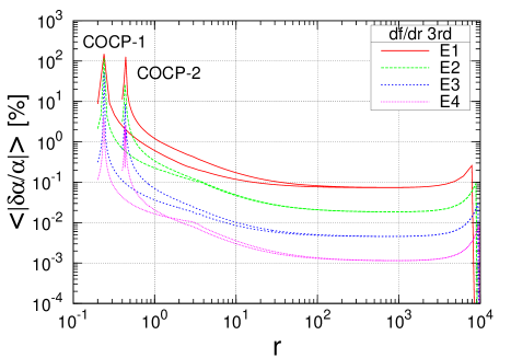
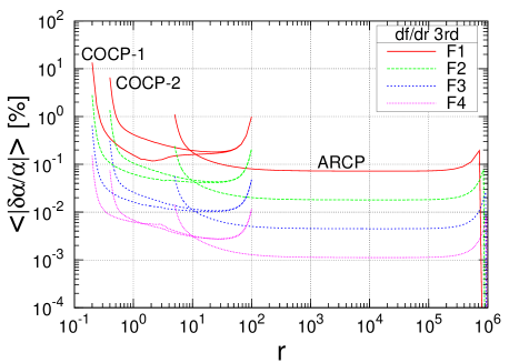
Figure 6: Same as Fig. 3 but averaged fractional errors in the lapse $\left<\left|\delta\alpha/\alpha\right|\right>$ are plotted along the radial coordinate $r$ for the non-equal mass BBH data calculated on multiple patches Fig. 1. Top panel: data computed on two multiple patches with changing the number of grid points as E1-E4 in Table 3. Bottom panel: data computed on three multiple patches with changing the number of all grid points as F1-F4 in Table 3.

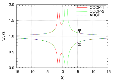
Figure 7: Plots for the conformal factor $\psi$ and the lapse $\alpha$, computed on the three multi patches. The model is the same as that of the bottom panel of Fig. 6.

III.2.3 Non equal mass BBH computed with multiple patches

Convergence test for non-equal mass BBH data using multi coordinate patches discussed in Sec.II is performed with grid parameters presented in Table 4. In the first example, BBH data is computed on two COCP whose boundary radius $r=r_{b}$ is taken large enough to reach to asymptotics $r_{b}=10^{4}$. In this computation, the number of grid points is chosen as E1-E4 in Table 4, in which the resolution in radial grids $r_{i}$ in the region $r>r_{c}$ is increased by 44/24 times of the corresponding level of resolution for equal mass BBH case, D1-D4. Separation between the coordinate centers of two BH is set as $d_{s}=2.5$, the excision radius and mass parameter of the first BH are $r_{a}=0.2$ with $M_{1}=2r_{a}=0.4$, and those of second BH $r_{a}=0.4$ with $M_{2}=2r_{a}=0.8$. The results of the averaged fractional error in the top panel of Fig. 6 is similar to those of the equal mass BBH case in Fig. 4, which proves our multiple patch methods works accurately as expected.

Finally, the BBH data is computed using three multiple patches shown in Fig. 1. The number of grid points is chosen as F1-F4 in Table 4, and the separation is set as $d_{s}=2.5$. In the bottom panel of Fig. 6, the results for the averaged fractional errors $\left<\left|\delta\alpha/\alpha\right|\right>$ are shown. In this computation we decreased the values of mass parameter as $M_{1}=0.8\times 2r_{a}=0.32$ with $r_{a}=0.2$ for the first BH and $M_{2}=0.8\times 2r_{a}=0.64$ with $r_{a}=0.4$ for the second BH, so that the lapse $\alpha$ is always positive even near the BH excision boundary at $r=r_{a}$. As seen in the figure, the error near the BH boundary is decreased about 1/10 of the previous case, although the resolutions near the BH are the same. In the Fig. 7, we present the plots of the potentials $\alpha$ and $\psi$ for the same model to show a smooth transition of potentials from one to the other patch.

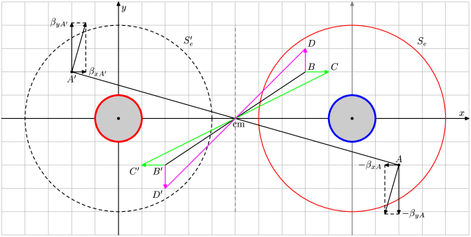
Figure 8: Schematic figure for the $\pi$ rotation symmetry of $x$ and $y$ components of the shift from a region inside to $S^{\prime}_{e}$ to the excised region inside of the sphere $S_{e}$.

Type	$n_{1}$	$n_{0}$	$\Omega$	$\Omega_{\rm s}$	Spin axis	Figures
TU	3.0	1.0	0.3	0.0	—	Fig. 9
TU	2.2	0.005	0.08	0.0	—	Fig. 10
AH	—	0.1	0.08	0.0	—	Figs. 12-18
AH	—	0.005	0.08	0.0	—	Figs. 12-16
AH	—	0.1	0.08	0.1	$z$-axis	Fig. 17
AH	—	0.1	0.08	0.1	$y$-axis	Fig. 18

Table 5: Boundary conditions and their parameters used in the computations for BBH initial data. The first column, Type, denotes the types of boundary conditions used, TU corresponds to Eq. (35), and AH corresponds to apparent horizon boundary conditions Eqs. (36)-(38). The model of Fig.9 is computed with a binary separation $d_{s}=2.8$, a radius of BH excision $r_{a}=0.1$, and a radius of binary excision $r_{e}=1.3$. All the other models are computed with the parameter set D3 in Table 3.

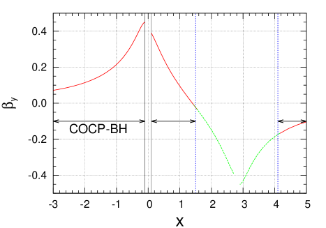
Figure 9: Plots for the $y$-component of shift vector along $x$-axis of BBH initial data computed from the boundary conditions (35). Parameters in the conditions are chosen the same as a solution presented in TU2007 as $n_{1}=3$, $n_{0}=0.1$, and $\Omega=0.3$. Two BH are located at $x=0$ and $x=2.8$. The region inside of the excised sphere $S_{e}$ is interpolated using $\pi$-rotation symmetry. Thin solid (black) vertical lines are the boundaries at $S_{a}$ with the radius $r_{a}=0.1$, and dotted (blue) vertical lines are the boundaries at $S_{e}$ with the radius $r_{e}=1.3$.

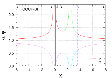
Figure 10: Plots for the conformal factor $\psi$ and lapse function $\alpha$ along the $x$-axis of BBH initial data computed for the boundary condition $(\ref{eq:Initial_bc})$. Parameters in the conditions are chosen as $n_{1}=0.1$, $n_{0}=0.005$ and $\Omega=0.08$. The two BH are located at $x=0$ and $x=2.5$. The region inside of the excised sphere $S_{e}$ is interpolated using $\pi$-rotation symmetry. Thin solid (black) vertical lines are the boundaries at $S_{a}$ with the radius $r_{a}=0.2$, and dotted (blue) vertical lines are the boundaries at $S_{e}$ with the radius $r_{e}=1.125$.

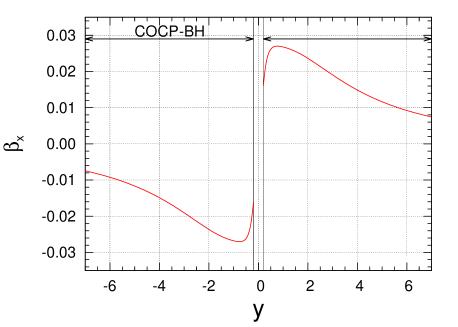
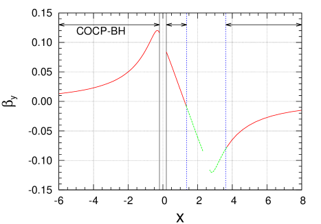
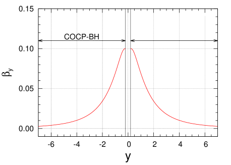
Figure 11: Plots for the same model as Fig. 10 but for the components of the shift $\beta_{i}$. Top panel: $\beta_{x}$ along the $y$-axis. Middle panel: $\beta_{y}$ across the $x$-axis. Bottom panel: $\beta_{y}$ across the $y$-axis.

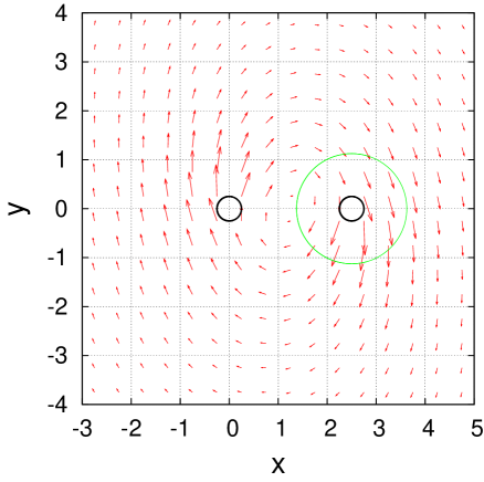
Figure 12: Shift vector on the $xy$-plane of the BBH initial data for the case with AH boundary conditions (36)-(38). Parameters in the conditions are chosen as $n_{0}=0.1$, $\Omega=0.08$, and $\Omega_{\rm s}=0$. The center of mass is located at $x=1.25$ on the $x$-axis. In the computation, the region inside of the left thick circle centered at the origin with a radius $r_{a}=0.2$, and of the thin circle (green) with a radius $r_{e}=1.125$ centered at $x=2.5$ on the $x$-axis are excised. The data inside of the thin circle is interpolated by a symmetry. Note that the center of mass does not coincide with the center of the x-axis.

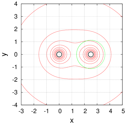
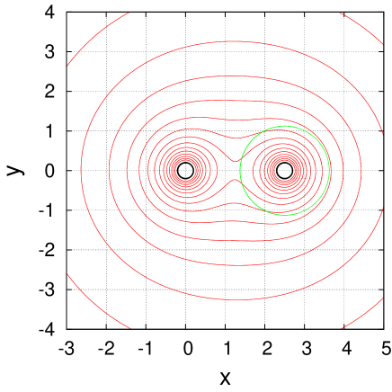
Figure 13: Contour plots on the $xy$-plane for the conformal factor $\psi$ (top panel) and the lapse function $\alpha$ (bottom panel) for the same model as Fig. 12. For $\psi$, we draw isolines from $\psi=1.1$ to $\psi=2.0$ with step $0.1$. For $\alpha$, we draw isolines from $\alpha=0.2$ to $\alpha=0.9$ with step $0.05$.

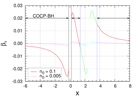
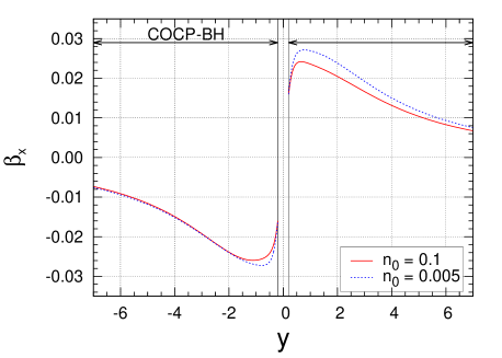
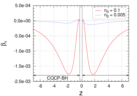
Figure 14: Plots for the $x$-component of the shift $\beta_{x}$ of BBH initial data for the case with AH boundary conditions (36)-(38). Parameters in the conditions are chosen as $n_{0}=0.1$ (solid red lines), and $n_{0}=0.005$ (dashed green lines), with $\Omega=0.08$ and $\Omega_{\rm s}=0$. Top panel: along the $x$-axis. Middle panel: along the $y$-axis. Bottom panel: along the $z$-axis.

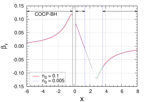
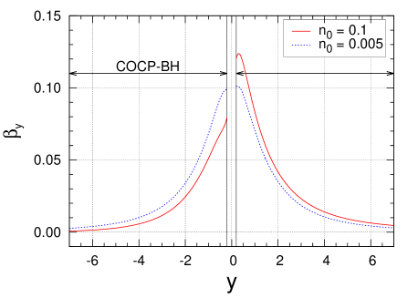
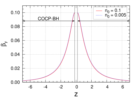
Figure 15: Plots for the same model as Fig. 14 but for the $y$-component of the shift $\beta_{y}$.

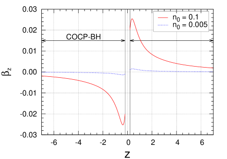
Figure 16: Plots for the same model as Fig. 14 but for the $z$-component of the shift $\beta_{z}$ along the $z$-axis.

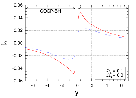
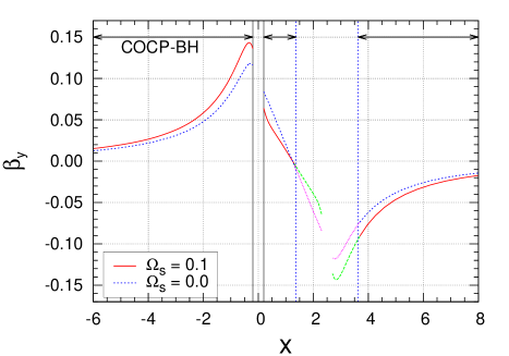
Figure 17: Plots for the components of the shift $\beta_{i}$ of BBH initial data for the case with AH boundary conditions (36)-(38). Parameters in the conditions are chosen as $n_{0}=0.1$ with a spin parameter $\Omega_{\rm s}=0$ (solid red lines), and $\Omega_{\rm s}=0.1$ (dashed green lines). The spins are aligned to the orbital angular momentum (i.e. parallel to $z$-axis). Top panel: $\beta_{x}$ component along the $y$-axis. Bottom panel: $\beta_{y}$ component along the $x$-axis. Solid red curves correspond to those in Figs. 14–16.

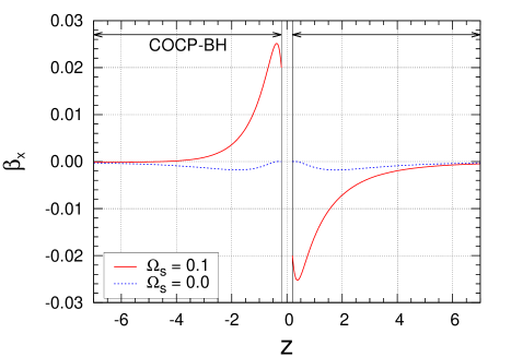
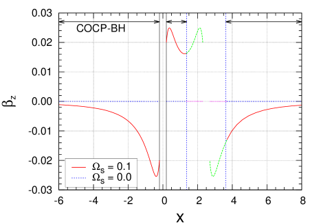
Figure 18: Same as Fig.17, but the direction of the spin is aligned parallel to the $y$-axis. Top panel: $\beta_{x}$ component along the $z$-axis. Middle panel: $\beta_{z}$ component along the $x$-axis. Bottom panel: $\beta_{z}$ component along the $y$-axis.

IV Initial data for binary black holes

Finally we present examples for initial data sets for equal mass BBH, which have been widely used for BBH merger simulations in the literature. Among several formulations for computing such data sets (see e.g. NRreview ; Cook:2000vr and references therein), we adopt Isenberg-Wilson-Mathews (IWM) formulation. In this section, we show the solutions computed from two different types of boundary conditions. The first are simple boundary conditions used in our previous paper TU2007 . The second are the apparent horizon boundary conditions, which have been used to compute quasi-circular initial data for BBH (see e.g. Gourgoulhon:2005ng ; Booth:2005qc ; Cook:2000vr ; BBH_QE ).

IV.1 IWM formulation and boundary conditions

IWM formulation has been widely used for constructing quasi-equilibrium initial data for binary compact objects. We summarize the basic equations below (for more details see e.g. Cook:2000vr ; ISEN78 ; WM89 ). The spacetime metric on $\Sigma_{t}$ is written in 3+1 form as

$$ds^{2} = g_{\mu\nu}dx^{\mu}dx^{\nu}$$ (30)

$$= -\alpha^{2}dt^{2}+\gamma_{ij}(dx^{i}+\beta^{i}dt)(dx^{j}+\beta^{j}dt),$$

where the spatial three metric $\gamma_{ij}$ on the slice $\Sigma_{t}$ is assumed to be conformally flat $\gamma_{ij}=\psi^{4}f_{ij}$. Here, field variables $\psi,\alpha$, and $\beta^{i}$ are the conformal factor, lapse, and shift vector, respectively. We also assume maximal slicing to $\Sigma_{t}$, so that the trace of the extrinsic curvature $K_{ij}:=-\frac{1}{2\alpha}(\mbox{\pounds}_{t}\gamma_{ij}-\mbox{\pounds}_{\beta}\gamma_{ij})$ vanishes. Then, writing its tracefree part $A_{ij}$, the conformally rescaled quantity $\tilde{A}_{ij}$ becomes

$${\tilde{A}}_{ij}=\frac{1}{2\alpha}\left(\partial_{i}{\tilde{\beta}}_{j}+\partial_{j}{\tilde{\beta}}_{i}-\frac{2}{3}f_{ij}\partial_{k}{\tilde{\beta}}^{k}\right)\ ,$$ (31)

where the derivative $\partial_{i}$ is associated with the flat metric $f_{ij}$, and conformally rescaled quantities with tilde are defined by $\tilde{A}_{i}{}^{j}=A_{i}{}^{j}$ and ${\tilde{\beta}}^{i}=\beta^{i}$, whose indexes are lowered (raised) by $f_{ij}$ ($f^{ij}$). The system to be solved, which are Hamiltonian and momentum constraints and the spatial trace of the Einstein’s equation, becomes

$$\Delta\psi = -\frac{\psi^{5}}{8}{\tilde{A}}_{ij}{\tilde{A}}^{ij},$$ (32)

$$\Delta\beta_{i} = -2\,\alpha\,{\tilde{A}}_{i}{}^{j}\partial_{j}\ln\frac{\psi^{6}}{\alpha}-\frac{1}{3}\partial_{i}\partial_{j}{\tilde{\beta}}^{j},$$ (33)

$$\Delta(\alpha\psi) = \frac{7}{8}\,\alpha\,\psi^{5}{\tilde{A}}_{ij}{\tilde{A}}^{ij},$$ (34)

where $\Delta:=\partial_{i}\partial^{i}$ is a flat Laplacian. It is noted that, for the shift equation (33), the Cartesian components are solved on the spherical coordinates.

As a first set of the boundary conditions at the BH excision boundary $S_{a}$ and at the boundary of computational domain $S_{b}$ for the above system Eqs. (32)-(34), we choose the following for simplicity,

$$\begin{aligned} \left.\psi\right|_{r=r_{a}}&=n_{1}\\ \left.\beta^{i}\right|_{r=r_{a}}&=-\,\Omega\,\phi_{\rm cm}^{i}\\ \left.\alpha\right|_{r=r_{a}}&=n_{0}\end{aligned}\qquad\mbox{and}\qquad\begin{aligned} \left.\psi\right|_{r=r_{b}}&=1.0\\ \left.\beta^{i}\right|_{r=r_{b}}&=0.0\\ \left.\alpha\right|_{r=r_{b}}&=1.0\end{aligned}$$ (35)

where $n_{1}$ and $n_{0}$ are arbitrary positive constants taken as $n_{1}\gtrsim 2$ and $n_{0}\lesssim 1$, $\phi_{\rm cm}^{i}=(-y_{\rm cm},x_{\rm cm},0)$ is the rotational vector with respect to the center of mass of the binary associated with coordinates $(x_{\rm cm},y_{\rm cm},z_{\rm cm}):=(x-d,y,z)$, and $\Omega$ corresponds to the orbital angular velocity. The radius $r_{b}$ is taken large enough as in the test problems in Sec. III. Despite the fact that the boundary conditions above may be of the simplest type for IWM formulation deduced for acquiring BBH data with non-zero orbital angular momentum in an asymptotically flat system, they capture the qualitative functional behavior of the unknown fields $\{\psi,\alpha,\beta^{i}\}$, as more realistic boundary conditions mentioned below. The solutions calculated from these boundary conditions (35) are compared with our previous code TU2007 that uses a different structure for the multiple spherical coordinate patches, as well as those solutions of different boundary conditions.

For a second set of the boundary conditions, we impose more realistic boundary conditions at the BH boundary $S_{a}$, in particular those that represent apparent horizons in equilibrium Gourgoulhon:2005ng ; Booth:2005qc ; Cook:2000vr ; BBH_QE ,

$$\left.\frac{\partial\psi}{\partial r}+\frac{\psi}{2r}\right|_{r=r_{a}} = -\frac{\psi^{3}}{4}K_{ij}s^{i}s^{j},$$ (36)

$$\left.\beta^{i}\right|_{r=r_{a}} = \frac{n_{0}}{\psi^{2}}s^{i}-\Omega\,\phi^{i}_{\rm cm}-\Omega_{\rm s}\,\phi_{\rm s}^{i},$$ (37)

$$\left.\alpha\right|_{r=r_{a}} = n_{0},$$ (38)

where $n_{0}$ is an arbitrary positive constant for which we choose $n_{0}\lesssim 0.1$, $s^{i}$ is the unit normal to the sphere $S_{a}$, and $\Omega_{\rm s}$ represents the spin of each black hole. The vector $\phi_{\rm s}^{i}$ is the rotational vectors with respect to the coordinate center of BH that generates the BH spin. The spin axis is not necessary parallel to the $z$-axis. Demanding the sphere $S_{a}$ to be an apparent horizon (AH) results in Eq. (36), while demanding the horizon to be in equilibrium results in Eq. (37).

For the present calculations for BBH initial data, we also assume $\pi$-rotation symmetry of the system around the center of mass. That is, two BH have equal masses, and $\pi$-rotation symmetric spins if any. In other words, the same boundary conditions are imposed on both BH. In those cases, a single patch method discussed in Sec. III.2.1 can be used for simplicity. As shown in Fig.8, the metric potentials are mapped to the excised sphere $S_{e}$ from the corresponding sphere $S^{\prime}_{e}$, taking into account the parity of the variables with respect to the $\pi$-rotation. As an example, the $\pi$-rotation symmetries of the shift components on the $xy$-plane are shown schematically (the shift at $A^{\prime}$ is mapped to point $A$), together with the corresponding rules for the derivatives of a function along the $x$-axis inside the excised sphere ($B^{\prime}C^{\prime}$ mapped to $BC$) and along the $y$-axis ($B^{\prime}D^{\prime}$ mapped to $BD$). In terms of the center of mass coordinates, the $\pi$-rotation symmetries of the components of the shift vector become

$$\beta_{x}(-x_{\rm cm},-y_{\rm cm},z_{\rm cm}) = -\beta_{x}(x_{\rm cm},y_{\rm cm},z_{\rm cm})\ ,$$

$$\beta_{y}(-x_{\rm cm},-y_{\rm cm},z_{\rm cm}) = -\beta_{y}(x_{\rm cm},y_{\rm cm},z_{\rm cm}).$$

The $z$-component $\beta_{z}$ is mapped as a scalar quantity.

Mapped quantities are used in the elliptic equation solver when the sources of surface integrals on the excised sphere $S_{e}$, Eq. (7) are evaluated. Also, at the end of each iteration step, obtained potentials $\{\psi,\alpha,\beta_{i}\}$ between the spheres $S_{a}$ and $S^{\prime}_{e}$ are interpolated inside the sphere $S_{e}$ following the same rules for the parity of each variable. At the end we have the solution at every point inside $S_{b}$ and outside of the two black holes of radius $r_{a}$ positioned at the origin and at $x=d_{s}$ on the $x$-axis.

In the case of no spins $\Omega_{\rm s}=0$, or spins are parallel to one of coordinate axis, additional symmetries with respect to the $xy|_{\rm cm}$ plane occur. In our previous codes UryuCF ; UryuWL ; TU2007 , a part or all of these symmetries were encoded in the elliptic solver, for a computational domain was reduced by assuming the symmetries so that only a part of the whole hypersurface $\Sigma_{t}$ was solved. In cocal, we are solving in the whole $\Sigma_{t}$ and therefore such symmetries are satisfied in the solution within negligible numerical errors.

IV.2 Solutions for BBH initial data

Finally, we present the BBH initial data sets computed from the above formulation with several parameter sets for boundary conditions listed in Table 5. As we concentrate on testing the cocal code, we do not discuss much of the physical contents of the initial data sets, but display the plots of the fields to check their behaviors.

In Fig. 9, we calculated BBH data for the same model as shown in our previous paper TU2007 for a comparison. Parameters in the boundary condition (35) are chosen as $n_{1}=3.0$, $n_{0}=1.0$, and $\Omega=0.3$. Only in this model, we choose the binary separation as $d_{s}=2.8$ and the BH excision radius $r_{a}=0.1$. We find the solution agrees well with Fig. 11 of TU2007 as expected, although the structures of coordinate patches are different in each code. In Figs. 10, and 11, We use the same boundary conditions (35) but with different parameters which may be more common values for the BBH data. In the computation, the grid parameters used are D3 in Table 3. When the value of $\Omega$ is increased, the magnitude of the lapse and the conformal factor remain almost the same, while the magnitude of the components of the shift increase with the functional behavior staying the same. For example when $\Omega=0.1$, $\beta_{x}$ on the $y$-axis varies between $\pm 0.05$ while $\beta_{y}$ on the $x$-axis varies between $\pm 0.15$. For this boundary conditions, the code blows up when $\Omega$ is approximately greater than $0.2$.

Solutions for the BBH initial data with the AH boundary conditions (36)-(38) are shown in Figs. 12–16. In this calculation, the resolution is D3 in Table 3 with $\Omega=0.08$ and $\Omega_{\rm s}=0$. The shift vector plots and the contour plots of the conformal factor $\psi$ and the lapse $\alpha$ in $xy$-plane are for the model with $n_{0}=0.1$. The behavior of the field $\psi$ and $\alpha$ are analogous to those from the simple boundary condition (35) shown in Fig. 10. Because of the choice $\Omega_{\rm s}=0$, the solution satisfies xy-plane symmetry.

From a comparison between the results of parameters $n_{0}=0.1$ and $0.005$ shown in Figs. 14-16, it is found that the results with $n_{0}=0.005$ becomes more similar to the results of the first boundary conditions (35) shown in Fig.11. For example, it is most evident in the plot for $\beta_{y}$ along the $y$-axis, Fig.15 middle panel and Fig.11 bottom panel. This seems to be a correct behavior because the first term of Eq. (37) contributes less as the value of alpha (parameter $n_{0}$) become smaller . However, it is not expected that there is a solution in the limit of $n_{0}\rightarrow 0$, in fact, for both types of boundary conditions iterations diverge when the $n_{0}\lesssim 0.004$ in the cocal code.

All of the solutions above have zero black hole spins. Setting spins $\Omega_{\rm s}=0.1$ in the same direction as the orbital motion (rotation on the xy-plane) we get a solution similar to Figs. 14-16 except for $\beta_{x}$ along the y-axis and $\beta_{y}$ along the x-axis. The results with and without spins are compared in Fig. 17 for the case with $n_{0}=0.1$. For more general black hole spins we obtain Fig.18 where we have taken a spin $\Omega_{\rm s}=0.1$ along the y-axis. In these plots for the solutions with the spins, we confirm that all components of the shift vectors behave correctly along each coordinate axis.

V Discussion

Although the numerical method presented in this paper may seem similar to the one presented in our previous paper TU2007 , the robustness of the convergence and the control of the numerical errors are largely improved. In some cases, the previous method failed to compute a continuous solution at the interface between multiple patches during the iterations, and therefore a convergence to a solution couldn’t be achieved. A major reason for this failure turned out to be a lack of enough overlap region between coordinate patches. The numerical errors of the field variables are relatively larger near the boundary of computational domain as seen, for example, in Fig.6. Hence if the overlap region is small, those potentials with larger numerical errors overlap, which seems to cause the non-convergence of the iteration. In the cocal code, the overlap region is almost as large as the whole domain for the two coordinate patch configuration, and is large enough even for the three coordinate patch configuration. We have never observed so far a discontinuous behavior of a field in the solutions of cocal.

The cocal code currently runs only on a serial processor, which is sufficient to maintain the accuracy presented in Sec.III. In the computation for BBH initial data shown in Sec.IV, the size of main memory and CPU times per 1 iteration cycle used by cocal are about 800MB 50sec for D3 grid, and 6GB 8min for D4 grid, and around 50-150 iterations are needed for a convergence, where the iterations start from an initial guess $\psi=\alpha=1$ and $\beta_{i}=0$. Because we use second order accurate formulas in cocal, we can decrease the numerical error by two orders of magnitude with $10$ times more grid points in each direction, that is, $10^{3}$ more grids in total. Considering specs of common parallel computer systems it seems to be feasible to achieve this accuracy by parallelizing cocal. We have started to develop a prototype of such parallelized cocal code, whose results would be presented elsewhere.

The most advantageous feature of cocal would be its simplicity in coding. This helps the users to introduce more complex physics on top of the current code. For example, we have developed subroutines for solving spatially conformally flat data (IWM formulation) first, and later added subroutines for solving non-conformally flat data (waveless formulation) on top. In the same way, it will be straight forward to incorporate subroutines to solve electromagnetic fields, which enables us to investigate for example magnetar models. We proceed to develop codes for computing various kinds of astrophysically realistic equilibriums and quasi-equilibrium data and provide the results to applications including initial data for numerical relativity simulations. We plan for making the cocal code and computed initial data sets available for public in the near future.

Appendix A Computations for homogeneous solutions

In this Appendix, we show a concrete derivation for the homogeneous solution $\chi(x)$ used in the elliptic solver (6) for two cases, one with Neumann boundary condition at the inner boundary sphere $S_{a}$ and Dirichlet boundary condition at the outer boundary sphere $S_{b}$, and the other with Dirichlet conditions at both $S_{a}$ and $S_{b}$. We summarize the other cases in the next Appendix B.

As explained in Sec. II.3, the solution of $\mathcal{L}\Phi=S$ is written $\Phi(x)=\chi(x)+\Phi_{\rm INT}(x)$ to impose certain boundary conditions at the two spheres $S_{a}$ and $S_{b}$. In order to do so, the homogeneous solution $\chi$ of the Laplacian is split into two functions $\chi_{a}(x)$ and $\chi_{b}(x)$ as $\chi(x)=\chi_{a}(x)+\chi_{b}(x)$. Both are solutions of Laplace equations, and one for the exterior of the sphere $S_{a}$ and the other for the interior of the sphere $S_{b}$ (see Fig. 19). Since $r^{\ell},\ r^{-\ell-1}$ are the solutions of the radial part of the Laplacian, the contribution $\chi_{a}$ is taken to be a series of $r^{-\ell-1}$, while the contribution $\chi_{b}$ to be a series of $r^{\ell}$. Therefore, we write

$$\chi_{a}(x) = \frac{1}{4\pi}\sum_{\ell=0}^{\infty}\sum_{m=0}^{\ell}\epsilon_{m}\frac{(\ell-m)!}{(\ell+m)!}P_{\ell}^{m}(\cos\theta)r^{-\ell-1}\times\qquad$$ (39)

$$\times[A_{\ell m}\cos(m\phi)+B_{\ell m}\sin(m\phi)]\qquad$$

$$\chi_{b}(x) = \frac{1}{4\pi}\sum_{\ell=0}^{\infty}\sum_{m=0}^{\ell}\epsilon_{m}\frac{(\ell-m)!}{(\ell+m)!}P_{\ell}^{m}(\cos\theta)r^{\ell}\times\qquad$$ (40)

$$\times[C_{\ell m}\cos(m\phi)+D_{\ell m}\sin(m\phi)]\qquad$$

where $A_{\ell m}$, $B_{\ell m}$, $C_{\ell m}$, and $D_{\ell m}$ are constants. One common choice is

$$\left.\frac{\partial\Phi}{\partial r}\right|_{r=r_{a}} = \left.\frac{\partial\Phi_{\rm BC}}{\partial r}\right|_{r=r_{a}}$$ (41)

$$\left.\Phi\right|_{r=r_{b}} = \left.\Phi_{\rm BC}\right|_{r=r_{b}},$$ (42)

where $\frac{\partial\Phi_{\rm BC}}{\partial r}|_{r=r_{a}}$ and $\Phi_{\rm BC}|_{r=r_{b}}$ are known functions defined at boundaries $S_{a}$ and $S_{b}$, respectively; we consider the case with Neumann boundary condition at the inner surface $S_{a}$ and Dirichlet at the outer one $S_{b}$.

From boundary condition Eq. (41) with the use of Eqs. (39), (40), (6), (7), and the orthogonality relations

$$\int_{0}^{\pi}P_{\ell}^{m}(\cos\theta)P_{\ell^{\prime}}^{m}(\cos\theta)\sin\theta d\theta=\frac{2}{2\ell+1}\frac{(\ell+m)!}{(\ell-m)!}\delta_{\ell\ell^{\prime}}$$

$$\int_{0}^{2\pi}\sin(m\phi)\cos(m^{\prime}\phi)d\phi=0\qquad\qquad\qquad\qquad$$

$$\int_{0}^{2\pi}\cos(m\phi)\cos(m^{\prime}\phi)d\phi=\frac{2\pi}{\epsilon_{m}}\delta_{mm^{\prime}}\qquad\qquad\quad$$

we get

$$-\frac{\ell+1}{r_{a}^{\ell+2}}A_{\ell m}+\ell r_{a}^{\ell-1}C_{\ell m}=(2\ell+1)\times\qquad\qquad$$

$$\int_{0}^{\pi}\int_{0}^{2\pi}\left(\frac{\partial\Phi_{\rm BC}}{\partial r}-\frac{\partial\Phi_{\rm INT}}{\partial r}\right)_{r=r_{a}}P_{\ell}^{m}(\cos\theta)\cos(m\phi)d\Omega$$

(43)

$$-\frac{\ell+1}{r_{a}^{\ell+2}}B_{\ell m}+\ell r_{a}^{\ell-1}D_{\ell m}=\frac{2(2\ell+1)}{\epsilon_{m}}\times\qquad\qquad$$

$$\int_{0}^{\pi}\int_{0}^{2\pi}\left(\frac{\partial\Phi_{\rm BC}}{\partial r}-\frac{\partial\Phi_{\rm INT}}{\partial r}\right)_{r=r_{a}}P_{\ell}^{m}(\cos\theta)\sin(m\phi)d\Omega$$

Using now boundary condition Eq. (42) and again the same equations we get

$$r_{b}^{-\ell-1}A_{\ell m}+r_{b}^{\ell}C_{\ell m}=(2\ell+1)\times\qquad\qquad$$

$$\int_{0}^{\pi}\int_{0}^{2\pi}\left(\Phi_{\rm BC}-\Phi_{\rm INT}\right)_{r=r_{b}}P_{\ell}^{m}(\cos\theta)\cos(m\phi)d\Omega\qquad$$ (45)

$$r_{b}^{-\ell-1}B_{\ell m}+r_{b}^{\ell}D_{\ell m}=\frac{2(2\ell+1)}{\epsilon_{m}}\times\qquad\qquad$$

$$\int_{0}^{\pi}\int_{0}^{2\pi}\left(\Phi_{\rm BC}-\Phi_{\rm INT}\right)_{r=r_{b}}P_{\ell}^{m}(\cos\theta)\sin(m\phi)d\Omega\qquad$$ (46)

The system of four equations with respect to $A_{\ell m}$, $B_{\ell m}$, $C_{\ell m}$, $D_{\ell m}$ can be solved to yield

$$A_{\ell m}\left[1+\frac{\ell}{\ell+1}\left(\frac{r_{a}}{r_{b}}\right)^{2\ell+1}\right] = \frac{\ell(2\ell+1)}{\ell+1}r_{a}^{\ell+1}\left(\frac{r_{a}}{r_{b}}\right)^{\ell}\int_{S_{b}}(\Phi_{\rm BC}-\Phi_{\rm INT})P_{\ell}^{m}(\cos\theta)\cos(m\phi)d\Omega$$

$$-\frac{2\ell+1}{\ell+1}r_{a}^{\ell+2}\int_{S_{a}}\left(\frac{\partial\Phi_{\rm BC}}{\partial r}-\frac{\partial\Phi_{\rm INT}}{\partial r}\right)P_{\ell}^{m}(\cos\theta)\cos(m\phi)d\Omega,$$

$$C_{\ell m}\left[1+\frac{\ell}{\ell+1}\left(\frac{r_{a}}{r_{b}}\right)^{2\ell+1}\right] = (2\ell+1)b^{-\ell}\int_{S_{b}}(\Phi_{\rm BC}-\Phi_{\rm INT})P_{\ell}^{m}(\cos\theta)\cos(m\phi)d\Omega$$

$$+\frac{2\ell+1}{\ell+1}\frac{r_{a}^{2}}{r_{b}^{\ell+1}}\left(\frac{r_{a}}{r_{b}}\right)^{\ell}\int_{S_{a}}\left(\frac{\partial\Phi_{\rm BC}}{\partial r}-\frac{\partial\Phi_{\rm INT}}{\partial r}\right)P_{\ell}^{m}(\cos\theta)\cos(m\phi)d\Omega,$$

$$B_{\ell m}\left[1+\frac{\ell}{\ell+1}\left(\frac{r_{a}}{r_{b}}\right)^{2\ell+1}\right] = \frac{2\ell(2\ell+1)}{(\ell+1)\epsilon_{m}}r_{a}^{\ell+1}\left(\frac{r_{a}}{r_{b}}\right)^{\ell}\int_{S_{b}}(\Phi_{\rm BC}-\Phi_{\rm INT})P_{\ell}^{m}(\cos\theta)\sin(m\phi)d\Omega$$

$$-\frac{2(2\ell+1)}{(\ell+1)\epsilon_{m}}r_{a}^{\ell+2}\int_{S_{a}}\left(\frac{\partial\Phi_{\rm BC}}{\partial r}-\frac{\partial\Phi_{\rm INT}}{\partial r}\right)P_{\ell}^{m}(\cos\theta)\sin(m\phi)d\Omega,$$

$$D_{\ell m}\left[1+\frac{\ell}{\ell+1}\left(\frac{r_{a}}{r_{b}}\right)^{2\ell+1}\right] = \frac{2(2\ell+1)}{\epsilon_{m}}r_{b}^{-\ell}\int_{S_{b}}(\Phi_{\rm BC}-\Phi_{\rm INT})P_{\ell}^{m}(\cos\theta)\sin(m\phi)d\Omega$$

$$+\frac{2(2\ell+1)}{(\ell+1)\epsilon_{m}}\frac{r_{a}^{2}}{r_{b}^{\ell+1}}\left(\frac{r_{a}}{r_{b}}\right)^{\ell}\int_{S_{a}}\left(\frac{\partial\Phi_{\rm BC}}{\partial r}-\frac{\partial\Phi_{\rm INT}}{\partial r}\right)P_{\ell}^{m}(\cos\theta)\sin(m\phi)d\Omega.$$

Substituting the above in Eqs. (39) and (40), we have

$$\chi_{a}(x)+\chi_{b}(x) = \frac{1}{4\pi}\sum_{\ell=0}^{\infty}\sum_{m=0}^{\ell}\epsilon_{m}\frac{(\ell-m)!}{(\ell+m)!}P_{\ell}^{m}(\cos\theta)\times$$ (47)

$$\left\{(2\ell+1)\left(\frac{r_{a}}{r_{b}}\right)^{\ell}\frac{\left(\frac{r}{r_{a}}\right)^{\ell}+\frac{\ell}{\ell+1}\left(\frac{r_{a}}{r}\right)^{\ell+1}}{1+\frac{\ell}{\ell+1}\left(\frac{r_{a}}{r_{b}}\right)^{2\ell+1}}\int_{S_{b}}[\Phi_{\rm BC}-\Phi_{\rm INT}]P_{\ell}^{m}(\cos\theta^{\prime})\cos[m(\phi-\phi^{\prime})]d\Omega^{\prime}\right.$$

$$\left.+\frac{-2\ell-1}{\ell+1}\frac{r_{a}^{\ell+2}}{r_{b}^{\ell+1}}\frac{\left(\frac{r_{b}}{r}\right)^{\ell+1}-\left(\frac{r}{r_{b}}\right)^{\ell}}{1+\frac{\ell}{\ell+1}\left(\frac{r_{a}}{r_{b}}\right)^{2\ell+1}}\int_{S_{a}}\left(\frac{\partial\Phi_{\rm BC}}{\partial r}-\frac{\partial\Phi_{\rm INT}}{\partial r}\right)P_{\ell}^{m}(\cos\theta^{\prime})\cos[m(\phi-\phi^{\prime})]d\Omega^{\prime}\right\}.$$

Similarly, when we have Dirichlet boundary conditions on both the inner and the outer spheres $S_{a}$ and $S_{b}$,

$$\left.\Phi\right|_{r=r_{a}} = \left.\Phi_{\rm BC}\right|_{r=r_{a}},$$ (48)

$$\left.\Phi\right|_{r=r_{b}} = \left.\Phi_{\rm BC}\right|_{r=r_{b}},$$ (49)

the contribution to the potential will be

$$\chi_{a}(x)+\chi_{b}(x) = \frac{1}{4\pi}\sum_{\ell=0}^{\infty}\sum_{m=0}^{\ell}\epsilon_{m}\frac{(\ell-m)!}{(\ell+m)!}P_{\ell}^{m}(\cos\theta)\times$$ (50)

$$\left\{(2\ell+1)\left(\frac{r_{a}}{r_{b}}\right)^{\ell}\frac{\left(\frac{r}{r_{a}}\right)^{\ell}-\left(\frac{r_{a}}{r}\right)^{\ell+1}}{1-\left(\frac{r_{a}}{r_{b}}\right)^{2\ell+1}}\int_{S_{b}}[\Phi_{\rm BC}-\Phi_{\rm INT}]P_{\ell}^{m}(\cos\theta^{\prime})\cos[m(\phi-\phi^{\prime})]d\Omega^{\prime}\right.$$

$$\left.+(2\ell+1)\left(\frac{r_{a}}{r_{b}}\right)^{\ell+1}\frac{\left(\frac{r_{b}}{r}\right)^{\ell+1}-\left(\frac{r}{r_{b}}\right)^{\ell}}{1-\left(\frac{r_{a}}{r_{b}}\right)^{2\ell+1}}\int_{S_{a}}[\Phi_{\rm BC}-\Phi_{\rm INT}]P_{\ell}^{m}(\cos\theta^{\prime})\cos[m(\phi-\phi^{\prime})]d\Omega^{\prime}\right\}$$

The final solution will be obtained from the iteration of

$$\Phi(x)\ =\ \chi(x)\ +\ \Phi_{\rm INT}(x)\ =\ \chi_{a}(x)\ +\ \chi_{b}(x)\ +\ \Phi_{\rm INT}(x)$$

where $\chi_{a}+\chi_{b}$ are taken from Eq. (47) or (50) depending on the boundary condition. For the other boundary value problem, $\chi(x)=\chi_{a}(x)+\chi_{b}(x)$ is modified accordingly as shown in the next Appendix.

Appendix B Green’s functions and surface integrals

In this Appendix, we present the explicit forms of the kernel functions denoted by $G^{\rm BC}(x,x^{\prime})$ in Eq.(12), which appear in the surface integrals of the homogeneous solution $\chi(x)$ (11). Various types of boundary conditions are imposed on a spherical domain bounded by two concentric spheres $S_{a}$ and $S_{b}$, and the corresponding kernel functions available in cocal are tabulated in Table 1. In TU2007 we used Green’s functions $G^{\rm NB}(x,x^{\prime})$, $G^{\rm DD}(x,x^{\prime})$, and $G^{\rm ND}(x,x^{\prime})$. Here we construct also $G^{\rm DN}(x,x^{\prime})$, $G^{\rm NN}(x,x^{\prime})$, $G^{\rm RD}(x,x^{\prime})$.

The surface integral

$$\chi(x) = \frac{1}{4\pi}\int_{S_{a}\cup S_{b}}\left[G^{\rm BC}(x,x^{\prime})\nabla^{\prime\alpha}\widehat{\Phi}(x^{\prime})\right.$$ (51)

$$\qquad\qquad\left.-\widehat{\Phi}(x^{\prime})\nabla^{\prime\alpha}G^{\rm BC}(x,x^{\prime})\right]dS^{\prime}_{\alpha},$$

where $\widehat{\Phi}(x^{\prime}):=\Phi^{\rm BC}(x^{\prime})-{\Phi_{\rm INT}}(x^{\prime})$, are written below for both the exterior and the interior problem. Noticing that $dS^{\prime}_{\alpha}$ is pointing outward, $S_{a}$ and $S_{b}$ are the concentric spheres, and $\nabla^{\prime\alpha}f(x^{\prime})\,dS^{\prime}_{\alpha}=\partial_{r^{\prime}}f\,r^{\prime 2}d\Omega^{\prime}$, we have

$$\chi_{a}=\frac{1}{4\pi}\int_{S_{a}}\sum_{\ell=0}^{\infty}\left[-g_{\ell}^{\rm BC}(r,r^{\prime})\partial_{r^{\prime}}\widehat{\Phi}\,+\,\partial_{r^{\prime}}g_{\ell}^{\rm BC}(r,r^{\prime})\,\widehat{\Phi}\right]_{r^{\prime}=r_{a}}\!\!\!\!\times$$

$$\sum_{m=0}^{\ell}\epsilon_{m}\frac{(\ell-m)!}{(\ell+m)!}P_{\ell}^{m}(\cos\theta)P_{\ell}^{m}(\cos\theta^{\prime})\cos[m(\phi-\phi^{\prime})]r_{a}^{2}d\Omega^{\prime},$$

(52)

and

$$\chi_{b}=\frac{1}{4\pi}\int_{S_{b}}\sum_{\ell=0}^{\infty}\left[g_{\ell}^{\rm BC}(r,r^{\prime})\partial_{r^{\prime}}\widehat{\Phi}\,-\,\partial_{r^{\prime}}g_{\ell}^{\rm BC}(r,r^{\prime})\,\widehat{\Phi}\right]_{r^{\prime}=r_{b}}\!\!\!\!\times$$

$$\sum_{m=0}^{\ell}\epsilon_{m}\frac{(\ell-m)!}{(\ell+m)!}P_{\ell}^{m}(\cos\theta)P_{\ell}^{m}(\cos\theta^{\prime})\cos[m(\phi-\phi^{\prime})]r_{b}^{2}d\Omega^{\prime}.$$

(53)

Note that these $\chi_{a}$ and $\chi_{b}$ in this section are defined differently from those in the previous section, Eq. (39) and (40). As shown in Fig. 19, we denote by $r_{a}$ the radius of the sphere $S_{a}$ for the exterior problem and by $\chi_{a}$ the corresponding integral and by $r_{b}$ the radius of the sphere $S_{b}$ for the interior problem and $\chi_{b}$ the corresponding integral.

Figure 19: Surface integral for the exterior and the interior of a sphere

B.1 Kernel function $G^{\rm NB}(x,x^{\prime})$

The radial part for the kernel function without boundary $G^{\rm NB}(x,x^{\prime})$, is

$$g^{\rm NB}_{\ell}(r,r^{\prime})=\frac{r_{<}^{\ell}}{r_{>}^{\ell+1}},$$ (54)

where $r_{>}:=\max\{r,r^{\prime}\}$, and $r_{<}:=\min\{r,r^{\prime}\}$. The radial part of the kernel function in the surface integral on $S_{a}$ (52) becomes

$$g_{\ell}^{\rm NB}(r,r_{a})=\frac{r_{a}^{\ell}}{r^{\ell+1}},\ \ \ \ \partial_{r^{\prime}}g_{\ell}^{\rm NB}(r,r_{a})=\ell\frac{r_{a}^{\ell-1}}{r^{\ell+1}},$$ (55)

while the surface integral on $S_{b}$,

$$g_{\ell}^{\rm NB}(r,r_{b})=\frac{r^{\ell}}{r_{b}^{\ell+1}},\ \ \ \ \partial_{r^{\prime}}g_{\ell}^{\rm NB}(r,r_{a})=-(\ell+1)\frac{r^{\ell}}{r_{b}^{\ell+2}}.$$

(56)

B.2 Kernel function $G^{\rm DD}(x,x^{\prime})$

When the Dirichlet boundary condition is imposed on both $S_{a}$ and $S_{b}$, the kernel function $G^{\rm DD}(x,x^{\prime})$ satisfies

$$\left.G^{\rm DD}(x,x^{\prime})\right|_{S_{a}}=0,\qquad\left.G^{\rm DD}(x,x^{\prime})\right|_{S_{b}}=0\ .$$

These conditions lead to the vanishing of the radial part $g^{\rm DD}_{\ell}(r,r^{\prime})$ on the two spheres $S_{a}$ and $S_{b}$,

$$g^{\rm DD}_{\ell}(r,r_{a})=g^{\rm DD}_{\ell}(r,r_{b})=0,$$

which result to following formula for $g^{\rm DD}_{l}(r,r^{\prime})$:

$$g^{\rm DD}_{\ell}(r,r^{\prime})\,=\,\left[1-\left(\frac{r_{a}}{r_{b}}\right)^{2\ell+1}\right]^{-1}\frac{r_{a}^{\ell}}{r_{b}^{\ell+1}}$$

$$\!\!\!\!\times\left[\left(\frac{r_{<}}{r_{a}}\right)^{\ell}-\left(\frac{r_{a}}{r_{<}}\right)^{\ell+1}\right]\left[\left(\frac{r_{b}}{r_{>}}\right)^{\ell+1}-\left(\frac{r_{>}}{r_{b}}\right)^{\ell}\right].$$ (57)

The radial kernel function at $S_{a}$ becomes

$$g^{\rm DD}_{\ell}(r,r_{a}) = 0,$$

$$\partial_{r^{\prime}}g^{\rm DD}_{\ell}(r,r_{a}) = (2\ell+1)\frac{r_{a}^{\ell-1}}{r_{b}^{\ell+1}}\frac{\left(\frac{r_{b}}{r}\right)^{\ell+1}-\left(\frac{r}{r_{b}}\right)^{\ell}}{1-\left(\frac{r_{a}}{r_{b}}\right)^{2\ell+1}},$$ (58)

and at $S_{b}$,

$$g^{\rm DD}_{\ell}(r,r_{b}) = 0,$$

$$\partial_{r^{\prime}}g^{\rm DD}_{\ell}(r,r_{b}) = -(2\ell+1)\frac{r_{a}^{\ell}}{r_{b}^{\ell+2}}\frac{\left(\frac{r}{r_{a}}\right)^{\ell}-\left(\frac{r_{a}}{r}\right)^{\ell+1}}{1-\left(\frac{r_{a}}{r_{b}}\right)^{2\ell+1}}.\$$ (59)

Special cases are when the surface $S_{b}$ is absent in the limit $r_{b}\rightarrow\infty$,

$$\partial_{r^{\prime}}g^{\rm DD}_{\ell}(r,r_{a})\,=\,(2\ell+1)\frac{r_{a}^{\ell-1}}{r^{\ell+1}},$$ (60)

for the surface integral at $S_{a}$, or when the surface $S_{a}$ is absent in the limit $r_{a}\rightarrow 0$,

$$\partial_{r^{\prime}}g^{\rm DD}_{\ell}(r,r_{b})\,=\,-(2\ell+1)\frac{r^{\ell}}{r_{b}^{\ell+2}},$$ (61)

for the surface integral at $S_{b}$. The latter will be used for computing neutron stars.

B.3 Kernel function $G^{\rm ND}(x,x^{\prime})$

When the Neumann and Dirichlet boundary conditions are imposed on $S_{a}$ and $S_{b}$, respectively, the kernel function $G^{\rm ND}(x,x^{\prime})$ satisfies

$$\left.\partial_{r^{\prime}}G^{\rm ND}(x,x^{\prime})\right|_{S_{a}}=0,\qquad\left.G^{\rm ND}(x,x^{\prime})\right|_{S_{b}}=0$$

or in terms of $g^{\rm ND}_{\ell}(r,r^{\prime})$

$$\partial_{r^{\prime}}g^{\rm ND}_{\ell}(r,r_{a})=g^{\rm ND}_{\ell}(r,r_{b})=0\ .$$

Then the radial part of $G^{\rm ND}(x,x^{\prime})$ is

$$g^{\rm ND}_{\ell}(r,r^{\prime}) = \left[1+\frac{\ell}{\ell+1}\left(\frac{r_{a}}{r_{b}}\right)^{2\ell+1}\right]^{-1}\frac{r_{a}^{\ell}}{r_{b}^{\ell+1}}\times$$ (62)

$$\times\left[\left(\frac{r_{<}}{r_{a}}\right)^{\ell}+\frac{\ell}{\ell+1}\left(\frac{r_{a}}{r_{<}}\right)^{\ell+1}\right]\times$$

$$\times\left[\left(\frac{r_{b}}{r_{>}}\right)^{\ell+1}-\left(\frac{r_{>}}{r_{b}}\right)^{\ell}\right].$$

The radial kernel function at $S_{a}$ becomes

$$g^{\rm ND}_{\ell}(r,r_{a}) = \frac{2\ell+1}{\ell+1}\frac{r_{a}^{\ell}}{r_{b}^{\ell+1}}\frac{\left(\frac{r_{b}}{r}\right)^{\ell+1}-\left(\frac{r}{r_{b}}\right)^{\ell}}{1+\frac{\ell}{\ell+1}\left(\frac{r_{a}}{r_{b}}\right)^{2\ell+1}},\$$ (63)

$$\partial_{r^{\prime}}g^{\rm ND}_{\ell}(r,r_{a}) = 0$$

and at $S_{b}$,

$$g^{\rm ND}_{\ell}(r,r_{b}) = 0$$

$$\partial_{r^{\prime}}g^{\rm ND}_{\ell}(r,r_{b}) = -(2\ell+1)\frac{r_{a}^{\ell}}{r_{b}^{\ell+2}}\frac{\left(\frac{r}{r_{a}}\right)^{\ell}+\frac{\ell}{\ell+1}\left(\frac{r_{a}}{r}\right)^{\ell+1}}{1+\frac{\ell}{\ell+1}\left(\frac{r_{a}}{r_{b}}\right)^{2\ell+1}}.$$

Special case is when the surface $S_{b}$ is absent in the limit $r_{b}\rightarrow\infty$,

$$g^{\rm ND}_{\ell}(r,r_{a}) = \frac{2\ell+1}{\ell+1}\frac{r_{a}^{\ell}}{r^{\ell+1}}$$ (65)

for the surface integral at $S_{a}$.

B.4 Kernel function $G^{\rm DN}(x,x^{\prime})$

When the Dirichlet and Neumann boundary conditions are imposed on $S_{a}$ and $S_{b}$, respectively, the kernel function $G^{\rm DN}(x,x^{\prime})$ satisfies

$$\left.G^{\rm DN}(x,x^{\prime})\right|_{S_{a}}=0,\qquad\left.\partial_{r^{\prime}}G^{\rm DN}(x,x^{\prime})\right|_{S_{b}}=0$$

or in terms of $g^{\rm DN}_{\ell}(r,r^{\prime})$

$$g^{\rm DN}_{\ell}(r,r_{a})=\partial_{r^{\prime}}g^{\rm DN}_{\ell}(r,r_{b})=0\ .$$

Then the radial part of $G^{\rm DN}(x,x^{\prime})$ is

$$g^{\rm DN}_{\ell}(r,r^{\prime}) = \left[\frac{\ell}{\ell+1}+\left(\frac{r_{a}}{r_{b}}\right)^{2\ell+1}\right]^{-1}\frac{r_{a}^{\ell}}{r_{b}^{\ell+1}}\times$$ (66)

$$\times\left[\left(\frac{r_{<}}{r_{a}}\right)^{\ell}-\left(\frac{r_{a}}{r_{<}}\right)^{\ell+1}\right]\times$$

$$\times\left[\left(\frac{r_{>}}{r_{b}}\right)^{\ell}+\frac{\ell}{\ell+1}\left(\frac{r_{b}}{r_{>}}\right)^{\ell+1}\right].\qquad$$

The radial kernel function at $S_{a}$ becomes

$$g^{\rm DN}_{\ell}(r,r_{a}) = 0,$$

$$\partial_{r^{\prime}}g^{\rm DN}_{\ell}(r,r_{a}) = (2\ell+1)\frac{r_{a}^{\ell-1}}{r_{b}^{\ell+1}}\frac{\left(\frac{r}{r_{b}}\right)^{\ell}+\frac{\ell}{\ell+1}\left(\frac{r_{b}}{r}\right)^{\ell+1}}{\frac{\ell}{\ell+1}+\left(\frac{r_{a}}{r_{b}}\right)^{2\ell+1}},$$

and at $S_{b}$,

$$g^{\rm DN}_{\ell}(r,r_{b}) = \frac{2\ell+1}{\ell+1}\frac{r_{a}^{\ell}}{r_{b}^{\ell+1}}\frac{\left(\frac{r}{r_{a}}\right)^{\ell}-\left(\frac{r_{a}}{r}\right)^{\ell+1}}{\frac{\ell}{\ell+1}+\left(\frac{r_{a}}{r_{b}}\right)^{2\ell+1}},\$$ (68)

$$\partial_{r^{\prime}}g^{\rm DN}_{\ell}(r,r_{b}) = 0.$$

B.5 Kernel function $G^{\rm RD}(x,x^{\prime})$

When the Robin and Dirichlet boundary conditions are imposed on $S_{a}$ and $S_{b}$, respectively, the kernel function $G^{\rm RD}(x,x^{\prime})$ satisfies

$$\left[\frac{\partial G^{\rm RD}}{\partial r}+\frac{G^{\rm RD}}{2r}\right]_{S_{a}}=0,\qquad\left.G^{\rm RD}(x,x^{\prime})\right|_{S_{b}}=0$$

or in terms of $g^{\rm RD}_{\ell}(r,r^{\prime})$

$$\left[\frac{\partial g^{\rm RD}_{\ell}}{\partial r}+\frac{g^{\rm RD}_{\ell}}{2r}\right]_{r=r_{a}}=0,\qquad g^{\rm RD}_{\ell}(r,r_{b})=0.$$

Then radial part of $G^{\rm RD}(x,x^{\prime})$ is

$$g^{\rm RD}_{\ell}(r,r^{\prime})\,=\,\left[1+\left(\frac{r_{a}}{r_{b}}\right)^{2\ell+1}\right]^{-1}\frac{r_{a}^{\ell}}{r_{b}^{\ell+1}}\times$$

$$\!\!\!\!\times\left[\left(\frac{r_{<}}{r_{a}}\right)^{\ell}+\left(\frac{r_{a}}{r_{<}}\right)^{\ell+1}\right]\left[\left(\frac{r_{b}}{r_{>}}\right)^{\ell+1}-\left(\frac{r_{>}}{r_{b}}\right)^{\ell}\right].\quad$$ (69)

For the surface integral at $S_{a}$, it is more convenient to rewrite Eq.(52),

$$\chi_{a}=\frac{1}{4\pi}\int_{S_{a}}\sum_{\ell=0}^{\infty}\left[-g_{\ell}^{\rm RD}(r,r^{\prime})\left(\partial_{r^{\prime}}\widehat{\Phi}+\frac{\widehat{\Phi}}{2r^{\prime}}\right)\right.$$

$$\qquad\qquad\left.\,+\,\left(\partial_{r^{\prime}}g_{\ell}^{\rm RD}(r,r^{\prime})+\frac{g_{\ell}^{\rm RD}(r,r^{\prime})}{2r^{\prime}}\right)\,\widehat{\Phi}\right]_{r^{\prime}=r_{a}}\!\!\!\!\times$$

$$\sum_{m=0}^{\ell}\epsilon_{m}\frac{(\ell-m)!}{(\ell+m)!}P_{\ell}^{m}(\cos\theta)P_{\ell}^{m}(\cos\theta^{\prime})\cos[m(\phi-\phi^{\prime})]r_{a}^{2}d\Omega^{\prime},$$

(70)

while for $\chi_{b}$, Eq. (53) is used. Here, the radial kernel function at $S_{a}$ becomes

$$g^{\rm RD}_{\ell}(r,r_{a})\,=\,2\frac{r_{a}^{\ell}}{r_{b}^{\ell+1}}\frac{\left(\frac{r_{b}}{r}\right)^{\ell+1}-\left(\frac{r}{r_{b}}\right)^{\ell}}{1+\left(\frac{r_{a}}{r_{b}}\right)^{2\ell+1}}$$ (71)

$$\partial_{r^{\prime}}g_{\ell}^{\rm RD}(r,r_{a})+\frac{g_{\ell}^{\rm RD}(r,r_{a})}{2r_{a}}\,=\,0.$$

The radial kernel function at $S_{b}$ in Eq.(53) becomes

$$g_{\ell}^{\rm RD}(r,r_{b}) = 0,$$

$$\partial_{r^{\prime}}g_{\ell}^{\rm RD}(r,r_{b}) = -(2\ell+1)\frac{r_{a}^{\ell}}{r_{b}^{\ell+2}}\frac{\left(\frac{r}{r_{a}}\right)^{\ell}+\left(\frac{r_{a}}{r}\right)^{\ell+1}}{1+\left(\frac{r_{a}}{r_{b}}\right)^{2\ell+1}}.\ \ \$$ (72)

Special case is when the surface $S_{b}$ is absent in the limit $r_{b}\rightarrow\infty$. In that case, we use in Eq. (70), for $\ell=1,2,\ldots$

$$g^{\rm RD}_{\ell}(r,r_{a})\,=\,2\frac{r_{a}^{\ell}}{r^{\ell+1}}.$$ (73)

B.6 Kernel function $G^{\rm DR}(x,x^{\prime})$

When the Dirichlet and Robin boundary conditions are imposed on $S_{a}$ and $S_{b}$, respectively, the kernel function $G^{\rm DR}(x,x^{\prime})$ satisfies

$$\left.G^{\rm DR}(x,x^{\prime})\right|_{S_{a}}=0,\qquad\left[\frac{\partial G^{\rm DR}}{\partial r}+\frac{G^{\rm DR}}{2r}\right]_{S_{b}}=0$$

or in terms of $g^{\rm DR}_{\ell}(r,r^{\prime})$

$$g^{\rm DR}_{\ell}(r,r_{a})=0,\qquad\left[\frac{\partial g^{\rm DR}_{\ell}}{\partial r}+\frac{g^{\rm DR}_{\ell}}{2r}\right]_{r=r_{b}}=0.$$

Then radial part of $G^{\rm DR}(x,x^{\prime})$ is

$$g^{\rm DR}_{\ell}(r,r^{\prime})\,=\,\left[1+\left(\frac{r_{a}}{r_{b}}\right)^{2\ell+1}\right]^{-1}\frac{r_{a}^{\ell}}{r_{b}^{\ell+1}}\times$$

$$\!\!\!\!\times\left[\left(\frac{r_{<}}{r_{a}}\right)^{\ell}-\left(\frac{r_{a}}{r_{<}}\right)^{\ell+1}\right]\left[\left(\frac{r_{b}}{r_{>}}\right)^{\ell+1}+\left(\frac{r_{>}}{r_{b}}\right)^{\ell}\right].\quad$$ (74)

For the surface integral at $S_{b}$, it is more convenient to rewrite Eq.(53),

$$\chi_{b}=\frac{1}{4\pi}\int_{S_{b}}\sum_{\ell=0}^{\infty}\left[g_{\ell}^{\rm DR}(r,r^{\prime})\left(\partial_{r^{\prime}}\widehat{\Phi}+\frac{\widehat{\Phi}}{2r^{\prime}}\right)\right.$$

$$\qquad\qquad\left.\,-\,\left(\partial_{r^{\prime}}g_{\ell}^{\rm DR}(r,r^{\prime})+\frac{g_{\ell}^{\rm DR}(r,r^{\prime})}{2r^{\prime}}\right)\,\widehat{\Phi}\right]_{r^{\prime}=r_{b}}\!\!\!\!\times$$

$$\sum_{m=0}^{\ell}\epsilon_{m}\frac{(\ell-m)!}{(\ell+m)!}P_{\ell}^{m}(\cos\theta)P_{\ell}^{m}(\cos\theta^{\prime})\cos[m(\phi-\phi^{\prime})]r_{b}^{2}d\Omega^{\prime},$$

(75)

while for $\chi_{a}$, Eq. (52) is used. Here, the radial kernel function at $S_{a}$ becomes

$$g_{\ell}^{\rm DR}(r,r_{a}) = 0,$$

$$\partial_{r^{\prime}}g_{\ell}^{\rm DR}(r,r_{a}) = (2\ell+1)\frac{r_{a}^{\ell-1}}{r_{b}^{\ell+1}}\frac{\left(\frac{r}{r_{b}}\right)^{\ell}+\left(\frac{r_{b}}{r}\right)^{\ell+1}}{1+\left(\frac{r_{a}}{r_{b}}\right)^{2\ell+1}}.\ \ \$$ (76)

The radial kernel function at $S_{b}$ in Eq.(53) becomes

$$g^{\rm DR}_{\ell}(r,r_{b})\,=\,2\frac{r_{a}^{\ell}}{r_{b}^{\ell+1}}\frac{\left(\frac{r}{r_{a}}\right)^{\ell}-\left(\frac{r_{a}}{r}\right)^{\ell+1}}{1+\left(\frac{r_{a}}{r_{b}}\right)^{2\ell+1}}$$ (77)

$$\partial_{r^{\prime}}g_{\ell}^{\rm DR}(r,r_{b})+\frac{g_{\ell}^{\rm DR}(r,r_{b})}{2r_{b}}\,=\,0.$$

Special case is when the surface $S_{a}$ is absent in the limit $r_{a}\rightarrow 0$. In that case, we use in Eq. (77), for $\ell=1,2,\ldots$

$$g^{\rm DR}_{\ell}(r,r_{b})\,=\,2\frac{r^{\ell}}{r_{b}^{\ell+1}}.$$ (78)

Such kernel functions for imposing Robin boundary conditions at the outer surface $S_{b}$ may improve an accuracy of the solution especially near the boundary York_Piran .

B.7 Kernel function $G^{\rm NN}(x,x^{\prime})$

When the Neumann boundary condition is imposed on both $S_{a}$ and $S_{b}$, the kernel function $G^{\rm NN}(x,x^{\prime})$ satisfies

$$\left.\partial_{r^{\prime}}G^{\rm NN}(x,x^{\prime})\right|_{S_{a}}=G_{a},\qquad\left.\partial_{r^{\prime}}G^{\rm NN}(x,x^{\prime})\right|_{S_{b}}=G_{b}$$

where $G_{a},\ G_{b}$ cannot be both zero. In that case $G^{\rm NN}(x,x^{\prime})$ does not exist since the $\ell=0$ mode cannot be satisfied. Therefore the boundary conditions for the radial part will be

$$\partial_{r^{\prime}}g^{\rm NN}_{\ell}(r,r_{a})=G_{a}\delta_{0\ell},\qquad\partial_{r^{\prime}}g^{\rm NN}_{\ell}(r,r_{b})=G_{b}\delta_{0\ell}$$

Then for $\ell=1,2,\ldots$ we get

$$g^{\rm NN}_{\ell}(r,r^{\prime}) = \left[1-\left(\frac{r_{a}}{r_{b}}\right)^{2\ell+1}\right]^{-1}\frac{r_{a}^{\ell}}{r_{b}^{\ell+1}}\frac{\ell+1}{\ell}$$ (79)

$$\times\left[\left(\frac{r_{<}}{r_{a}}\right)^{\ell}+\frac{\ell}{\ell+1}\left(\frac{r_{a}}{r_{<}}\right)^{\ell+1}\right]$$

$$\times\left[\left(\frac{r_{>}}{r_{b}}\right)^{\ell}+\frac{\ell}{\ell+1}\left(\frac{r_{b}}{r_{>}}\right)^{\ell+1}\right].\qquad$$

(symmetric in $r,r^{\prime}$), while for $\ell=0$

$$g^{\rm NN}_{0}(r,r^{\prime})=\frac{1}{r_{>}}-\frac{G_{a}r_{a}^{2}}{r}+h(r^{\prime})$$

where $h(r^{\prime})$ arbitrary function. Symmetry is imposed by choosing $h(r^{\prime})=-G_{a}r_{a}^{2}/r^{\prime}$ therefore

$$g^{\rm NN}_{0}(r,r^{\prime})=\frac{1}{r_{>}}-r_{a}^{2}G_{a}\left(\frac{1}{r_{>}}+\frac{1}{r_{<}}\right)$$ (80)

Note also that in order to satisfy the $\ell=0$ mode the following condition must hold

$$1=G_{a}r_{a}^{2}-G_{b}r_{b}^{2}$$

therefore $G_{a}$ and $G_{b}$ cannot be chosen arbitrarily. The surface integral at $S_{a}$ is

$$\chi_{a}=\frac{1}{4\pi}\sum_{\ell=0}^{\infty}\sum_{m=0}^{\ell}\epsilon_{m}\frac{(\ell-m)!}{(\ell+m)!}P_{\ell}^{m}(\cos\theta)\times$$

$$\times\int_{S_{a}}\left(-g^{\rm NN}_{\ell}(r,r_{a})\frac{\partial\Phi}{\partial r}+G_{a}\delta_{0\ell}\Phi\right)\times$$

$$\times P_{\ell}^{m}(\cos\theta^{\prime})\cos[m(\phi-\phi^{\prime})]r_{a}^{2}d\Omega^{\prime}\ \$$ (81)

where for $\ell=1,2,\ldots$

$$g^{\rm NN}_{\ell}(r,r_{a})=\frac{2\ell+1}{\ell}\frac{r_{a}^{\ell}}{r_{b}^{\ell+1}}\frac{\left(\frac{r}{r_{b}}\right)^{\ell}+\frac{\ell}{\ell+1}\left(\frac{r_{b}}{r}\right)^{\ell+1}}{1-\left(\frac{r_{a}}{r_{b}}\right)^{2\ell+1}}$$ (82)

and $\ell=0$

$$g^{\rm NN}_{0}(r,r_{a})=\frac{1}{r}-r_{a}^{2}G_{a}\left(\frac{1}{r}+\frac{1}{r_{a}}\right).$$ (83)

The surface integral at $S_{b}$ is

$$\chi_{b}=\frac{1}{4\pi}\sum_{\ell=0}^{\infty}\sum_{m=0}^{\ell}\epsilon_{m}\frac{(\ell-m)!}{(\ell+m)!}P_{\ell}^{m}(\cos\theta)\times$$

$$\times\int_{S_{b}}\left(g^{\rm NN}_{\ell}(r,r_{b})\frac{\partial\Phi}{\partial r}-G_{b}\delta_{0\ell}\Phi\right)\times$$

$$\times P_{\ell}^{m}(\cos\theta^{\prime})\cos[m(\phi-\phi^{\prime})]r_{b}^{2}d\Omega^{\prime}\ \$$ (84)

where for $\ell=1,2,\ldots$

$$g^{\rm NN}_{\ell}(r,r_{b})=\frac{2\ell+1}{\ell}\frac{r_{a}^{\ell}}{r_{b}^{\ell+1}}\frac{\left(\frac{r}{r_{a}}\right)^{\ell}+\frac{\ell}{\ell+1}\left(\frac{r_{a}}{r}\right)^{\ell+1}}{1-\left(\frac{r_{a}}{r_{b}}\right)^{2\ell+1}},$$ (85)

and $\ell=0$

$$g^{\rm NN}_{0}(r,r_{b})=\frac{1}{r_{b}}-r_{a}^{2}G_{a}\left(\frac{1}{r_{b}}+\frac{1}{r}\right).$$ (86)

Special case is when the surface $S_{a}$ is absent in the limit $r_{a}\rightarrow 0$. In that case, we use in Eq. (84), for $\ell=1,2,\ldots$

$$g^{\rm NN}_{\ell}(r,r_{b})=\frac{2\ell+1}{\ell}\frac{r^{\ell}}{r_{b}^{\ell+1}},$$ (87)

and $\ell=0$

$$g^{\rm NN}_{0}(r,r_{b})=\frac{1}{r_{b}}.$$ (88)

Appendix C Finite difference formulas

The second order finite difference formulas used in the elliptic equation solvers of cocal code are summarized in this section. In evaluating the integrals of the solver, such as Eq. (7), we use the mid-point rule. Hence, we need to evaluate the source terms in the integrand at the mid-points $(r_{i-\frac{1}{2}},\theta_{j-\frac{1}{2}},\phi_{k-\frac{1}{2}})$ of the grid points that may involve values of potentials and their derivatives. Those are calculated, respectively, by

$$f(r_{i-\frac{1}{2}},\theta_{j-\frac{1}{2}},\phi_{k-\frac{1}{2}})$$

$$\qquad\,\simeq\,\frac{1}{8}\sum_{I=i-1}^{i}\sum_{J=j-1}^{j}\sum_{K=k-1}^{k}f_{(}r_{I},\theta_{J},\phi_{K}),$$ (89)

$$\frac{\partial f}{\partial r}(r_{i-\frac{1}{2}},\theta_{j-\frac{1}{2}},\phi_{k-\frac{1}{2}})$$

$$\,\simeq\,\frac{1}{4}\sum_{J=j-1}^{j}\sum_{K=k-1}^{k}\frac{f(r_{i},\theta_{J},\phi_{K})-f(r_{i-1},\theta_{J},\phi_{K})}{\Delta r_{i}},\ \ \$$ (90)

$$\frac{\partial f}{\partial\theta}(r_{i-\frac{1}{2}},\theta_{j-\frac{1}{2}},\phi_{k-\frac{1}{2}})$$

$$\,\simeq\,\frac{1}{4}\sum_{I=i-1}^{i}\sum_{K=k-1}^{k}\frac{f(r_{I},\theta_{j},\phi_{K})-f(r_{I},\theta_{j-1},\phi_{K})}{\Delta\theta_{j}},\ \ \$$ (91)

$$\frac{\partial f}{\partial\phi}(r_{i-\frac{1}{2}},\theta_{j-\frac{1}{2}},\phi_{k-\frac{1}{2}})$$

$$\,\simeq\,\frac{1}{4}\sum_{I=i-1}^{i}\sum_{J=j-1}^{j}\frac{f(r_{I},\theta_{J},\phi_{k})-f(r_{I},\theta_{J},\phi_{k-1})}{\Delta\phi_{k}}.\ \ \$$ (92)

The quadrature formula for the 2nd order mid-point rule at the interval $[r_{i-1},r_{i}]\times[\theta_{j-1},\theta_{j}]\times[\phi_{k-1},\phi_{k}]$ is written

$$\int_{r_{i-1}}^{r_{i}}dr\int_{\theta_{j-1}}^{\theta_{j}}d\theta\int_{\phi_{k-1}}^{\phi_{k}}d\phi\,S(r,\theta,\phi)$$

$$\,\simeq\,S(r_{i-\frac{1}{2}},\theta_{j-\frac{1}{2}},\phi_{k-\frac{1}{2}})\Delta r_{i}\Delta\theta_{j}\Delta\phi_{k}.$$ (93)

References

• (1) M. Alcubierre, “Introduction to 3+1 Numerical Relativity” Oxford University Press, New York (2008); T. W. Baumgarte and S. L. Shapiro, “Numerical Relativity: Solving Einstein’s Equations on the Computer” Cambridge University Press, New York (2010).
• (2) C. D. Ott, A. Burrows, L. Dessart, E. Livne, Astrophys. J.  685, 1069-1088 (2008); T. D. Brandt, A. Burrows, C. D. Ott, E. Livne, Astrophys. J.  728, 8 (2011); Y. Sekiguchi and M. Shibata, arXiv:1009.5303 [astro-ph.HE].
• (3) M. Shibata and H. Yoshino, Phys. Rev.  D 81, 104035 (2010); H. Okawa, K. i. Nakao and M. Shibata, Phys. Rev.  D 83, 121501 (2011); L. Lehner and F. Pretorius, arXiv:1106.5184 [gr-qc].
• (4) Y. T. Liu, S. L. Shapiro, Z. B. Etienne and K. Taniguchi, Phys. Rev.  D 78, 024012 (2008); M. Anderson, E. W. Hirschmann, L. Lehner, S. L. Liebling, P. M. Motl, D. Neilsen, C. Palenzuela, J. E. Tohline, Phys. Rev. Lett.  100, 191101 (2008); B. Giacomazzo, L. Rezzolla and L. Baiotti, Phys. Rev. D, 83, 044014 (2011) ; J. S. Read, C. Markakis, M. Shibata, K. Uryu, J. D. E. Creighton and J. L. Friedman, Phys. Rev.  D 79, 124033 (2009); K. Hotokezaka, K. Kyutoku, H. Okawa, M. Shibata and K. Kiuchi, Phys. Rev.  D 83, 124008 (2011); M. Shibata, Y. Suwa, K. Kiuchi, and K. Ioka, Astrophys. J. Lett., 734, L36 (2011) Y. Sekiguchi, K. Kiuchi, K. Kyutoku and M. Shibata, arXiv:1105.2125 [gr-qc]; Y. Sekiguchi, Prog. Theor. Phys.  124, 331 (2010); Y. Sekiguchi, arXiv:1009.3358 [astro-ph.HE]; K. Kiuchi, Y. Sekiguchi, M. Shibata and K. Taniguchi, Phys. Rev. Lett.  104, 141101 (2010); K. Kiuchi, S. Yoshida and M. Shibata, arXiv:1104.5561 [astro-ph.HE]; S. L. Liebling, L. Lehner, D. Neilsen and C. Palenzuela, Phys. Rev.  D 81, 124023 (2010); S. Chawla, M. Anderson, M. Besselman, L. Lehner, S. L. Liebling, P. M. Motl and D. Neilsen, Phys. Rev. Lett.  105, 111101 (2010);
• (5) K. Kyutoku, H. Okawa, M. Shibata and K. Taniguchi, arXiv:1108.1189 [astro-ph.HE].
• (6) E. Berti, V. Cardoso, J. A. Gonzalez, U. Sperhake, M. Hannam, S. Husa and B. Bruegmann, Phys. Rev.  D 76, 064034 (2007); J. A. Gonzalez, U. Sperhake, B. Bruegmann, M. Hannam and S. Husa, Phys. Rev. Lett.  98, 091101 (2007); J. A. Gonzalez, M. D. Hannam, U. Sperhake, B. Bruegmann and S. Husa, Phys. Rev. Lett.  98, 231101 (2007); B. Bruegmann, J. A. Gonzalez, M. Hannam, S. Husa and U. Sperhake, Phys. Rev.  D 77, 124047 (2008); U. Sperhake, V. Cardoso, C. D. Ott, E. Schnetter and H. Witek, arXiv:1105.5391 [gr-qc].
• (7) P. Mosta, C. Palenzuela, L. Rezzolla, L. Lehner, S. Yoshida and D. Pollney, Phys. Rev.  D 81, 064017 (2010); [arXiv:0912.2330 [gr-qc]]. C. Palenzuela, L. Lehner and S. L. Liebling, Science 329, 927 (2010).
• (8) G. B. Cook, Living Rev. Rel.  3, 5 (2000);
• (9) G. B. Cook, Phys. Rev.  D 50, 5025 (1994); S. Brandt and B. Brügmann, Phys. Rev. Lett.  78, 3606 (1997); H. P. Pfeiffer, S. A. Teukolsky and G. B. Cook, Phys. Rev.  D 62, 104018 (2000); P. Marronetti and R. A. Matzner, Phys. Rev. Lett.  85, 5500 (2000); G. B. Cook, Phys. Rev.  D 65, 084003 (2002); H. P. Pfeiffer, G. B. Cook and S. A. Teukolsky, Phys. Rev.  D 66, 024047 (2002); G. Lovelace, R. Owen, H. P. Pfeiffer and T. Chu, Phys. Rev.  D 78, 084017 (2008); M. Caudill, G. B. Cook, J. D. Grigsby and H. P. Pfeiffer, Phys. Rev.  D 74, 064011 (2006); M. Ansorg, Phys. Rev.  D 72, 024018 (2005); M. Ansorg, B. Bruegmann and W. Tichy, Phys. Rev.  D 70, 064011 (2004); W. Tichy, B. Brügmann, M. Campanelli and P. Diener, Phys. Rev.  D 67, 064008 (2003); B. J. Kelly, W. Tichy, M. Campanelli and B. F. Whiting, Phys. Rev.  D 76, 024008 (2007). B. C. Mundim, B. J. Kelly, Y. Zlochower, H. Nakano and M. Campanelli, Class. Quant. Grav.  28, 134003 (2011); P. Grandclement, J. Comput. Phys.  229, 3334 (2010).
• (10) J. R. Wilson and G. J. Mathews, Phys. Rev. Lett. 75, 4161 (1995); P. Marronetti, G. J. Mathews, and J. R. Wilson, Phys. Rev. D 60, 087301 (1999); T.W. Baumgarte, G. B. Cook, M. A. Scheel, S. L. Shapiro, and S. A. Teukolsky, Phys. Rev. D 57, 6181 (1998); 57, 7299 (1998); J. A. Faber, P. Grandclement, F. A. Rasio and K. Taniguchi, Phys. Rev. Lett.  89, 231102 (2002); W. Tichy, Class. Quant. Grav.  26, 175018 (2009) [arXiv:0908.0620 [gr-qc]].
• (11) K. Taniguchi, T. W. Baumgarte, J. A. Faber and S. L. Shapiro, Phys. Rev.  D 72, 044008 (2005); ibid. ibid. D 74, 041502(R) (2006); ibid. D 75, 084005 (2007); ibid. D 77, 044003 (2008); K. Kyutoku, M. Shibata, and K. Taniguchi, Phys. Rev.  D 79, 124018 (2009); F. Foucart, L. E. Kidder, H. P. Pfeiffer and S. A. Teukolsky, Phys. Rev.  D 77, 124051 (2008).
• (12) K. Uryu and Y. Eriguchi, Phys. Rev. D 61, 124023 (2000); K. Uryu, M. Shibata, and Y. Eriguchi, Phys. Rev. D 62, 104015 (2000);
• (13) K. Uryu, F. Limousin, J. L. Friedman, E. Gourgoulhon and M. Shibata, Phys. Rev. Lett. 97, 171101 (2006); K. Uryu, F. Limousin, J. L. Friedman, E. Gourgoulhon and M. Shibata, Phys. Rev.  D 80, 124004 (2009).
• (14) A. Tsokaros, and K. Uryū, Phys. Rev. D 75, 044026 (2007).
• (15) X. Huang, C. Markakis, N. Sugiyama and K. Uryu, Phys. Rev.  D 78, 124023 (2008)
• (16) N. Stergioulas, ”Rotating Stars in Relativity”, Living Rev. Relativity 6, (2003), 3. URL (cited on July 1st 2011): http://www.livingreviews.org/lrr-2003-3; R. Meinel, M. Ansorg, A. Kleinwächter, G. Neugebauer, and D. Petroff, “Relativistic Figures of Equilibrium”, Cambridge University Press, New York (2008).
• (17) S. Bonazzola, E. Gourgoulhon, and J.-A. Marck, Phys. Rev. Lett. 82, 892 (1999); E. Gourgoulhon, P. Grandclement, K. Taniguchi, J.-A. Marck, S. Bonazzola, Phys. Rev. D 63, 064029 (2001); K. Taniguchi and E. Gourgoulhon, Phys. Rev. D 66, 104019 (2002); ibid. 68, 124025 (2003); M. Bejger, D. Gondek-Rosinska, E. Gourgoulhon, P. Haensel, K. Taniguchi and J. L. Zdunik, Astron. Astrophys.  431, 297 (2005). K. Taniguchi and M. Shibata, Astrophys. J. Suppl.  188, 187 (2010)
• (18) H. Komatsu, Y. Eriguchi, and I. Hachisu, Mon. Not. Roy. Astron. Soc. 237, 355 (1989)
• (19) J. L. Friedman, K. Uryu and M. Shibata, Phys. Rev.  D 65, 064035 (2002) [Erratum-ibid.  D 70, 129904 (2004)].
• (20) K. Uryu, E. Gourgoulhon and C. Markakis, Phys. Rev.  D 82, 104054 (2010).
• (21) E. Gourgoulhon, C. Markakis, K. Uryu and Y. Eriguchi, Phys. Rev.  D 83, 104007 (2011).
• (22) S. Yoshida, B. C. Bromley, J. S. Read, K. Uryu and J. L. Friedman, Class. Quant. Grav.  23, S599 (2006).
• (23) A preprint by J. Isenberg, “Waveless Approximation Theories of Gravity” (University of Maryland, 1978), has been published recently, J. Isenberg, Int. J. Mod. Phys. D 17, 265 (2008); J. Isenberg and J. Nester, in General Relativity and Gravitation Vol.1, edited by A. Held, (Plenum Press, New York 1980).
• (24) J. R. Wilson and G. J. Mathews, in Frontiers in Numerical Relativity, ed. C.R. Evans, L.S. Finn and D.W. Hobill (Cambridge University Press, Cambridge, England, 1989), p.306.
• (25) M. Shibata, K. Uryu and J. L. Friedman, Phys. Rev.  D 70, 044044 (2004); Erratum-ibid.  D 70, 129901 (2004).
• (26) E. Gourgoulhon and J. L. Jaramillo, Phys. Rept.  423, 159 (2006)
• (27) I. Booth, Can. J. Phys.  83, 1073 (2005)
• (28) J. D. Jackson, Classical Electrodynamics, Second Ed., (John Wiley & Sons, 1975).
• (29) D. R. Brill and R. W. Lindquist, Phys. Rev. 131, 471 (1963).
• (30) J. W. York and T. Piran, ”The Initial Value Problem and Beyond”, in Spacetime and Geometry: The Alfred Schild Lectures, ed. R. A. Matzner and L. C. Shepley, (University of Texas Press, 1982, Austin, Texas).